ZGOUBI USERS' GUIDE - HEP

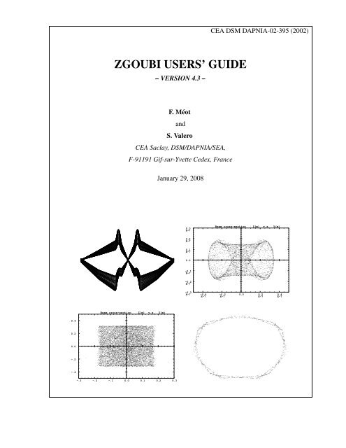
CEA DSM DAPNIA-02-395 (2002)ZGOUBI USERS’ GUIDE– VERSION 4.3 –F. MéotandS. ValeroCEA Saclay, DSM/DAPNIA/SEA,F-91191 Gif-sur-Yvette Cedex, FranceJanuary 29, 20080.3E-7Beam cross-sectionZ(m) v.s. Y(m)0.2E-70.1E-70.0-0.1E-7-0.2E-7-0.3E-7-0.4E-7-0.2E-70.0 0.2E-70.4E-7Beam cross-sectionZ(m) v.s. Y(m)0.40.20.0-.2-.4-.3 -.2 -.1 0.0 0.1 0.2 0.3

0 Cover figures :upper left : colliding proton beams in LHC interaction regions,upper right : sub-micronic non-monochromatic beam cross-section at the imageplane of a second order achromatic micro-beam line,lower left : uniform rectangular beam cross section at the downstream end of a nonlinearbeam expander,lower right : a tracking of defect limited dynamic aperture in LHC.

Table of contentsPART A Description of software contents 5GLOSSARY OF KEYWORDS 7OPTICAL ELEMENTS VERSUS KEYWORDS 9INTRODUCTION 11¡1 NUMERICAL CALCULATION OF MOTION AND FIELDS 131.1 zgoubi Frame . . . . . . . . . . . . . . . . . . . . . . . . . . . . . . . . . . . . . . . . . . . . . . . . . 131.2 Integration of the Lorentz Equation . . . . . . . . . . . . . . . . . . . . . . . . . . . . . . . . . . . . . . 131.2.1 Integration in magnetic fields . . . . . . . . . . . . . . . . . . . . . . . . . . . . . . . . . . . . . 151.2.2 Integration in electric fields . . . . . . . . . . . . . . . . . . . . . . . . . . . . . . . . . . . . . 151.2.3 Integration in combined electric and magnetic fields . . . . . . . . . . . . . . . . . . . . . . . . 171.2.4 Calculation of the time of flight . . . . . . . . . . . . . . . . . . . . . . . . . . . . . . . . . . . 181.3 Calculation of and its Derivatives . . . . . . . . . . . . . . . . . . . . . . . . . . . . . . . . . . . . . 181.3.1 Extrapolation from 1-D axial field map . . . . . . . . . . . . . . . . . . . . . . . . . . . . . . . 181.3.2 Extrapolation from Median Plane Fields . . . . . . . . . . . . . . . . . . . . . . . . . . . . . . . 181.3.3 Extrapolation from arbitrary 2-D Field Maps . . . . . . . . . . . . . . . . . . . . . . . . . . . . 191.3.4 Interpolation in 3-D Field Maps . . . . . . . . . . . . . . . . . . . . . . . . . . . . . . . . . . . 191.3.5 2-D Analytical Field Models and Extrapolation . . . . . . . . . . . . . . . . . . . . . . . . . . . 191.3.6 3-D Analytical Models of Fields . . . . . . . . . . . . . . . . . . . . . . . . . . . . . . . . . . . 191.4 Calculation of from Field Maps . . . . . . . . . . . . . . . . . . . . . . . . . . . . . . . . . . . . . . 201.4.1 1-D Axial Map, with Cylindrical Symmetry . . . . . . . . . . . . . . . . . . . . . . . . . . . . . 201.4.2 2-D Median Plane Map, with Median Plane Antisymmetry . . . . . . . . . . . . . . . . . . . . . 211.4.3 Arbitrary 2-D Map, no Symmetry . . . . . . . . . . . . . . . . . . . . . . . . . . . . . . . . . . 231.4.4 Calculation of from 3-D Field Map . . . . . . . . . . . . . . . . . . . . . . . . . . . . . . . . 241.5 Calculation of and its derivatives . . . . . . . . . . . . . . . . . . . . . . . . . . . . . . . . . . . . . . 251.5.1 Extrapolation from 1-D axial field map . . . . . . . . . . . . . . . . . . . . . . . . . . . . . . . 251.5.2 1-D (Axial) Analytical E-Field Models and Extrapolation . . . . . . . . . . . . . . . . . . . . . . 261.5.3 2-D Analytical E-Field Models and Extrapolation . . . . . . . . . . . . . . . . . . . . . . . . . . 261.5.4 3-D Analytical models of fields . . . . . . . . . . . . . . . . . . . . . . . . . . . . . . . . . . . 261.6 Calculation Of From Field Maps . . . . . . . . . . . . . . . . . . . . . . . . . . . . . . . . . . . . . . 262 SPIN TRACKING 273 SYNCHROTRON RADIATION 293.1 Energy loss and related dynamical effects [10] . . . . . . . . . . . . . . . . . . . . . . . . . . . . . . . . 293.2 Spectral-angular radiated densities [11] . . . . . . . . . . . . . . . . . . . . . . . . . . . . . . . . . . . 303.2.1 Calculation of the radiated electric field . . . . . . . . . . . . . . . . . . . . . . . . . . . . . . . 303.2.2 Calculation of the Fourier transform of the electric field . . . . . . . . . . . . . . . . . . . . . . 324 DESCRIPTION OF THE AVAILABLE PROCEDURES 354.1 Introduction . . . . . . . . . . . . . . . . . . . . . . . . . . . . . . . . . . . . . . . . . . . . . . . . . . 354.2 Definition of an Object . . . . . . . . . . . . . . . . . . . . . . . . . . . . . . . . . . . . . . . . . . . . 354.3 Declaration of options . . . . . . . . . . . . . . . . . . . . . . . . . . . . . . . . . . . . . . . . . . . . . 434.4 Optical Elements and related numerical procedures . . . . . . . . . . . . . . . . . . . . . . . . . . . . . 644.5 Output Procedures . . . . . . . . . . . . . . . . . . . . . . . . . . . . . . . . . . . . . . . . . . . . . . 1224.6 Complementary Features . . . . . . . . . . . . . . . . . . . . . . . . . . . . . . . . . . . . . . . . . . . 1324.6.1 Backward Ray-tracing . . . . . . . . . . . . . . . . . . . . . . . . . . . . . . . . . . . . . . . . 1324.6.2 Checking Fields and Trajectories inside Optical Elements . . . . . . . . . . . . . . . . . . . . . 1324.6.3 Labeling keywords . . . . . . . . . . . . . . . . . . . . . . . . . . . . . . . . . . . . . . . . . . 1333

4.6.4 Multiturn tracking in circular machines . . . . . . . . . . . . . . . . . . . . . . . . . . . . . . . 1334.6.5 Positioning, (mis-)alignement, of optical elements and field maps . . . . . . . . . . . . . . . . . 1334.6.6 Coded integration step . . . . . . . . . . . . . . . . . . . . . . . . . . . . . . . . . . . . . . . . 1354.6.7 Ray-tracing of an arbitrarily large number of particles . . . . . . . . . . . . . . . . . . . . . . . 1354.6.8 Stopped particles: the IEX flag . . . . . . . . . . . . . . . . . . . . . . . . . . . . . . . . . . . . 1354.6.9 Negative rigidity . . . . . . . . . . . . . . . . . . . . . . . . . . . . . . . . . . . . . . . . . . . 135PART B Keywords and input data formatting 137GLOSSARY OF KEYWORDS 139OPTICAL ELEMENTS VERSUS KEYWORDS 141INTRODUCTION 143PART C Examples of input data files and output result files 229INTRODUCTION 2311 MONTE CARLO IMAGES IN SPES 2 2332 TRANSFER MATRICES ALONG A TWO-STAGE SEPARATION KAON BEAM LINE 2363 IN-FLIGHT DECAY IN SPES 3 2394 USE OF THE FITTING PROCEDURE 2425 MULTITURN SPIN TRACKING IN SATURNE 3 GeV SYNCHROTRON 2446 MICRO-BEAM FOCUSING WITH ELECTROMAGNETIC QUADRUPOLES 246PART D Running zgoubi and its post-processor/graphic interface zpop 251INTRODUCTION 2531 GETTING TO RUN zgoubi AND zpop 2531.1 Making the executable files zgoubi and zpop . . . . . . . . . . . . . . . . . . . . . . . . . . . . . . . . . 2531.1.1 The transportable package zgoubi . . . . . . . . . . . . . . . . . . . . . . . . . . . . . . . . . . 2531.1.2 The post-processor and graphic interface package zpop . . . . . . . . . . . . . . . . . . . . . . . 2531.2 Running zgoubi . . . . . . . . . . . . . . . . . . . . . . . . . . . . . . . . . . . . . . . . . . . . . . . . 2531.3 Running zpop . . . . . . . . . . . . . . . . . . . . . . . . . . . . . . . . . . . . . . . . . . . . . . . . . 2532 STORAGE FILES 253REFERENCES 255INDEX 2574

PART ADescription of software contents

7Glossary of keywords£¤¦¥££§©¨§ÄIMANT Generation of a dipole magnet mid-plane 2-D map . . . . . . . . . . . . . . . . . . . . . . . . . . . . . . . . . . . 64AUTOREF Automatic transformation to a new reference frame . . . . . . . . . . . . . . . . . . . . . . . . . . . . . . . . . . 69BEND Bending magnet . . . . . . . . . . . . . . . . . . . . . . . . . . . . . . . . . . . . . . . . . . . . . . . . . . . . . . . . . . . . . . . . . . 70BINARY BINARY/FORMATTED data converter . . . . . . . . . . . . . . . . . . . . . . . . . . . . . . . . . . . . . . . . . . . . 44BREVOL 1-D uniform mesh magnetic field map . . . . . . . . . . . . . . . . . . . . . . . . . . . . . . . . . . . . . . . . . . . . . . 71CARTEMES 2-D Cartesian uniform mesh magnetic field map . . . . . . . . . . . . . . . . . . . . . . . . . . . . . . . . . . . . . 72CAVITE Accelerating cavity . . . . . . . . . . . . . . . . . . . . . . . . . . . . . . . . . . . . . . . . . . . . . . . . . . . . . . . . . . . . . . . 74CHAMBR Long transverse aperture limitation . . . . . . . . . . . . . . . . . . . . . . . . . . . . . . . . . . . . . . . . . . . . . . . . . 76CHANGREF Transformation to a new reference frame . . . . . . . . . . . . . . . . . . . . . . . . . . . . . . . . . . . . . . . . . . . .77CIBLE Generate a secondary beam from target interaction . . . . . . . . . . . . . . . . . . . . . . . . . . . . . . . . . . . 78COLLIMA Collimator . . . . . . . . . . . . . . . . . . . . . . . . . . . . . . . . . . . . . . . . . . . . . . . . . . . . . . . . . . . . . . . . . . . . . . . 79DECAPOLE Decapole magnet . . . . . . . . . . . . . . . . . . . . . . . . . . . . . . . . . . . . . . . . . . . . . . . . . . . . . . . . . . . . . . . . . 80DIPOLE Dipole magnet . . . . . . . . . . . . . . . . . . . . . . . . . . . . . . . . . . . . . . . . . . . . . . . . . . . . . . . . . . . . . . . . . . . 81DIPOLE-M Generation of a dipole magnet mid-plane 2-D map . . . . . . . . . . . . . . . . . . . . . . . . . . . . . . . . . . . 83DIPOLES Dipole magnet -uplet . . . . . . . . . . . . . . . . . . . . . . . . . . . . . . . . . . . . . . . . . . . . . . . . . . . . . . . . . . . 85DODECAPO Dodecapole magnet . . . . . . . . . . . . . . . . . . . . . . . . . . . . . . . . . . . . . . . . . . . . . . . . . . . . . . . . . . . . . . .88DRIFT Field free drift space . . . . . . . . . . . . . . . . . . . . . . . . . . . . . . . . . . . . . . . . . . . . . . . . . . . . . . . . . . . . . . 89EBMULT Electro-magnetic multipole . . . . . . . . . . . . . . . . . . . . . . . . . . . . . . . . . . . . . . . . . . . . . . . . . . . . . . . . 90EL2TUB Two-tube electrostatic lens . . . . . . . . . . . . . . . . . . . . . . . . . . . . . . . . . . . . . . . . . . . . . . . . . . . . . . . . 91ELMIR Electrostatic N-electrode mirror/lens, straight slits . . . . . . . . . . . . . . . . . . . . . . . . . . . . . . . . . . . 92ELMIRC Electrostatic N-electrode mirror/lens, circular slits . . . . . . . . . . . . . . . . . . . . . . . . . . . . . . . . . . . 93ELMULT Electric multipole . . . . . . . . . . . . . . . . . . . . . . . . . . . . . . . . . . . . . . . . . . . . . . . . . . . . . . . . . . . . . . . . 94ELREVOL 1-D uniform mesh electric field map . . . . . . . . . . . . . . . . . . . . . . . . . . . . . . . . . . . . . . . . . . . . . . . .96END End of input data list ; see FIN . . . . . . . . . . . . . . . . . . . . . . . . . . . . . . . . . . . . . . . . . . . . . . . . . . . . . 45ESL Field free drift space . . . . . . . . . . . . . . . . . . . . . . . . . . . . . . . . . . . . . . . . . . . . . . . . . . . . . . . . . . . . . . 89FAISCEAU Print particle coordinates . . . . . . . . . . . . . . . . . . . . . . . . . . . . . . . . . . . . . . . . . . . . . . . . . . . . . . . . . 123FAISCNL Store particle coordinates in file FNAME . . . . . . . . . . . . . . . . . . . . . . . . . . . . . . . . . . . . . . . . . . 123FAISTORE Store coordinates every other pass at labeled elements . . . . . . . . . . . . . . . . . . . . . . . . . . . 123FFAG FFAG magnet, -uplet . . . . . . . . . . . . . . . . . . . . . . . . . . . . . . . . . . . . . . . . . . . . . . . . . . . . . . . . . . . 97FFAG-SPI Spiral FFAG magnet, -uplet . . . . . . . . . . . . . . . . . . . . . . . . . . . . . . . . . . . . . . . . . . . . . . . . . . . . . 99FIN End of input data list . . . . . . . . . . . . . . . . . . . . . . . . . . . . . . . . . . . . . . . . . . . . . . . . . . . . . . . . . . . . . . 45FIT Fitting procedure . . . . . . . . . . . . . . . . . . . . . . . . . . . . . . . . . . . . . . . . . . . . . . . . . . . . . . . . . . . . . . . . . 46FOCALE Particle coordinates and horizontal beam dimension at distance . . . . . . . . . . . . . . . . . . 124FOCALEZ Particle coordinates and vertical beam dimension at distance . . . . . . . . . . . . . . . . . . . . .124GASCAT Gas scattering . . . . . . . . . . . . . . . . . . . . . . . . . . . . . . . . . . . . . . . . . . . . . . . . . . . . . . . . . . . . . . . . . . . . 51HISTO 1-D histogram . . . . . . . . . . . . . . . . . . . . . . . . . . . . . . . . . . . . . . . . . . . . . . . . . . . . . . . . . . . . . . . . . . 125IMAGE Localization and size of horizontal waist . . . . . . . . . . . . . . . . . . . . . . . . . . . . . . . . . . . . . . . . . . . 124IMAGES Localization and size of horizontal waists . . . . . . . . . . . . . . . . . . . . . . . . . . . . . . . . . . . . . . . . . . 124IMAGESZ Localization and size of vertical waists . . . . . . . . . . . . . . . . . . . . . . . . . . . . . . . . . . . . . . . . . . . . 124IMAGEZ Localization and size of vertical waist . . . . . . . . . . . . . . . . . . . . . . . . . . . . . . . . . . . . . . . . . . . . . 124MAP2D 2-D Cartesian uniform mesh field map - arbitrary magnetic field . . . . . . . . . . . . . . . . . . . . . 100MAP2D-E 2-D Cartesian uniform mesh field map - arbitrary electric field . . . . . . . . . . . . . . . . . . . . . . . 101MARKER Marker . . . . . . . . . . . . . . . . . . . . . . . . . . . . . . . . . . . . . . . . . . . . . . . . . . . . . . . . . . . . . . . . . . . . . . . . . 102MATPROD Matrix transfer . . . . . . . . . . . . . . . . . . . . . . . . . . . . . . . . . . . . . . . . . . . . . . . . . . . . . . . . . . . . . . . . . . 103MATRIX Calculation of transfer coefficients, periodic parameters . . . . . . . . . . . . . . . . . . . . . . . . . . . . . 126MCDESINT Monte-Carlo simulation of in-flight decay . . . . . . . . . . . . . . . . . . . . . . . . . . . . . . . . . . . . . . . . . . .52MCOBJET Monte-Carlo generation of a 6-D object . . . . . . . . . . . . . . . . . . . . . . . . . . . . . . . . . . . . . . . . . . . . .36MULTIPOL Magnetic multipole . . . . . . . . . . . . . . . . . . . . . . . . . . . . . . . . . . . . . . . . . . . . . . . . . . . . . . . . . . . . . . 104OBJET Generation of an object . . . . . . . . . . . . . . . . . . . . . . . . . . . . . . . . . . . . . . . . . . . . . . . . . . . . . . . . . . . 39OBJETA Object from Monte-Carlo simulation of decay reaction . . . . . . . . . . . . . . . . . . . . . . . . . . . . . . . 42OCTUPOLE Octupole magnet . . . . . . . . . . . . . . . . . . . . . . . . . . . . . . . . . . . . . . . . . . . . . . . . . . . . . . . . . . . . . . . . 105ORDRE Taylor expansions order . . . . . . . . . . . . . . . . . . . . . . . . . . . . . . . . . . . . . . . . . . . . . . . . . . . . . . . . . . . 54

8¤¥ PARTICUL Particle characteristics . . . . . . . . . . . . . . . . . . . . . . . . . . . . . . . . . . . . . . . . . . . . . . . . . . . . . . . . . . . . 55PICKUPS Beam centroid path; closed orbit . . . . . . . . . . . . . . . . . . . . . . . . . . . . . . . . . . . . . . . . . . . . . . . . . . 127PLOTDATA Intermediate output for the PLOTDATA graphic software . . . . . . . . . . . . . . . . . . . . . . . . . . . 128POISSON Read magnetic field data from POISSON output . . . . . . . . . . . . . . . . . . . . . . . . . . . . . . . . . . . 106POLARMES 2-D polar mesh magnetic field map . . . . . . . . . . . . . . . . . . . . . . . . . . . . . . . . . . . . . . . . . . . . . . . 107PS170 Simulation of a round shape dipole magnet . . . . . . . . . . . . . . . . . . . . . . . . . . . . . . . . . . . . . . . . 108QUADISEX Sharp edge magnetic multipoles . . . . . . . . . . . . . . . . . . . . . . . . . . . . . . . . . . . . . . . . . . . . . . . . . . 109QUADRUPO Quadrupole magnet . . . . . . . . . . . . . . . . . . . . . . . . . . . . . . . . . . . . . . . . . . . . . . . . . . . . . . . . . . . . . .110REBELOTE Jump to the beginning of zgoubi input data file . . . . . . . . . . . . . . . . . . . . . . . . . . . . . . . . . . . . . . 56RESET Reset counters and flags . . . . . . . . . . . . . . . . . . . . . . . . . . . . . . . . . . . . . . . . . . . . . . . . . . . . . . . . . . . 57SCALING Time scaling of power supplies and R.F. . . . . . . . . . . . . . . . . . . . . . . . . . . . . . . . . . . . . . . . . . . . . 58SEPARA Wien Filter - analytical simulation . . . . . . . . . . . . . . . . . . . . . . . . . . . . . . . . . . . . . . . . . . . . . . . . 112SEXQUAD Sharp edge magnetic multipole . . . . . . . . . . . . . . . . . . . . . . . . . . . . . . . . . . . . . . . . . . . . . . . . . . . 109SEXTUPOL Sextupole magnet . . . . . . . . . . . . . . . . . . . . . . . . . . . . . . . . . . . . . . . . . . . . . . . . . . . . . . . . . . . . . . . 113SOLENOID Solenoid . . . . . . . . . . . . . . . . . . . . . . . . . . . . . . . . . . . . . . . . . . . . . . . . . . . . . . . . . . . . . . . . . . . . . . . .114SPNPRNL Store spin coordinates into file FNAME . . . . . . . . . . . . . . . . . . . . . . . . . . . . . . . . . . . . . . . . . . . 129SPNPRNLA Store spin coordinates every other pass . . . . . . . . . . . . . . . . . . . . . . . . . . . . . . . . . . . . . . . . .129SPNPRT Print spin coordinates . . . . . . . . . . . . . . . . . . . . . . . . . . . . . . . . . . . . . . . . . . . . . . . . . . . . . . . . . . . . 129SPNTRK Spin tracking . . . . . . . . . . . . . . . . . . . . . . . . . . . . . . . . . . . . . . . . . . . . . . . . . . . . . . . . . . . . . . . . . . . . .60SRLOSS Synchrotron radiation loss . . . . . . . . . . . . . . . . . . . . . . . . . . . . . . . . . . . . . . . . . . . . . . . . . . . . . . . . . 62SRPRNT Print SR loss statistics . . . . . . . . . . . . . . . . . . . . . . . . . . . . . . . . . . . . . . . . . . . . . . . . . . . . . . . . . . . 130SYNRAD Synchrotron radiation spectral-angular densities . . . . . . . . . . . . . . . . . . . . . . . . . . . . . . . . . . . . . 63TARGET Generate a secondary beam from target interaction ; see CIBLE . . . . . . . . . . . . . . . . . . . . . . . 78TOSCA 2-D and 3-D Cartesian or cylindrical mesh field map . . . . . . . . . . . . . . . . . . . . . . . . . . . . . . . . 115TRAROT Translation-Rotation of the reference frame . . . . . . . . . . . . . . . . . . . . . . . . . . . . . . . . . . . . . . . . 116TWISS Calculation of optical parameters ; periodic parameters . . . . . . . . . . . . . . . . . . . . . . . . . . . . . .131UNDULATOR Undulator magnet . . . . . . . . . . . . . . . . . . . . . . . . . . . . . . . . . . . . . . . . . . . . . . . . . . . . . . . . . . . . . . . 117UNIPOT Unipotential cylindrical electrostatic lens . . . . . . . . . . . . . . . . . . . . . . . . . . . . . . . . . . . . . . . . . . 118VENUS Simulation of a rectangular dipole magnet . . . . . . . . . . . . . . . . . . . . . . . . . . . . . . . . . . . . . . . . . 119WIENFILT Wien filter . . . . . . . . . . . . . . . . . . . . . . . . . . . . . . . . . . . . . . . . . . . . . . . . . . . . . . . . . . . . . . . . . . . . . . 120YMY Reverse signs of and reference axes . . . . . . . . . . . . . . . . . . . . . . . . . . . . . . . . . . . . . . . . . . .121

9Optical elements versus keywordsThis glossary gives a list of keywords suitable for the simulation of common optical elements. These are classifiedin three categories: magnetic, electric and electromagnetic elements.Field map procedures are also cataloged; they provide a mean for ray-tracing through measured fields, or as wellthrough field maps obtained from numerical simulations of arbitrary geometries with such tools as POISSON, TOSCA,etc.MAGNETIC ELEMENTSDecapoleDipoleDodecapoleFFAG magnetsMultipoleOctupoleQuadrupoleSextupoleSkewed multipolesSolenoidUndulatorDECAPOLE, MULTIPOLAIMANT, BEND, DIPOLE, DIPOLE-M, MULTIPOL, QUADISEXDODECAPO, MULTIPOLDIPOLES, FFAG, FFAG-SPI, MULTIPOLMULTIPOL, QUADISEX, SEXQUADOCTUPOLE, MULTIPOL, QUADISEX, SEXQUADQUADRUPO, MULTIPOL, SEXQUADSEXTUPOL, MULTIPOL, QUADISEX, SEXQUADMULTIPOLSOLENOIDUNDULATORField maps1-D, cylindrical symmetry2-D, mid-plane symmetry2-D, no symmetry2-D, polar mesh, mid-plane symmetry3-D, no symmetryBREVOLCARTEMES, POISSON, TOSCAMAP2DPOLARMESTOSCAELECTRIC ELEMENTS2-tube (bipotential) lens3-tube (unipotential) lensDecapoleDipoleDodecapoleMultipoleN-electrode mirror/lens, straight slitsN-electrode mirror/lens, circular slitsOctupoleQuadrupoleR.F. (kick) cavitySextupoleSkewed multipolesEL2TUBUNIPOTELMULTELMULTELMULTELMULTELMIRELMIRCELMULTELMULTCAVITEELMULTELMULTField maps1D, cylindrical symmetry ELREVOL2-D, no symmetryMAP2D

10ELECTROMAGNETIC ELEMENTSDecapoleDipoleDodecapoleMultipoleOctupoleQuadrupoleSextupoleSkewed multipolesWien filterEBMULTEBMULTEBMULTEBMULTEBMULTEBMULTEBMULTEBMULTSEPARA, WIENFILT

11INTRODUCTIONThe computer code zgoubi calculates trajectories of charged particles in magnetic and electric fields. At the originspecially adapted to the definition and adjustment of beam lines and magnetic spectrometers, it has so evolved that itallows the study of systems including complex sequences of optical elements such as dipoles, quadrupoles, arbitrarymultipoles, FFAG magnets and other magnetic or electric devices, and is able as well to handle periodic structures.Compared to other codes, it presents several peculiarities:a numerical method for integrating the Lorentz equation, based on Taylor series, which optimizes computing timeand provides high accuracy and strong symplecticity,spin tracking, using the same numerical method as for the Lorentz equation,calculation of the synchrotron radiation electric field and spectra in arbitrary magnetic fields, from the ray-tracingoutcomes,the possibility of using a mesh, which allows ray-tracing from simulated or measured (1-D, 2-D or 3-D) field maps,numerous Monte Carlo procedures: unlimited number of trajectories, in-flight decay, photon emission, etc.a built-in fitting procedure including arbitrary variables and a large variety of constraints,multiturn tracking in circular accelerators including features proper to machine parameter calculation and survey,simulation of time-varying power supplies.The initial version of the Code, dedicated to ray-tracing in magnetic fields, was developed by D. Garreta and J.C. Faivreat CEN-Saclay in the early 1970’s. It was perfected for the purpose of studying the four spectrometers SPES I, II, III, IVat the Laboratoire National Saturne (CEA-Saclay, France), and SPEG at Ganil (Caen, France). It is being used since longin several national and foreign laboratories.The first manual was in French [1]. Since then many improvements have been implemented. In order to facilitate accessto the program an English version of the manual was written at TRIUMF with the assistance of J. Doornbos. P. Stewartprepared the manuscript for publication [2]An updating was necessary for accompanying the third version of the code which featured spin tracking and ray-tracingin combined electric and magnetic fields; this was done with the help of D. Bunel for the preparation of the document andlead to the third release [3].Lately, provisions were introduced for the computation of synchrotron radiation electromagnetic impulse and spectra.In the mean time, several new optical elements were added, such as electro-magnetic and other electrostatic lenses. Usedsince several years for special studies in periodic machines (e.g., SATURNE at Saclay, COSY at Julich, LEP and LHC atCern), zgoubi has also benefited from extensive development of storage ring related features.These developments of zgoubi have strongly benefited of the environment of the Groupe Théorie, Laboratoire NationalSATURNE, CEA/DSM-Saclay.The graphic interface to zgoubi (addressed in Part D) has also undergone concomitent extended developments, whichmake it a performant tool for post-processing zgoubi outputs.This manual is intended only to describe the details of the most recent version of zgoubi , which is far from being a“finished product”.

!!%" && 131 NUMERICAL CALCULATION OF MOTION AND FIELDS1.1 zgoubi FrameThe reference frame of zgoubi is presented in Fig 1. Its origin is in the median plane on a reference curve which coincideswith the optical axis of optical elements.1.2 Integration of the Lorentz EquationThe Lorentz equation, which governs the motion of a particle of charge , relativistic massand magnetic fields and , is written and velocity in electric (1.2.1) ←VTrajectoryZMPY0←WReferenceXTFigure 1: Reference frame and coordinates ( , , , ¥ ) in zgoubi .!§ : in the plane of the reference curve in the direction of motion, ! § §#"$ §#"$ § ¥ : in the plane of the reference curve, normal to ,: orthogonal to the plane,: projection of the velocity, , in the plane,= angle between and the -axis,= angle between and .Taking¡-,& ('where ¡-, is the rigidity of the particle, this equation can be rewritten" &*) (' "+ &(1.2.2)

14 1 NUMERICAL CALCULATION OF MOTION AND FIELDSThe derivatives &WVEXZY &X&' ¡., & ¡-, [VDXZY ¡-, & :X'¡., X : :'' ¡-, ) :'?>@''?>CBDBEB? @A> 'KBDBDBL @JA ¡., ) ) ) )'QTUJA'?FGHA'?MNA ¡., /)(1.2.3)&0 ¡.,&*) &#From position 1 3254following a displacement :, position 1 3287, are obtained from truncated Taylor expansions (Fig. 2)297and unit velocity & 3254at pointat point264and unit velocity & 3287& ) ) ) ) ) :(1.2.4)1 ;2 7= ('TT ¦'P P ('P 'A (1.2.6)R3297S

1.2 Integration of the Lorentz Equation 15The successive derivatives &WVEXZY where ¡ VEXZY ¡¡X¡¡b^X¡^&¡ ¡^¡ >bT ¡b g ^bP ¡g ^^¡ >bj¡ )¦b¡b^¡§¡) ) ¡) )¦ ¡b^¡ >b^¡ >b) ) ) ¡) ) ) ¡T ¡b g ^bb^¡^¡1.2.1 Integration in magnetic fieldsAdmitting that K\ " and noting ¡, eq. (1.2.3) reduces to¡.,&*) &#('X of & needed in the Taylor expansions (eqs. 1.2.4) are calculated by differentiating&#& ) & ) &#¡ )(1.2.7)& ) ) &*)O&#&*) ) ) &I) )-¡ @&I)O&#&I) ) ) ) &I) ) )O¡ U&*) )]¡ )( U& ) &#¡ ) ) ) )& ) ) ) ) ) & ) ) ) ) ¡ R& ) ) ) ¡ ) G& ) ) ¡ ) ) RX .From, and by successive differentiation, we get('¡ _^§ ^ a`CbDc 7ed T ^^ ^ §^ §^ ¡ ) fb & b^ §g & b & g f¡ ) ) fb &I) bbhg^ §(1.2.8)^ §^ §) ) ) f ¡bigkjg & )b & g fj & b & g & j U fb & ) ) b^ §^ §^ §big^ §^ §^ §j &m)b & g & j) ) ) ) f ¡bigkj[ll & b & g & j & l G f^ §^ §^ §^ §^ §bhgkj^ §^ §g & )b & ) g f R fbig& ) ) b & g U fbig gb & ) ) ) b^ §;254From the knowledge 3254 ofand ¡ &of the trajectory, we calculate alternately the derivatives of & 3294.^ §^ §^ §^ §264at pointand ¡ 3264, by means of eqs. (1.2.7) and (1.2.8), and inject it in eq. (1.2.4) to get 1 3287and & 32871.2.2 Integration in electric fields [4]Admitting that K\ " eq. (1.2.3) reduces to&0 ¡.,& ) ¡., )(1.2.9)which, by successive differentiations, gives the recursive relations

16 1 NUMERICAL CALCULATION OF MOTION AND FIELDS€ XX ¡., ) ¡., ) ) ¡., ) ) ) ))X&¡., ) & ¡-,¡., ) & ) ) ) w G¡.,¡., ) & ) ) ) ) w¡.,b^)\q¡., ) ) & ) ) w{R¡-,¢^¡., ) ) & ) ) ) w¡.,¢ >bT ¢b g ^¡., ) & ) w¡.,¢)))) ¡-, ) ) & ¡-,¡-, ) ) ) & ) w¡.,q\b¡., ) & ) ) w U¡-,¡., ) ) ) ) & ¡.,¡-, ) ) ) & ) ) w N¡-,^¢¢€^¡., ) ) & ) w¡.,¡-, ) ) ) ) & ) w¡.,¢ >b^¢€€))¡., ) ) ) & ¡.,¡., ) ) ) ) ) & ¡.,Xb^¢¢ ) ) ) ) x yZz&n ¡.,& ) ¡., ) ) )) ) porqts&(1.2.10)&0 @ ¡., )I& ) ¡.,) )U ¡-, ) ) & ) U ¡., )&n& ) ) ) uorqI @ o*q ) ) )& ) ) ¡.,ovq.s.sWsR ¡-, ) ) ) & ) G ¡., ) ) & ) ) R ¡., )&n& ) ) ) ) & ) ) ) ¡-,) ) )) )q o.sU o qWs) U o qWsq ) ) ) ) )that provide the derivativesX needed in the Taylor expansions (eq. 1.2.4)('¢awuorq s&*)¢ ).x yZz w @ o q ¢Ws& ) ) q oWs).x yZz q ¢) )& ) ) ) q oWs @ o q ¢ts(1.2.11)¢ ) ).x yZz w U¢ ) ) x yZz o*q¢ ) ) ) x yz) ) )&*) ) ) ) orqWs¢ U o*q) )¢ ) x yZz U o*q.sWstswR¢ ) ) ) x yz| o*q) ) ) )) ) ) ) ) uorqWs&¢ R o*q) ) )¢ ) x yZz| G o*q) )¢ ) ) x yZz} R o*q.sWsWsWsw Nwhere ¢field are obtained from the total derivativeeVEXZY x yZzdenotes differentiation at constant ¡., : ¢ VEXZY x yz , and ¡.,¡-, q('X . These derivatives of the electricby successive differentiations¢ p^§ ^ ^ ^ ^ § (1.2.12)¢ ) fb & b^ §(1.2.13)¢ ) ) fb &~)bbhgg & b & g f^ §^ §^ §) ) ) f ¢bigkjj & b & g & j U fb & ) ) bg & )b & g fbigetc. as in eq. 1.2.8. These eqs. (1.2.11), as well as the calculation of the rigidity, following eq. (1.2.5), involve derivatives ¡., eVEXZY ¡., , which are obtained in the following way. Considering that^ §^ §^ §^ §^ §^ §('Q€>€~>i.e.,€ (1.2.14)with (eq. 1.2.1), we obtain

1.2 Integration of the Lorentz Equation 17€ ¡., ) ¡., ) ) ¡., ) ) ) )€ ¡-, ) ¡-, ) _orq sˆ) ¡-, ˆ) ) ) ¡-, ) ) ) ) X&)XX %w€Š> 4)€7% X 7 ¡., ) ¡-,))€¡., ) ¡.,¡-, ) ¡.,w€¡-, ) ) ¡-,)€)¡., ) ) ¡-,w¡-, ) ) ) ¡.,ŠŠ> 4 %4€ Wƒ(1.2.15)I5‚ „ƒ‚ …ƒ †\since. Normalizing as previously witheq. (1.2.15) leads to the ¡., ‡VEXZY& ¡-,&and¦' , and by successive differentiations,qvƒ&m) rƒ(1.2.16)q&m/)rƒ&~-) ) ) qvƒq ots&]ˆ) )rƒ@ o qWs&~-rƒ&m/)¦q) ) ) orqts) ) ) „ƒvƒU orqWs&]O&]ˆ) ) )„ƒU orqWs&]ˆ)(vƒ&~/) )¦Note that the derivatives&mcan be related to the derivatives of the kinetic energy by% X('nƒ&meVEXY which leads tovƒ rƒ ƒrƒX‰&mX (1.2.17)¦'('X‰Finally, the derivatives .sovqVDXZYovq sX('€involved in eqs. (1.2.11,1.2.16) are obtained fromŠ % , (isthe rest mass) by successive differentiations, that give the recursive relationsŠ> ‹qovq.s¡-,&]orqs q(1.2.18)Š> ‹qvƒ¡.,) )Š> ‹qq oWsvƒ&] )¡-,@ o q wWsqo*qWs) ) )Š> qvƒ&] ) )¡-,U o*q wWs) )qU o*q w.s1.2.3 Integration in combined electric and magnetic fieldsWhen both and are non-zero, the complete eq. (1.2.3) must be considered. Recursive differentiations give the followingrelations&n ¡-,& ) &#&n @ ¡., )I ) &© ¡., ) ) )(1.2.19)& ) ¡., )) ) porqts&ovq.s) )U ¡., ) ) & ) U ¡-, )&0& ) ) ) _orqI @ o*q ) ) ) &©& ) ) ¡-, ) )o*qWsWsWsR ¡., ) ) ) & ) G ¡-, ) ) & ) ) R ¡., )&n& ) ) ) ) & ) ) ) ¡-,) ) )) ) ) ) ) ) ) &orqWsU o*qWs) U o*q.sq ) ) )that provide the derivativesX needed in the Taylor expansions (1.2.4)('

18 1 NUMERICAL CALCULATION OF MOTION AND FIELDSwhere ¢))¡., ) & ¡.,¡., ) & ) ) ) w G¡.,¡., ) ) & ) ) w{R¡-,¡., ) & ) w¡.,¡-, ) ) ) & ) w¡.,¡., ) ) & ¡-,, and denotes differentiation at constant ¡-,yZz x VDXZY ¡-,XX¡., ) &*) ) w U¡.,¡-, ) ) ) ) & ¡.,¡-, ) ) &*) w¡-,¡., ) ) ) & ¡.,These derivatives ¢ VDXZYand ¡ VEXZYof the electric and magnetic fields are calculated from the vector fields ¢ ^g b‰bb‰g‰j ¢b g ^j ¡ ‰g>>b‰g‰j ¡b g ^>^ Rq>Tq- :T'PR ^ GPMR ^ U”q¡ Ž MMM&#uorqWs&*)¢ ¡ w) ) uo qWs& o q ¢Ws¢ )-x yZz|&#¡ ) ).x yZz w @) )¢ ) ) x yZz (1.2.20)¡ /) ) x yZz w U) ) uorq s&*) @ orq ¢s ) x yZz q ¢&#¢ ) x yz U ) ) )) )¢ ) ) x yZz o q¢ ) ) ) x yZzq oWs U o q ¢Wsq&*) ) ) ) /)ts¡ ) ) )Wx yz w*R&#, ¡ ¡-,and VDXZY B(1.2.21)&# VEXY x yZz q ¡.,¡&#VEXZY x yZz q ¡.,¢('§#"kS"e ,¡ §©"$Œ"[ and their derivativesj andj , following eqs. (1.2.8) and (1.2.13).1.2.4 Calculation of the time of flight^ §^ ^ § ^ ^ ^The time of flight eq. (1.2.6) involves the r (' derivatives* ¦'?> ,eq. (1.2.18). In the absence of electric field eq. (1.2.7) however reduces to the simple form>~¦', etc. that are obtained from(1.2.22) ;29732541.3 Calculation of ¡ and its Derivatives§©"$Œ"[ and derivatives are calculated in various ways, depending whether field maps or analytic representations of¡optical elements are used. The basic means are the following.1.3.1 Extrapolation from 1-D axial field map [5]A cylindrically symmetric field (e.g., using BREVOL) can be described by an axial 1-D field map of its longitudinalcomponent†\ > 7/‘ , while the radial component on axis ¡|’ §#"/ C\ is assumed to be zero. ¡ Ž §#"$is obtained at any point along the -axis by a polynomial interpolation from the map mesh (see section§#"$¡„Ž “\ § 1.4.1). §#"/ Then the field components §#"/ , at the position of the particle, §#"/ are obtained from Taylor ’ ¡ ¡}Žexpansions truncated at the fifth order insymmetry(hence, up to the fifth order derivative ^> ¡ ŽP ¡ Ž§#" \ ), assuming cylindrical^ § ¡ Ž §#" \ w§#"/\ O §#"¡ Ž T\ §#"¡ Ž M¡ Ž ¡ ’ ¡„Ž(1.3.1)^ §^ §By differentiation with respect § toFinally a conversion from the§§§^ ^ ând , up to the second order, these expressions provide the §#"/ derivatives of .coordinates to ¡ the Cartesian coordinates of zgoubi is performed, thus §#"kS"e §©"/§#"/ w§#" \ w@ ^§#" \ OG ^§#" \ providing the expressionsj needed in the eq. (1.2.8).1.3.2 Extrapolation from Median Plane Fields^ §^ ^ In the median §#"kS" \ plane, , and its derivatives with respect § to ¡}• or , may be calculated from analytical models(e.g. in Venus magnet - VENUS, and sharp edge multipoles SEXQUAD and QUADISEX) or numerically by polynomialinterpolation from 2-D field maps (e.g. CARTEMES, TOSCA).

4Ž ^ ˜ ¡§ ^"– ^ ˜ ¡ ^¡wTGThe scalar potential used for the calculation of ^¡@w>"To ^ G> ¡T ¡¡ T>• ^ ˜ ¡ ^‰g‰j ¡ bb¡ >s>X4b^T ¡T ¡T ^s>Psw^ww>˜P ¡4^¡ P>^>˜4¡ PsPq1.3 Calculation of ¡ and its Derivatives 19Median plane antisymmetry is assumed, which results in¡ Ž ¡ Ž wr¡ Ž (1.3.2)§#"kS" \ †\¡ – §#"kS" \ †\§#"kS"e §#"kS" §#"kS"e wr¡ – §#"kS" ¡|– §#"kS"e ¡ • §#"kS"¡|• Accomodated with Maxwell’s equations, this results in Taylor expansions below, for the three components of (here, ¡stands for ¡|• ¡ \ ) §©"$Œ" T ¡ Ž (1.3.3)§#"kS"e ô ^^ §^ §^ § ^ ¡|– §#"kS"e ^^ ^ §^ ^ ¡|• §#"kS"e ¡—w@ Ro*^> ô*^P @> ^which are then differentiated one by one with respect to § , , or , up to second or fourth order (depending on opticalelement or IORDRE option, see section 1.4.2) so as to get the expressions involved in eq. (1.2.8).^ §^ ^ §^ §^ ^ 1.3.3 Extrapolation from arbitrary 2-D Field Maps2-D field maps that §#"kS"e give the §#"$Œ"[ three components §#"kS"e , and at §©"$ each node of a-elevation map may be used. and its derivatives at any pointŽ ¡|– are calculated by polynomial interpolation¡¡ ¡|• §#"$Œ"[ followed by Taylor expansions in , without any hypothesis of symmetries (see section 1.4.3 and keywords MAP2D,MAP2D-E).1.3.4 Interpolation in 3-D Field Maps [6]In 3-D field maps ¡and its derivatives up to the second order with respect § to , , or are calculated by means of asecond order polynomial interpolation, from 3-D U 3-point grid (see section 1.4.4).U1.3.5 2-D Analytical Field Models and ExtrapolationSeveral optical elements such as BEND, WIENFILT (that uses the BEND procedures), QUADISEX, VENUS, etc., aredefined from the expression of the field and derivatives in the median plane. 3-D extrapolation of these off the median isdrawn from Taylor expansions.1.3.6 3-D Analytical Models of FieldsIn many optical elements such as QUADRUPO, SEXTUPOL, MULTIPOL, EBMULT, etc., the three components of ¡and their derivatives with respect § to , or are obtained at any step along trajectories from analytical expressionfollowing§#"kS"edrawn from the scalar potential ˜¡ Ž¡ Ž" etc. (1.3.4)> " ^" ^^ §Multipoles^ § ^ ^ ^ §electro-magnetic multipoles with poles (namely, QUADRUPO ( ž @to 10), EBMULT ( ž @Ÿž to 10)) is [7] q) to DODECAPO ( ž G), MULTIPOL ( ž j ( 8š›œ \to R ) in the case of magnetic and§#"kS"e ^ §^ ^

20 1 NUMERICAL CALCULATION OF MOTION AND FIELDSsolutions of the normal equations^'·b¥ ž…A 47 ¨ wqq¢ >¢ Y V'« ² > ¨³47bR'« ³¥>§>>> ¢>'« ³§TTT>Xfc 4§©§P''« ³PP§MbM'« ³M>§>©¡ >nf¢ 4 c§ ª©@S« X(¬ § A ® (1.3.5)¢I£ž#¨˜ X§#"$Œ"[ A ž wA ž A ¤p¥¦where§ is the longitudinal gradient, defined at the entrance or exit of the optical element by£ £ 3'£ 4£ 44 ¡X4 (1.3.6)1 3'$ "wherein5¯ °(±3' ² ² ² M ¨ ² T ändis the distance to the EFB. ² P ¨Skewed multipolesž ´ X§ §#"kOµI"[…µ §©"$]µI"[…µ §#"$Œ"[ §#"$mµI"[=µ §©"$Œ"[ §©"$mµ"e…µ ´ XA multipole component with arbitrary order can be tilted independently of the others by an arbitrary angle aroundthe -axis. If so, the calculation of the field and derivatives in the rotated axisis done in two steps. First,they are calculated at the rotated position, in the frame, as derived from expression (1.3.5) above.Second, and its derivatives atin the frame are transformed to the rotatedframe bya rotation of the same angle .In particular a skewed @Ÿž -pole component is created by taking ´ X .@Zž¡ 1.4 Calculation of from Field Maps1.4.1 1-D Axial Map, with Cylindrical SymmetryLet bethe value of the longitudinal §#"/ †\ component of the field , at node of a uniform mesh that definesa 1-D field map along the symmetry ¡ -axis, while ¡}’ 7/‘ b ¡}Ž >¡is assumed to be zero . The field§ §#"/ \ u\ component is calculated by a polynomial interpolation of the fifth degree § in , using a 5 points §#"/ gridŽ ¡centered at the node of the 1-D map which is closest to the actual § coordinateThe interpolation polynomial isof the particle.¡ ´ ´ ´ ´(1.4.1)§#" \ ´§ ánd the coefficients áre calculated by expressions that minimize the quadratic sum· f ¡ (1.4.2)§#" \ w6¡ b Namely, the source code contains the explicit analytical expressions of the ´bcoefficients.C\´X ¡ ^The§ X §#" \ derivatives at the actual § position , as involved in eqs. (1.3.1), are then obtained by differentiation ofthe polynomial (1.4.1), giving^ ^

in fourth order. The coefficients ´The ´^·^^^¡ >¡ MM¡>´ ´ §§qTP´7´ ´ M´´>§§T>T´q@§T´7 §>§P>>§>>>´§P @ \ ´´ >´ T§MT 47 Tare calculated by expressions that minimize, with respect to ´· fmay then be identified with the derivatives of ¡ ^^¡¡´q^‰bb ´g´§>>´4 >TT´T§M4 > ´P4 >>4 P>1.4 Calculation of ¡ from Field Maps 21 @ R N§#" \ ´§ U§#" \ @(1.4.3)^ §> G§ ^ §B B B1.4.2 2-D Median Plane Map, with Median Plane AntisymmetryLet be the value of ¡|• §©"$Œ" \ at the nodes of a mesh which defines a 2-D field map in the (§#"$ plane while¡ Ž ¡ \ bhg and ¡|– §#"kS" \ are assumed to be zero. Such a map may have been built or measured in either Cartesian§#"kS" or polar coordinates. Whenever polar coordinates are used, a change to Cartesian coordinates (described below) providesthe expression of and its derivatives as involved in eq. (1.2.8).zgoubi provides three types of polynomial interpolation from the mesh (option IORDRE); namely, a second order interpolation,with either a 9- or a 25-point grid, or a fourth order interpolation with a 25-point grid (Fig. ¡ 3).If the 2-D field map is built up from simulation, the grid simply aims at interpolating the field at a given point from its 9or 25 neighbors. If the map results from measurements, the grid also smoothes field measurement fluctuations.The mesh may be defined in Cartesian coordinates, (Figs. 3A and 3B) or in polar coordinates (Fig. 3C).The interpolation grid is centered on the node which is closest to the projection (§#"k in the plane of the actual point ofthe trajectory.The interpolation polynomial is§#" \ @ \ ´^ §in second order, or§©"$Œ" \ ´¡ ´§ ´ ´> 4 ´§© ´(1.4.4)4k47ˆ44‡77k77$7¡ 4k4§#"kS" \ ´7ˆ44‡7§ ´ ´> 4´ 4 T> 7 ´P(1.4.5)§© ´ ´§©, the quadratic sumP 4T 7 ´>$>§©big(1.4.6)bhg ¡ §©"$Œ" \ w6¡ bhg The source code contains the explicit analytical expressions of the ´bigcoefficients.†\solutions of the normal equationsbhgbig^ ´bhg§©"$Œ" \ at the central node of the gridg ¡\ " \ " \ (1.4.7)bhg and , at the actual pointinterpolation polynomial, which gives (e.g. from (1.4.4) in the case of second order interpolation)The derivatives §#"$Œ" \ of with respect § to ¡^ §^ §#"kS" \ are obtained by differentiation of theA š A7¸47$7^ §(1.4.8)§ ´§#"$Œ" \ ´ @> 47k7^ etc.4e7§#"$Œ" \ ´§ @This allows stepping to the calculation §#"kS"e of and its derivatives as described in subsection 1.3.2 (eq. 1.3.3).¡The special case of polar mapsIt is necessary to change from polar map frame ( 1 "$¹Œ"[ ) to the Cartesian moving frame (§#"$Œ"[ ). This is done as follows.

22 1 NUMERICAL CALCULATION OF MOTION AND FIELDSIn second order calculations the correspondence is (we note • C\ )¡“º†¡^§¡^^> ¡ ^^§ ^¡»^ 1^1 ^ q¹ ¡ ^ 1 > ^ > > q q 1 ^^> ¡ > ¡ ¹ ^^§ ^ > ¡ ^¡> ¡1 q ^ 1^ > ¡ ¹ ^^ > 1 > »^T ¡ U ^ ^^§ ^^§ ^T¡ T> T ¡ ^^§ ^ T ¡ ^^ ^T> ¡ >1> ^ 1¹ ^ w @ > ¡ ^ww¡11 > ^ q¹ ^@T ^ 1T 1 > ^ w q 1 > ^^ @ ¡ @ > ¡ ¹ ^T ^ 1¹ ^C\w> 1 ^ 1^ ¹ ^¡¡¹ ^ ¡ ¡ >1 ^ 1 > q 1In fourth order calculations the relations are the same up to second order, and thenT T ¡¡T q 1 T ^ T ^¹ T ¡T ¡ ^ § ^^§ ^> T ¡ ^^§ ^ T ¡ ^^ TP ¡ ^^§ ^^§ ^T P ¡ ^1 ^ q > > 1^ T ¡ ¹ ^¼q ^ >¹1 1 > T ¡ ^ ^»^ 1 T^¡ Pw P q 1 P ^ P¹ P ¡P ¡ ^^ > @ P ¡ § ^^§ ^ P ¡ ^^ ^T1 ^ q T T 1^ > ¡ ¹ ^ 1 P ^ > > q wP ¡ ¹ ^ ^ P 1 P^1 ¼q 1 T ^ wP ¡ ^ ¹ Û> ^ 1w¡ >1¹ ^ @ ^T ^ 1@T ^ 1”P ^ 1w¹ ¡ ^^ ¹w@T ^ 1¡¹ ¡ > > ^ ¡ ¡> ^ 1 q 1 ^ 1 >1 q w >¡ > >¹ ^ U ¡ TT ^ P 1RT ^ 1¹ T ¡ ^1 >¹ U T ^ ¡ ^1 > ^ > 1^ ¹ ^w@> ^ 1GT ^ 1w^ ¹ ^> ¡ ^1¡ T1 >¹ U T ^ ¡ ^1 > w ^ > 1¹ @ > ^ ¡ ^1 > ^ > 1G > ¡ ^1 ^ T 1^ ¹ ^Û> ^ 1¡ >> w1ÛT ^ 1” > ¡ ^1 ^ T 1@T ^ 1w¡1G ¡ ^^ P 1¹ ^ ¡ P ¡ ¹ T ^ ¡^^ > 1 > q 1 ^ 1 T> 1 q 1G P ¡ ^P ^ P 1^ ¹^ ¹^^(1.4.9)(1.4.10)NOTE: If a particle goes beyond the limits of the field map, the field and its derivatives will be extrapolated by means ofthe same calculations, from the border grid which is the closest to the actual position of the particle. Its flag IEX is giventhe value w q (see section 4.6.8).

4 ´ ´""4§> ´4 >4>1.4 Calculation of ¡ from Field Maps 23YXXB ooXYXYB ooXYXY(A)(B)Y∆αB ooXYX∆R(C)Figure 3: Mesh in theon the node which is closest to the actual position of the particle.A: 9-point interpolation grid.B: 25-point interpolation grid.C: Mesh in §©"$ the plane in polar coordinates.§©"$ plane in Cartesian coordinates. The grid is centered1.4.3 Arbitrary 2-D Map, no SymmetryThe map is supposed to describe the¡ Ž ¡ – ¡|• field in §©"$ the plane at ¡ Ž d bigelevation, – d big, ¡ • d bhgat each node¡ š(of a 2-D mesh.¡ k"The value of and its derivatives at the projectionof the actual positionpoints grid centered at the node¡means of a polynomial interpolation from a U U§#"$Œ"[. It provides the componentsof a particle is obtained by§#"kS"eš(which is closest to the position["§#"$ > 4(1.4.11)7k7¡r½ 4k47ˆ44‡7where ¡ ½ stands for any of the three components ¡|Ž , ¡ – or ¡ • . Differentiating then gives the derivatives§#"kS"e§ ´ ´§© ´

24 1 NUMERICAL CALCULATION OF MOTION AND FIELDS ´stands for any of the three components, ¡ Ž "bb^^^¡v½ >^ ´´4 ´ 4´§4 · ¡ ½ §#"$Œ"[ w6¡ ½ >bigkj¿fbigkj#¾>´>·>7k7§ > ¡ ½ ^(1.4.12)¡ ½§#"kS"e7ˆ4 @> 4§ ´^ § ^ etc. ´§#"kS"e7k7Then follows the procedure of extrapolation §#"kS"e from to the actual positionNo special symmetry is assumed, which allows the treatment of arbitrary field distribution.§#"kS"e .Fourth order polynomial interpolation is available upon request (parameter IORDRE in keyword data list - see MAP2D, MAP2D-E), using the method above based on eq. (1.4.11 developped up to fourth order in § and .1.4.4 Calculation of ¡ from 3-D Field MapThe vector §#"kS"e field and its derivatives necessary for the calculation of position and velocity of the particle are¡now defined by means of a 3-D field map, through second degree polynomial interpolation4e7k7 ´4$4 >´ ór ¡|• . By differentiation of ¡„½ one gets›(1.4.13)¡ ½ 4$4k4§#"$Œ"[ ´7ˆ4$44e7ˆ44k4‡7§ ´ ´ ´> 4k44 > 47k7¸47¸4‡7§© ´§{ ´¡|–¡r½7k7¸47¸4‡7¡v½7¸4k4 @4k4§ ´> ´ 4$4 (1.4.14)>^ §> @^ §and so on for first and second order derivatives with respect to § , or .The interpolation involves a U U-point parallelipipedic grid (Fig. 4), the origin of which is positioned at the node ofthe 3-D field map which is closest to the actual position of the particle.U½½Let be the value of the — measured or computed — magnetic field at each one of the 27 nodes of the 3-D gridbhgkj(stands for , or ), and ¡|– ¡|• ¡v½ ¡ ¡ be the value at a position §#"kS"e with respect to the central node of theŽ ¡ §#"kS"e3-D grid. Thus, any ´ coefficientwith respect ´ to , the sumof the polynomial expansion of ¡„½ is obtained by means of expressions that minimize,(1.4.15)where the indices , and take the values -1, 0 or +1 so as to sweep the 3-D grid. The source code contains the explicitbigkj C\.œ šanalytical expressions of the coefficients ´solutions of the normal equations ^bhgkj^ ´

A cylindrically symmetric field can be described by an axial 1-D field map of its longitudinal > >component ¢}Ž>^ R¢rŽ MM¢ Ž >>qTTPR ^ G¢ Ž PPMR ^ U”M1.5 Calculation of ¢ and its derivatives 25Z (k)Yk=1(j)j=1i=-1j=-10,0,0i=1X(i)k=-1Figure 4: A 3-D 27-point grid is used for interpolation ofsecond order. The central node of the gridvicinity of the actual position of the particle.¡ š and its derivatives up toœ \ is at the closest1.5 Calculation of ¢ and its derivativeszgoubi §©"$Œ"[ calculates and its derivatives in various ways, depending whether field maps or analytical representa-¢tions of optical elements are used. The basic means are the following [4].1.5.1 Extrapolation from 1-D axial field map7$‘ >§#"$ a\ is obtained at any point along the § -axis by a polynomial interpolation from the map mesh (see section 1.4.1). Then the field components Ž ¢C\isassumed to be §#"$ C\ §#"$ zero (e.g. in ELREVOL). ¢„Ž, at the position of the §#"$ particle, are obtained from Taylor expansions to the §#"/ ’ ¢ §©"/fifth order in(hence, up to the fifth order derivative ^§#" \ ), assuming cylindrical symmetry, while the radial component ¢v’ ^ § ¢ Ž §#" \ w§#"/\ O §©"¢ Ž T\ §#"¢ Ž M¢ Ž ^ §^ §¢ ’ ¢ Ž(1.5.1)§#"/ w@ ^§#" \ -§#" \ G ^§©" \ w^ §^ §^ §

26 1 NUMERICAL CALCULATION OF MOTION AND FIELDS˜ b‰g‰j ¢b g ^>>b‰b^^g b‰b‰bb^j ¢ ‰gBy differentiation with respect § toFinally a conversion from theand , up to the second order, these expressions provide the §#"/ derivatives of .coordinates to ¢ the Cartesian coordinates of zgoubi is performed, thus §#"kS"e §©"/providing the expressionsj needed in the eqs. (1.2.13).1.5.2 1-D (Axial) Analytical E-Field Models and Extrapolation^ §^ ^ This procedure assumes cylindrical symmetry with respect to the § -axis. The longitudinal field component ¢}Ž , along this axis are derived from differentiation of an adequate model of the electrostatic potential7$‘ >§#"$ †\ §#"/ and their derivativesoff-axis g and ^ g are obtained by Taylor expansions to the fifth order intry (see eq. (1.5.1)), and then transformed to the^g ¢ Žg ¢ ’assuming cylindrical symme-§#"kS"e Cartesian frame of zgoubi in order to provide the derivatives(e.g. in EL2TUB, UNIPOT). The longitudinal and radial field components Ž §#"/ , ¢ ’ ¢ § ^ §^ §j needed in eq. (1.2.13).1.5.3 2-D Analytical E-Field Models and Extrapolation^ §^ ^ Several optical elements such as WIENFILT (that uses the BEND procedures) have their field defined from the expressionof the field and derivatives in the median plane. 3-D extrapolation of these off the median is drawn from Taylor expansions.1.5.4 3-D Analytical models of fieldsVarious electrostatic or magneto-electrostatic elements, e.g., ELMULT, EBMULT), have¢rŽtheir field components, namely, , , as well as the derivatives with respect to ¢ , or , derived from analytical expressions drawn from models§ ¢.• ¢ – §©"$Œ"[of the potential ˜Multipoles And Skewed MultipolesA right electric multipole is considered to have the same effect as the equivalent skewed magnetic multipole. Therefore,calculation of the right electric or electro-magnetic multipoles (ELMULT, EBMULT) uses the same eq. (1.3.5) togetherwith the rotation process as described in section 1.3.6. The same method is used, for arbitrary rotation of arbitrarymultipole component around the § -axis.1.6 Calculation Of ¢ From Field Maps1-D axial map, with cylindrical symmetryThe only type of field map treated in the actual version is the 1-D axial map, with cylindrical symmetry. The sameprocedure as for the case of magnetic fields is involved (see section 1.4.1).

Introducing also ¡The derivatives · VEXY £' Á, ¡ ‘‘¡-,X·&· : Ã ·)- ·· ) )-'qq· ·)O ··££¡ '?>@· qÀ·qw Á]··'?TUHA·272 SPIN TRACKING [8]The depolarization of a particle beam travelling in a magnetic field takes its origin in the spin precession undergone byeach particle. This motion of the spin is governed by the Thomas-BMT first order differential equation [9]·(2.1) · where£ ÁO ‘‘ w(2.2)À 5Áare respectively the charge, mass, Lorentz relativistic factor, and anomalous magnetic moment of the, , and ‘‘ particle. is the component of which is parallel to the velocity of the particle.These equations are normalized by introducing the same notation as previously. Let Á 0Â Â(';isthe differential path,to the path. ¡-,is the rigidity of the particle; · ) (' qis the derivative of the spin with respect Âand 0Â‘‘ and ¡.,À ¡-,(2.3)£ ¡ ‘‘Ã 5Áeq. (2.1) can be re-written in a normalized wayThis equation is then solved in the same way as the reduced Lorentz equation ;2 (1.2.3). 4 ;2 From 4the 2 values 4of ;2 the 7 2 7 magneticfactor and the spin of the particle at position of itstrajectory, the spin atposition , followinga displacement (fig. 2), is obtained from truncated Ã Taylor · expansion· :· ) · Ã(2.4)>T P;264P 'A (2.5)R· ;297=3264 :(' T3264 : :(' Pat2 4are obtained by differentiating eq. (2.4)('X of ·· ) (2.6)Ã©ÃS)· ) ) ÃS)¦ÃS) )· ) ) ) Ã© @where the derivatives Ã VEXY are obtained from eq. (2.3).‘‘The last point consists in getting and its derivatives. This can be done in the following way. Let ¡ be & thenormalized velocity of the particle, then,· ) ) ) ) · ) ) )O· ) )]· )-· Ã© UÃS)¦ UÃS) )¦ÃS) ) )&]¡ ‘‘¡ ƒ¡ )) ƒ &0 ¡ƒ & ) &n ¡ƒ &~ & ) ¡(2.7)‘‘etc.¡ ) )¡ ) ) ƒ¡ ) ƒ¡ ƒ¡ ) ƒ¡ ƒ¡ ƒ‘‘ &n @ &n @& ) & ) ) &n) & ) && ) ) &mThe quantities & , ¡ and their n-th derivatives as involved in these equations are picked up from eqs. (1.2.7, 1.2.8).

,4'44>ŠqŠÍÍUNÆ4Ìq‘4jÎÏ'29€W w œJ(3.1.1)¡‘:'ÊÊeÌ@©4ŠT'@©Ç"3 SYNCHROTRON RADIATIONzgoubi allows the simulation of two types of synchrotron radiation (SR) related effects namely, on the one hand energyloss by stochastic emission of photon and the ensuing perturbation on particle dynamics and, on the other hand calculationof the radiated spectral-angular energy densities as observed in the lab.3.1 Energy loss and related dynamical effects [10]Given a particle wandering in the magnetic field of an arbitrary optical element or field map, zgoubi computes the energyloss undergone, and its effect on the particle motion. The energy loss is calculated in a classical manner, by calling upontwo random processes that accompany the emission of a photon namely,- the probability of emission,- the energy of the photon.The effects on the dynamic of the emitting particle is either limited to the alteration of the energy, or extended toangular kick effect, following user requested working options ; particle position is supposed not to change upon emissionof a photon. These calculations and ensuing dynamics corrections are performed after each integration step. In a practicalmanner, this means every centimer or tens of centimers in smoothly varying magnetic fields.Main aspects of the method are developped in the following.Probability of emission of a photonGiven that the number of photons emitted within a : stepprobability lawcan be very low (units or fractions of unit) 1 a Poisson³ ¬€WœJ A ?Äœis considered. is the number of photons emitted over a :›Å (circular) arc of trajectory such that, the mean number ofœphotons per radian expresses as 2@ \ > ¡.,(3.1.2)³ whereÉ , ¡., and : is the Planck constant, É©OÊis the classical radius of the particle of rest-mass , then a value of is drawn by a rejection method [35, routine POIDEV].œ> R, is the elementaryÇcharge,, is the particle stiffness. is evaluated at each integration step from the current values³ ¡.,ÇÆÇmÈ UOÉ ”JÆEnergy of the photonsThese k photons are assigned energiesenergy probability lawÊwritesÇ~Ëat random, in the following way. The cumulative distribution of the€WÊ Ê‡ÌÊ ÊeÌÑ M ‘ T Ä(3.1.3)Ê Ê Ì Ämwhere is a modified Bessel function and, Ã ÇÌwith Ã U Á @ ,Ìbeing the critical frequency of theÏ;Ðradiation in constant field with bending radius ; Ñ M is evaluated at each integration step from the current values andU Ê, in other words, this energy loss calculation assumes constant magnetic field 3 over the trajectory , arc . In the Ã Á Ì: lowfrequency regionit can beapproximated by©Î9ÏÏ3ÐÊ Ê ÌSÒÈ U 7$‘ @ 7T‡Ó7$‘ T(3.1.4) N=@T Ê ÊeÌ1 For instance, Ô a GeV electron will emit ÕeÖ?× Ø about photons per radian; an integration step ÙIÚ.ÛÜÖ?×hÔ size m ÝŒÛÔ/Ö upon m bending radius resultsin 0.2 photons per step.2 This leads for instance, in the case of electrons, to the classical Þß[ÙIà=á#Ô/Õeâ?× ã E(GeV)ß[Õ[äåá‚æß[â[çL× â formula .3 From a practical viewpoint, note that the value of the magnetic field first computed for a one-step push of the particle (eqs. 1.2.4,1.2.7) is next usedto Ý obtain and perform SR loss corrections afterwards.

30 3 SYNCHROTRON RADIATION¾ÍôVTïÌ¢ÍñžqŠÁR©ž 4ŠñqÊñ>§ŠqwÉÉŠ «ÉAbout\values ofcomputed from eq. 3.1.3 [36],Rare tabulated in\, first ais generated uniformly, then Ê Ê Ìisqdrawn either by simple inverse linear interpolation of the tabulatedvalues\ B @ZG\ ¬if),or, ifÊhonnestly spread over a range Ê ÌÌKîzgoubi source file (see figure). In order to getÍÊ Êrandom value \ðï ÍòñÊ‡Ì ÊM >eô3õ÷ö$øïó\ B @G(corresponding tofrom eq. 3.1.4 that directly gives ÍýüÊ Ê‡ÌÊ‡Ì Êwith precision no less than 1û at.1.0.80.6ZGOUBIPö Y7 >eù T/ú ¿\ B @GUpon request of SR loss tracking, several optical elementsthat contain dipole magnetic field component (e.g.,MULTIPOL) provide a printouot of various quantities relatedto SR emission, as drawn from classical theoretical expressions,such as for instance,- energy loss per particle : :þÅ , ( ¡ is0.40.2ε/εc0 1 2 3 4 5Cumulative èIéëê¸ß[ê;ì[í distribution .the dipole field, exclusive of any other multipole componentor non-linearity in the magnet; :›Å is the total deviation as calculatedfrom ¡ , the magnet length, and the reference rigidity ¡ ! 1 ! (as defined with, e.g., OBJET)- energy ÊeÌ> T4T ¡ ¢ ˜ T$ÿLö, with ¡ ! 1 ! ¡£- energy of radiated photons , ¤ 7 M ù TÊ[Ì,’ ï K\ B NN¨§ Ê §¦¥- r.m.s. energy of radiated photons q ÊeÌ,- number of radiated photons per particle £ :¢ ï.ÊThis is done in order to facilitate verifications, since on the other hand statistics regarding those values are drawnfrom the tracking and printed upon use of the dedicated keyword SYNPRNL. ˜ > z¡Finally, upon user’s request as well, SR loss can be limited to particular classes of optical elements, for instancedipole fields alone, or dipole + quadrupole magnets, etc. These tricks are made available in order to permit deeper insight,or easier comparison with other codes, for instance.3.2 Spectral-angular radiated densities [11]The ray-tracing procedures provide the ingredients necessary for the determination of the electric field radiated by theparticle subject to acceleration, as shown in Fig. 5 (section 3.2.1). This allows calculation 4 of spectral-angular densitiesradiated by particles in magnetic fields (section 3.2.2).3.2.1 Calculation of the radiated electric fieldThe expression for the radiated electric field © " as seen by the observer in the long distance approximation is [12] ž ž I ¨ « © " wT(3.2.1) ¨…ƒž whereis the time in which the particle motion is described and is the observer time. Namely, when at positionwith respect to the observer [or as well at position 1 in the ( ! " Ä "m" ) frame] the particle emits a signalwhich reaches the observer at time , such that where is the delay necessary for the signal to travelfrom the emission point to the observer, which also leads by differentiation to the well-known relation w 4 These procedures are for the moment implemented in the post-processor zpop

3.2 Spectral-angular radiated densities [11] 31Then, given the observer position §The calculation of ž w$ ž"!"§wÉ = normalized velocity vector of the particle ŠÌqw"§Éw"ÉqwÉwqŠ> ! @ O R (.) > $ @ (*) > ! @(*)ÉwÉ"qw @ (.) > ! @ "ZYTrajectory0→R(t)←n(t)Xr(t)ObserverXFigure 5: A scheme of the reference frame in zgoubi together with the vectors entering in the definition ofthe electric field radiated by the accelerated particle:Ä " : horizontal plane; : vertical axis.1 = particle position in the fixed frame " Ä "m" ;(time-independent) = position of the observer in the§ ! !" Ä "m" frame;= position of the particle with respect to the observer; 1 1 . = (normalized) direction of observation = x;ž x tƒ(3.2.2) The Évectors and 1acceleration is calculated from (eq. 1.2.1) ž &(eq. 1.2.2) that describe the motion are obtained from the ray-tracing (eqs. 1.2.4). The (3.2.3)in the fixed frame, it is possible to calculate IL x x(3.2.4) w{1 and ž ÉOwing to computer precision the crude computation of w žÉ may lead tož ƒÉ and qž ƒÉ and qž ƒsince the preferred direction of observation is generally almost parallel É to (exactly parallel in the sense of computerprecision), É

32 3 SYNCHROTRON RADIATIONÉ Éwhere 3 Éq qÁ>ÉÉ>É> wÉ$qÉ >É "wqÉÁ> wÉq w 6 q >is pushed, however the convergence is fast qÁsince 9 3The Fourier transforms qwhile ž " ÉÁP"s andAtg ¥¦ ® (3.2.6)>2 >Atg o with"/ "$ , while É can be written under the form w > " É" É 2 " É (3.2.7)2 w >" É " Éw43 @ 3 > ” w53 T>. This leads tow w76 ž with @ 8(*) > $ @ andAll this provides, on the one hand,6 3 @ w53 > ” 3 TG KBDBEBwhose components are combinations of terms of the same order of magnitude ( Á) and, on the other hand,andž wž wž w " (3.2.8)ž ;9that combines terms of the same order of magnitude ( 6 žand ž ÉThe precision of these expressions is directly related to the order at which the series 9), plus 9.ž ƒ 6 w ž w ž w 6 " (3.2.9)>>6 3 @ w43 >” 3 TG CBEBDBÒ q .3.2.2 Calculation of the Fourier transform of the electric fieldelectric field components provide the spectral angular energy density© A >=@?© / ¬=CBÃ @ >FE EE

3.2 Spectral-angular radiated densities [11] 33@ÌqTŠ wjÉüq>jjj7jjAnother major :Kpoint is that may reach drastically small values in the region of the central peak of the electricž impulseIƒ @ Á7emitted in a dipole ), whereas the :Ktotal integrated time may be several orders of(qmagnitude larger. In terms of the physical phenomenon, the total duration of the electric field impulse as seen by theobserver corresponds `#Mjec 7to the time delay that separates photons emitted at the entrance of the magnet fromphotons emitted at the exit, but the significant part of it (in terms of energy density) which can be represented by the widthǸMj‡c@ 5ÁÁ U>&!Œ>:K> ‘, T7@of the radiation peak [13], is a very small fraction :K of ǸMjecThe consequence is that, once again in relation with computer precision, the differential :K element involved in thecomputation of eq. 3.2.11 cannot be derived from such relation :Kj ` Xjec 7 j w ` X¬ j‡c 7as but instead must bestored as such beforehand in the couorse of the ray-tracing process.:L.:K

354 DESCRIPTION OF THE AVAILABLE PROCEDURES4.1 IntroductionThis chapter gives a detailed description of how the zgoubi procedures work, and their associated keywords. It has beensplit into several sections. Sections 4.2 to 4.5 explain the underlying content and functioning of all available keywords.Section 4.6 is dedicated to the description of some general procedures that may be accessed by means of special data orflags (such as negative integration steps), or through the available keywords (such as multiturn tracking with REBELOTE).4.2 Definition of an ObjectThe description of the object, i.e., initial coordinates of the beam, must be the first element of the input data to zgoubi .Several types of automatically generated objects are available, as described in the following pages.

36 4 DESCRIPTION OF THE AVAILABLE PROCEDURESÑ@w4ÑwOq44\©Pw–îÄÄÄ PO î 4²P¤4>1î£î4ÑPP4Ñ4Pî•4ÑÄî7P4Ñ\PqPÑ§with \ î4Fq\ ] (all4ŽPO4UUîOÑîPÑ4MCOBJET: Monte-Carlo generation of a 6-D objectMCOBJET generates a set of up q to random 6-D initial conditions. It can be used in conjunction with the keywordREBELOTE, which moreover allows generating an arbitrarily high number of initial conditions.The first datum is the reference rigidity (negative value allowed)€H41 ! ! ¡(kG.cm)Depending on the value of the next datum, KOBJ, the IMAX ( ) particles have their initial random conditions , ,and O (relative momentum) generated on 3 different types of supports, as described below.îNext come the data , ¥ , §that specify the type of probability density for theÑ6 coordinates., , Ñ , Ñ ¥ , Ñ § can take the following values:Ñ S"r"r"¥I"1. uniform density,€W,Äm K\elsewhere,Ä P€.q if w+P Ä2. Gaussian density,ST Q S ,Ä~ €.Ä~ P qÈ @ Ä ¬RQS€.3.Ä~ parabolic density,UP Ä R€.,Äm K\elsewhere.Ä P> if w+P Ä1. uniform density,€W, OO †\elsewhere,O can take the following values:€.2. exponential density, ² > U > ² T U TO ,O q if w+P O7U3.q and w+P Oî. OWVŒ€WO £¯‡°± ²€.Next come the central value for the random sorting, PO is determined by a kinematic relation, namely, withhorizontal angle, Onamely, the probability density laws, , ...) O and( º w 4respectively. Negative value for Ois allowed (see section 4.6.9).€.( €.S"$ r"[r"$¥ or § ) and O described above apply to the variables Ä w ÄÄ Ä~"+" "‹¥"+§"XOKOBJ = 1: Random generation of IMAX particles in a hyper-window with widths (namely the half-extent for uniform or))parabolic distributions ( Ñ Œ"q or 3), and the r.m.s. width for Gaussian distributions ( Ñ Œ"r" BDBEB r" BDBEB @Then follow the cut-off values, in units of the r.m.s. widths P , P), ... (used only for Gaussian distributions, Ñ Œ"r" BDBEB S"v"r"§#"¥I"The last data are the parameters"‹£LY[I"‹£KY"‹£LY\£LY"‹£LYZS"+£LYneeded for generation of the O coordinate upon option Ñ O @for initialization of random sequences,(unused if Ñ Oq ") and a set of three integer seeds" ² >" ²" ² T" ²)1 U1 @q "‹¤"+¤All particles generated by MCOBJET are tagged with a (non-S) character, for further statistic purposes (e.g., with HISTOand MCDESINT).

4.2 Definition of an Object 37where ¹ , É are the ellipse parameters and ©É©ÑÉ¹¹¹1–•Ž–©P–•Ž£""4P©©4P•7P\FPŽ"> ©the emittance, corresponding to an¹–elliptical frontier qqÉ>©PO\P•ÉŽ>¹–KOBJ = 2: Random generation ¤¡V*¤ ^V*¤^Vr¤¥_Vr¤§-V*¤Ò of particles q (maximumdata are the number of bars in each coordinate) in a hyper-grid. The input¤¦S"+¤ r"‹¤(r"‹¤¦¥I"‹¤§#"‹¤Òthe spacing of the barsthe width of each bar¥}S"‹¥| v"¥þr"‹¥}¥I"‹¥|§#"‹¥aOS"r"r"¥I"§#"the cut-offs, used with Gaussian densities (in units of the r.m.s. widths)This is illustrated in Fig. 6.The last two sets of data in this option are the parameters£LY"‹£LYZ="‹£LY"‹£LY[I"‹£KY"‹£LY\needed for generation of O the coordinate upon option KD= 2 (unused if KD= 1, 3) and a set of three integer seeds forinitialization of random ¤ q sequences, ¤1 @, , ¤1 Uand ] q (all ).All particles generated by MCOBJET are tagged with a (non-S) character, for further statistic purposes (see HISTO andMCDESINT).KOBJ = 3: Distribution of IMAX particles inside a 6-D ellipsoid defined by the three sets of data (one set per 2-Dphase-space)" ²" ²" ² >" ² T –£ ) b c " if £Lbc ï \ A"ò£Lbcd?E"" É •£ bfe ?E" £ ) be " if £ be ï \ A"" É Žbg ?E"u£ ) b g " if £ bg ï \ A"u£> – –£Lb e £hb £Kbc (r"$¥ g (§#"O @Œ"r" BDBEB Ñ ) or Gaussian ( Ñ @or § q @q q(idem for the ) or ) planes). , and are the sorting cut-offs (used only for Gaussiandistributions, ).The sorting is uniform in surface (for , or or ), and soon, as described above. A uniform sorting has the ellipse above for support. A Gaussian sorting has the ellipse above for" É @å – r.m.s. frontier, leading to D, D Z kj ¹– , and similar relations for D, D.– Wi– –£ b If is negative, thus the sorting fills the elliptical ring that extends from £ b xto £ )determined by the x b cut-off, as addressed above).£b (rather than the inner region– –

38 4 DESCRIPTION OF THE AVAILABLE PROCEDURESFigure 6: Scheme of the input parameters to MCOBJET when KOBJ = 3, 4A: A distribution of the coordinateB: A 2-D grid in (Œ"[ ) space.

4.2 Definition of an Object 39\PqîRq"po ¥}S"qo \"ro ¥| r"ro \"so ¥þ*"Xo \"ro ¥}¥I"to \@\ "uo ¥|§#"uo\ "wo ¥þr"uo1@@î@@@@@1R\Pq1\PB B B "vo ¤§ @ V¥|§#"1B B B "uo1ww1O V¥þr" qqîq\P1VOBJET: Generation of an objectOBJET is dedicated to the determination of the initial coordinates, in several ways.The first datum is the reference rigidity (a negative value is allowed)€ 4¡ ! 1 ! At the object, the beam is defined by a set of particles q (maximumO where is the relative momentum.Depending on the value of the next datum KOBJ, these initial conditions may be generated in six different ways:) with the initial conditions ( , , , ¥ , § , O )KOBJ = 1: Defines a grid in the , , , ¥ , § , O space. One gives the number of points desired,¤¦S"+¤ r"‹¤(r"‹¤¦¥I"‹¤§#"‹¤Ò(maximum R q in each coordinate: ¤¦B BQB ¤ O) and the sampling sizeq and such that ¤_V¤ lV BEBDB V¤Òzgoubi then generates ¤¦_V¤ lV¤lV¤¦¥mV¤§nV¤ O ( î) initial conditions with the following coordinates¥}S"‹¥| v"¥þr"‹¥}¥I"‹¥|§#"‹¥aOV¥}S" B B B " o ¤¦ @ V¥}S"V¥| r" B B B " o ¤ r @ V¥| r"V¥þ*" B B B " o ¤Œ @ V¥þ*"V¥}¥I" B B B " o ¤¦¥v @ V¥}¥I""uo ¥aO "wo V¥aO " B B B "uo ¤ OÜ @ V¥aO "\In this option relative momenta will be classified automatically for the purpose of the use of IMAGES for momentumanalysis.The particles are tagged with an index IREP possibly indicating a symmetry with respect to (§ , the ) plane, as explainedin option KOBJ = 3. If two trajectories have mid-plane symmetry, only one will be ray-traced, while the other will bededuced using the mid-plane symmetries. This is done for the purpose of saving computing time. It may be incompatiblewith the use of some procedures (e.g. MCDESINT, which involves random processes).). For instance the reference rigidity O isV¥|§#"The last datum is the reference of the ( problem, resulting in the rigidity of a particle of initial ¤;V¥aO condition to be"/"e"k¥"$§"O.¡ ! 1 ! ¤;V¥aO V1KOBJ = 1.1: Same as KOBJ = 1 except for the symmetry. The initial ¥ and conditions are the following¡ ! 1 !"xo ¥}¥I"yo B B B "uo VŒ¥}¥I"\This object results in shorter outputs/CPU-time when studying problems with symmetry.V¥þ*"¤V¥}¥I"¤¦¥KOBJ = 2: Next data: IMAX , IDMAX . Initial coordinates are entered explicitly for each trajectory. IMAX is the totalnumber of particles (IMAX ). These may be classified in groups of equal number for each value of momentum, inorder to fulfill the requirements of image calculations by IMAGES. IDMAX is the number of groups of momenta. Theîfollowing initial conditions defining a particle are specified for each one of the IMAX particlesv"‹r"‹¥I"‹§#"zO " ) ´ )S"+OWV¡ ! 1 !where is the rigidity (negative value allowed) and ´ )is a (arbitrary) tagging character.The last record IEX (I=1, IMAX ) contains IMAX times either the string “1” (which indicates that the particle will betracked) or the string “-9” (indicates that the particle should not be tracked).)This option KOBJ = 2 may be be useful for the definition of objects including kinematic effects.

40 4 DESCRIPTION OF THE AVAILABLE PROCEDURES\Pq -1.D0+F(1,I),F(2,I),F(3,I),> (F(J,I),J=4,MXJ),ENEKI,> ID,I,IREP(I), SORT(I),D,D,D,D,RET(I),DPR(I),> D, D, D, BORO, IPASS, KLEY,LBL1,LBL2,NOEL100 FORMAT(1X,C1 LET(IT),KEX, 1.D0-FO(1,IT),(FO(J,IT),J=2,MXJ),1 A1,1X,I2,1P,7E16.8,C21.D0-F(1,IT),(FO(J,IT),J=2,MXJ),2 /,3E24.16,C3 Z,P*1.D3,SAR, TAR, DS,3 /,4E24.16,E16.8,C4 KART, IT,IREP(IT),SORT(IT),X, BX,BY,BZ, RET(IT), DPR(IT),4 /,I1,2I6,7E16.8,C5 EX,EY,EZ, BORO, IPASS, KLEY, (LABEL(NOEL,I),I=1,2),NOEL5 /,4E16.8, I6,1X, A8,1X, 2A10, I5)1 CONTINUEwhere the meaning of the parameters (apart from D=dummy real, ID=dummy integer) is the followingLET(I) : one-character string (for tagging)IEX(I) : flag, see KOBJ = 2FO(1-6,I) : O coordinates , , , ¥ , and path length of the particle ¤ number ,¡ ! 1 !atF(1-6,I)the OkV origin. = rigidity: idem, at the current position. ¤ ¤ "¤ ¤ ¤ q¤IREP is an index which indicates a symmetry with respect to median plane. For instance, if thennormally IREP IREP . Consequently the coordinates of particle will not be obtained from ray-tracingbut instead deduced without ray-tracing from those of particle by simple symmetry. This results in gain of computingtime.KOBJ UIf more than qcan be used directly for reading files filled by FAISCNL, FAISTORE.in conjunction with REBELOTE.particles are to be read from a file, use IMAX î q

4.2 Definition of an Object 41¹q•É•–>Ž>Ž¹–1É11V11© 414–¹ •¹¹ 4Ž@4–•Ž§44©©©11111\\ " \ " \ " \ " q "1V––KOBJ = 3.1: Same as KOBJ = 3, except for the formatting of trajectory coordinate data in FNAME which is muchsimpler, namely, according to the following FORTRAN sequenceOPEN (UNIT = NL, FILE = FNAME, STATUS = ‘OLD’)1 CONTINUEREAD (NL,*,END=10,ERR=99) Y, T, Z, P, S, DGOTO 110 CALL ENDFIL99 CALL ERREADKOBJ = 5: Mostly dedicated to the calculation of first order transfer matrix and various other optical parameters inconjunction with MATRIX or with TWISS. The input data are the stepsizesThe code generates 11 particles¥}S"‹¥| v"¥þr"‹¥}¥I"‹¥|§#"‹¥aOThese values should be small enough, so that the paraxial ray approximation be valid.The last data are the initial coordinates of the reference trajectory [normallyThe reference rigidity O is (negative value allowed).\ "so ¥}Œ"so ¥| r"so ¥þ*"so ¥}¥I"~o ¥|§#"so ¥aO"/"e"k¥"$§"O1 ].¡ ! 1 !KOBJ = 5.1: Same as KOBJ = 5, except for an additional data line giving initial beam ellipse ¹ parameters¹ , , for further transport of these using MATRIX, or for possible use by the FIT procedure.," ÉKOBJ = 6: Mostly dedicated to the calculation of first, second and other higher order transfer coefficients and variousother optical parameters, in conjunction with MATRIX or with TWISS. The input data are the step sizes" É" Éto allow the building up of an object containing 61 particles. The last data are the initial coordinates of the referencetrajectory [normally.¥}S"‹¥| v"¥þr"‹¥}¥I"‹¥|§#"‹¥aOKOBJ = 7: Object with kinematicsThe data and functioning are the same as for KOBJ = 1, except for the following¤Ò is not used,¥aO is the kinematic coefficient, such that for particle number ¤ , the initial relative momentum O€ is calculatedfrom the initial angle following1 ¡ ! 1 !\ " \ " \ " \ " \ " q]. The reference rigidity of the beam is O"/"e"$¥"$§"Owhile is in the range1 ¥aOkVŒ ‚O Oas stated under KOBJ = 1\ "so ¥| r"soB B B "~o ¤ r @ V¥|V¥| r"KOBJ = 8: Generation of phase-space coordinates on ellipses.The ellipses are defined by the three sets of data (one set per ellipse)" –" É¹ where É , are the ellipse parameters and© – @å – > –(idem for the (r"$¥ ) or (§©"O ) planes).¹is the emittance encompassed, corresponding to an ellipse with equationThe ellipses are centered respectivelyon,, .The number of samples per plane is ¤§#"$¤¦S"k¤( respectively . If that value is zero, the central value above is assigned."$"$¥"O" É" •" É" Ž

42 4 DESCRIPTION OF THE AVAILABLE PROCEDURES74 w4Pîî"4P4€2 P ww"P42 > wüw üîüP"§ü2 M 4T42 T 2 FHe lƒîP"42 P4 w5PPO"4OîOîO4O\FOBJETA: Object from Monte-Carlo simulation of decay reaction [14]This generator simulates the reactions297and thenwhere is the mass of the incoming body; is the mass of the target;the decaying body; and are decay products. Example:2 72 M2 F2 >2 Tis an outgoing body;2 Pis the rest mass ofThe first input data are the reference rigidityƒ wG ‰ G ¬€4¡ ! 1 ! an index IBODY which specifies the particle to be ray-traced, namely M3 (IBODY = 1), M5 (IBODY = 2) or M6 (IBODY= 3). In this last case, initial conditions for M6 must be generated by a first run of OBJETA with IBODY = 2; they arethen stored in a buffer array, and restored as initial conditions at the next occurrence of OBJETA with IBODY = 3. Notethat zgoubi by default assumes positively charged particles. ¥ OAnother index, KOBJ specifies the type of distribution for the initial transverse coordinates , ; namely either uniform(KOBJ = 1) or Gaussian (KOBJ = 2). The other three coordinates , and are deduced from the kinematic of thereactions.The next data are the number of particles to be generated, IMAX , and the masses involved in the two previous reactions.287> 2287and the kinetic energy of the incoming body ( ).Then one gives the central value of the distribution for each coordinate2 T2 P2 M2 Fand the width of the distribution around the central value"+" "‹¥"XOS"v"r"¥I"so that only those particles in the range P P B BQB Owill be retained. The longitudinal initial coordinate is uniformly sorted in the rangeThe random sequences involved may be initialized with different values of the two integer seeds ¤1 7and ¤).§ ¨§ ¨1 >(] q

4.3 Declaration of options 43\P4.3 Declaration of optionsThese options allow the control of procedures that affect certain functions of the code. Some options are normally declaredright after the object definition (e.g. SPNTRK - spin tracking, MCDESINT - in-flight decay), others are normally declaredat the end of the data pile (e.g. END – end of a problem, REBELOTE – for tracking more q than ˜particles or formulti-turn tracking, FIT – fitting procedure).

44 4 DESCRIPTION OF THE AVAILABLE PROCEDURES

4.3 Declaration of options 45END or FIN: End of input data list ; see FINThe end of a problem, or of a set of several problems stacked in the data file, should be stated by means of the keywordsFIN or END.Any information following these keywords will be ignored.

46 4 DESCRIPTION OF THE AVAILABLE PROCEDURES?{¤1³£7>DDDD7 >DDbig Awith the Twiss matrix, following ?1 big A ¤1DD{©Ë – d • J©Ë – d • FIT: Fitting procedureThe keyword FIT allows the automatic adjustment of up to 20 variables, for fitting up to 20 constraints. It has been realizedafter existing routines used in the matrix transport code BETA [15]. Any physical parameter of any element (i.e. keyword)may be varied. Available constraints are, amongst others: any of the Gcoefficients of the first order transfer matrix1 bhg G as defined in the keyword MATRIX, and its horizontaland verticalA 1 7k7 1 >k> w†1 7 > 1 > 7determinants; horizontal and vertical tunes (if periodical structure); any of the G G Garray ?coefficients of the second ordercoefficients of D the -matrix as defined by 1 T$T 1 PkP wC1 T P 1 P T bigkj Aas defined in MATRIX ; any of the @ R7$7> 7>k>A ¥„ big¦„……®? DTkTT P< |{andany trajectory coordinates as (¤ defined in OBJET = particle number,"k¤respectively , ,¥ , ,or path O length).d •Tunes – Ë ·and Twiss periodic É functionsof the full optical structure transfer ? matrix= coordinate number = 1 to 6 forare adjustable as well; they are defined by identificationP TPkP'¦ @whereino ¹ É w Á w ¹ s .– d •"k¹Š&†– d •" Á – d •{-'ž @VARIABLESThe first input data in FIT are the number of variables NV , and for each one of them, the following parameters1 number of the varied element in the structurenumber of the physical parameter to be varied in this element¤¦¥²coupling parameter. Normally § ²aC\. If § ²ˆ‡ K\, coupling will occur (see below).§allowed relative range of variation of the physical parameter ¤¥ .O‚Ñumbering of the elements (IR):The elements (DIPOLE, QUADRUPO, etc.) are numbered following their sequence in the zgoubi input data file, for thepurpose of the FIT procedure. The number of any element just identifies with its position in the data sequence. However,a simple way to ¤ get is to make a preliminary run: zgoubi will then print the whole structure into the file zgoubi.reswith all elements numbered.Numbering of the physical parameters (IP):In the elements DIPOLE, AIMANT and EBMULT, ELMULT, MULTIPOL, the numbering of the physical parametersjust follows their sequence, as it is shown here after for DIPOLE-M: the left column below represents the input data, theright one the corresponding numbering to be used for the FIT procedure.Input dataDIPOLE-MNFACE, ¤ ², ¤÷¨ 1, 2, 3Numbering for FIT¡ 4£ ¡ 46 > T P M 7² 7‰ ‰Å ÃIAMAX, IRMAX 4, 5, , ,6, 7, 8, 9AT, ACENT, RM, RMIN, RMAX 10, 11, 12, 13, 14, 15,16NC , , , , , , shift 17, 18, 19, 20, 21, 22, 23, 24, , , , , 25, 26, 27, 28, 29, 30etc.etc.

4.3 Declaration of options 47· £¨ ²£>7@77>>10 ?E" BDBEB " q20 ?E" BDBEB "A7qA7@1Parameters in SCALING also have a specific numbering, as follows.Input dataSCALINGIOPT, NFAMNAMEFNumbering for FITNAMEFv¤¤ , ¤ q , £10 ?E" BDBEB " q £# \V£#¤ , ¤ q , £2 \ @v¤...etc. up to NFAM¤ , ¤ q , £20 ?E" BDBEB "For all other keywords, the parameters are numbered in the following wayetc.@ \ @V£#Input dataNumbering for FITKEYWORDfirst line 1, 2, 3,...second line 10, 11, 12, 13,...this is a comment a line of comments is skippednext line 20, 21, 22,...and so on... 30, 31, 32, 33,...The examples of QUADRUPO (quadrupole) and TOSCA (Cartesian or cylindrical mesh field map) are given below.Input dataQUADRUPONumbering for FIT1¤÷¨ 4, , 10, 11, 12§ ¨, 1 20, 21¡ 4 Š §‹ŠNCE ³ 7, ,>, ,T, ² P, ² M ² ² ² ²Œ , Œ 40, 41§ 4NCS , , ³ 7, ² >, ² T, ² P, ² M² ²30, 31, 32, 33, 34, 35, 3650, 51, 52, 53, 54, 55, 56XPAS 60KPOS, XCE, YCE, ALE 70, 71, 72, 73> A· ² ¨¤ , ¤ @ \ £#> A2 q , £TOSCABNORM, X- [, Y-, Z-]NORM 10, 11 [, 12, 13]TITThis is text¤ ², ¤÷¨ 1, 2FNAMEThis is text¤§ , ¤¦ , ¤ , MOD 20, 21, 22, 23IORDRE 40XPAS 50KPOS, XCE, YCE, ALE 60,61,62,63¤Ò , ´ , ¡ , ² [´ ), ¡ ), ² ) , etc. if ¤Ò-Ž] 30, 31, 32, 33 [34, 35, 36 [, 37, 38, 39] if ¤Ò Ž]Coupled variables (§ ²)§ ²€€¤€€¤¦¥ €€€). For example, § ²ý @ \ ƒq\\Coupling a variable parameter to any other parameter in the structure is possible. This is done by giving a valueof the form where the integer part is the number of the coupled element in the structure (equivalent to , seeabove), and the decimal part is the number of its parameter of concern (equivalent to , see above) (if the parameternumber is in the range 1,...,9, then must take the form is a request for coupling withis a request for coupling with thethe parameter number 1 of element number 20 of the structure, while § ² @ \ ƒparameter number 10 of element 20.

48 4 DESCRIPTION OF THE AVAILABLE PROCEDURESIC=3 : If qnumber ¤ (qww¤1{–DD–– É{O•ñww¹–•{qGÉ•DDw¹•·{keyword, needs not appear as one of the NV variables in that data list (this would be redundant information).\, then the coupled parameter will be given the same value as theAn element of the structure which is coupled (by means of § ²y‡\ to a variable declared in the data list of the FIT²can be either positive or negative. If § ²§variable parameter (for example, symmetric quadrupoles in a lens triplet will be given the same field). § ²»ï\If , thenthe coupled parameter will be given a variation opposite to that of the variable, so that the sum of the two parameters staysconstant (for example, an optical element can be shifted while preserving the length of the structure, by coupling togetherits upstream and downstream drift spaces).Variation range (O˜ )€For ¤¦¥ a parameter of initial value€., the FIT procedure is allowed to explore q o O˜ the range .= type of constraint (see table below)., = constraint (i.e. , determinant, tune;bigkj; Dbig; trajectory ‘›¤ and co-‘ ordinate )= number of the element in the zgoubi input data file, right after whichthe constraint applies%˜= desired value of the constraint= weight of the constraint (smaller % for higher weight)CONSTRAINTSThe next input data in FIT are the number of constraints, NC , and for each one of them the following parameters.IC=0 : The DTkT coefficients horizontal (vertical) beta values DPkP and horizontal (vertical) derivatives) are obtained by transport of their initial values at line start as introduced using for instance OBJET,(¹ É ) @KOBJ=5.1.7k7 >k> IC=0.1 : Twiss D "Dfunctions:D dispersion: D>kF O ) , DT$F ,identifying the first order transfer matrix to its Twiss form.7 F O7k77 > D> 7>k> Á –"D P F O ) "DDTkT P T PkP Á •, ; periodic, all quantities derived by assuming periodic structure and"DT P D"DIC=1, 2 : The coefficients 1 bhg andbhgkjare calculated following the procedures described in MATRIX, option IFOC = 0.The fitting of ?1 bhg Athe matrix coefficients or determinants supposes the tracking of particles having initial coordinatessampled as described in MATRIX (these particles are normally defined with OBJET, KOBJ = 5 or 6). The same is truefor the second order coefficients (Initial coordinates normally defined with OBJET, KOBJ = 6).bigkjï ¤ ïIMAX then the value of coordinate type{(q "for respectively O "=S"t r"=r"=¥I"q the constraint is the mean value of coordinate of type) of particle.ï ¤ ïIMAX ) is constrained. If ¤ IC=4 :The DPkP coefficients horizontal (vertical) derivatives) are derived from an ellipse match of the current particle population (as generated for instance using MCOB- wÉ ) @(¹JET, KOBJ=3).The fitting of ? D the7k7}TkT horizontal (vertical) beta values and Dbhg Acoefficients supposes the tracking of a relevant population of particles within an adequate emittance.>$> IC=5 : If ¤ then the constraint value is the ratio of particles still on the run. If ¤:Žqthe ratio of particles encompassed within a ¤ given (¤ -typethen the constraint value isqfor Œ"tr"@O respectively ) phase-space surface.w UOBJECT DEFINITIONDepending on the type of constraint (see Table), constraint calculations are performed either from transport coefficientcalculation and in such case need OBJET with either KOBJ = 5 or KOBJ = 6, or from particle distributions andin this case need object definition using for instance OBJET with KOBJ = 8, MCOBJET with either KOBJ = 3.

4.3 Declaration of options 49{ww{{qÉÉx––, DÏGGGñ7 > Db©©qb{Gq–––Type of constraintParameters defining the constraintsConstraintObject definition(recommended)’*“ ’ ”7k7, D> 7 > 7 ¹ D, etc.) OBJET, KOBJ=5, 6D -matrix 0 1 - 6 1 - 6 D –• (DPeriodic (Twiss) 0.1 1 - 6 1 - 6 DI–• (Dcoefficients 7 any Y-tune = G7$7&`– ¹– (*), etc.) OBJET, KOBJ=5, 6G 8 any Z-tune =9 any10 any& Q– – @• @ •–• 1 First order 1 1 - 6 1 - 6 Transport coeff. OBJET, KOBJ=5parameters 7 any Y-determinant8 any Z-determinantSecond order 2 1 - 6 11 - 66 Transport coeff.parametersš ?{ wd j dg? \OBJET, KOBJ=6\ A \ A " œ Trajectory 3 1 - IMAX 1 - 6coordinates1 - 61 - 6ïw @· &q}{

50 4 DESCRIPTION OF THE AVAILABLE PROCEDURESTHE FITTING METHOD [15]The numerical procedure is a direct sequential minimization of the quadratic sum of all errors (i.e., differences betweendesired and actual values of the NC constraints), each normalized by its specified weight (the smaller , the strongerthe constraint).The step sizes for the variation of the physical parameters depend on their initial values, and cannot be accessed by the% %user. At each iteration, the optimum value of the step size, as well as the optimum direction of variation, is determined foreach one of the NV variables. Then follows an iterative global variation of all NV variables, until the minimization failswhich results in a next iteration on the optimization of the step sizes.

4.3 Declaration of options 51GASCAT: Gas scatteringModification of particle momentum and velocity vector, performed at each integration step, under the effect of scatteringby residual gas.To be documented

52 4 DESCRIPTION OF THE AVAILABLE PROCEDURES$7$'q7$qÁ Ÿ > € > >'q7Ÿ > Á2 >q@2wwŠq 7Áüq >s ÁqÁ>É7>ÉÁ7 w >7$‘ >q7Tq7"7î'É>Š'77ÁÉTÉŠŠ77MCDESINT: Monte-Carlo simulation of in-flight decay[16]As soon as MCDESINT appears in a structure (normally, after OBJET or after CIBLE), in-flight decay simulation starts.It must be preceded by PARTICUL for the definition of mass and COM lifetime .The two-body decay simulated is2 7@ UThe decay is isotropic in the center of mass. 1 is the incoming particle, with mass(relative O momentumframe. 2 and 3 are decay products with respective masses and momentaThe decay length'Z7€]7and2K7, momentum! ! with = reference rigidity, see OBJET), and position 2 ¡ 2 1 € ¡ ! 1 ! 2 > > Á > T >of particle 1 is related to its center of mass lifetime by,€O7in the zgoubi€ "[ Á T 2 T T7 297.' 77 2The path lengthdecay formulaup to the decay point is then calculated from a random number \Üï 1 7q by using the exponential w 'L7ž ž 1 7After decay, particle 2 will be ray-traced with assumed positive charge, while particle 3 is discarded. Its scattering anglesin the center ÅCŸ of mass and are generated from two other random numbers and .1 T > 1is a relativistic invariant, and Å in the laboratory frame (Fig. 7) is given by(*)Å`Ÿ¡ )Å &`Å Ÿ€ >and momentumare given byÉ ŸÉ Ÿ >2>> w 2>7 2>@ 297‡2 >É Ÿ > poÉ Ÿ >&`Á > ÁÅ Ÿ > w >Finally, Å andvalue O€ >are transformed into the anglesand ¥in the zgoubi frame, and the relative momentum takes the! ! (where ¡ ! 1 ! 2is the reference rigidity, see OBJET), while the starting position of>1 ¡is > and > .> The decay simulation by zgoubi obeys the following procedures. In optical elements and field maps, after each integrationstep XPAS, the actual path length of the "k¤ particle, , is compared to its limit path length . If is passed, then the

4.3 Declaration of options 53·{N$§7>77>'''2ZφθZ 1,21Y1,2YMP 2P 1T 1T 2X1,2XFigure 7: At "$ "e position, particle 1 decays into 2 and 3; zgoubi then calculates the trajectoryof 2, while 3 is discarded.and are the scattering angles of particle 2 relative to the direction of the incoming particle 1;Åthey transform to ¥ and in zgoubi frame.2 "$¤ In ESL and CHANGREF, is compared to at the end of the element. If the decay occurs inside the element,the particle is considered as having decayed at its actual limit path length , and its coordinates at are recalculated bytranslation.< GThe limit path length of all particles (¤ For the same purpose (e.g., use of HISTO), any particle of type 2 (resulting from decay of 1) will be tagged with anat the decay point are stored in"$¤ FDES , ., IMAX ) is stored in the arrayGFDESqstanding for “secondary”. When a particle decays, its O coordinates , , , ¥|{,"$¤ , for further statistical purposes." qNOTE on negative drifts:The use of negative drifts with MCDESINT is allowed and correct. For instance, negative drifts may occur in a structurefor some of the particles when using CHANGREF (due to the -axis rotation or negative XCE), or when using DRIFT§„¨ ïª\with . Provision has been made to take it into account during the MCDESINT procedure, as follows.If, due to a negative drift, a secondary particle reaches back the decay spot of the primary particle from which it originated,then that primary particle is regenerated with its original coordinates at that spot. Then the secondary particle is discardedwhile ray-tracing resumes in a regular way for the primary particle which is again susceptible of decay at the same time-offlight.This procedure is made possible by prior storage of the coordinates of the primary particles (in array "$¤ FDES )each time a decay occurs.Negative steps (XPAS ï \ ) in optical elements are not compatible with MCDESINT.}{

54 4 DESCRIPTION OF THE AVAILABLE PROCEDURESP&7

4.3 Declaration of options 55PARTICUL: Particle characteristicsPARTICUL allows the definition of several characteristics of the particles (mass, charge, gyromagnetic factor and lifetimein the center of mass), that are needed in various procedures as,MCDESINT: mass, COM life-timeSPNTRK: mass, gyromagnetic factorSRLOSS: mass, chargeSYNRAD: mass, chargeElectric and Electro-Magnetic elements : mass, chargeThe declaration of PARTICUL must precede these keywords.Note that, in the case of electric or electro-magnetic optical elements, the mass and charge are needed in order to computethe particle velocity , as involved in eq. 1.2.3.

56 4 DESCRIPTION OF THE AVAILABLE PROCEDURESq\Pq\PREBELOTE: Jump to the beginning of zgoubi input data fileAs soon as REBELOTE is encountered in the input data file, the code execution jumps back to the beginning of the datafile to start a new run, and so on up to NPASS times. When the following random procedures are used: MCOBJET,OBJETA, MCDESINT, SPNTRK (KSO = 5), their random seeds are not reset, and therefore independent statistics willadd up. REBELOTE is dedicated either to Monte Carlo calculations when more q than ˜particles are to be tracked(due to IMAX , see MCOBJET), or to the tracking in circular machines (e.g. Synchrotron accelerators). The optionîindex is then used to either generate new initial coordinates ( Ñ a\see section 4.6.7), when using MCOBJET or anyother generator of random initial coordinates, or in order that the final coordinates at the last run be taken as the initialcoordinates of the next ( Ñ §£§— see section 4.6.4).ÑMonte Carlo simulations: normally \. NPASS runs through the same structure will follow, resulting in thecalculation ofÑ NPASS V IMAX trajectories.Circular machines: normally Ñ § §IMAX particles over q. NPASS turns in the same structure will follow, resulting in the tracking ofNPASS turns (Note: for the simulation of accelerators and synchrotron motion, see SCALING).Output prints over NPASS runs might result in a prohibitively big file. They may be inhibited by means of the optionKWRIT C\ .REBELOTE provides statistical calculations and related informations on particle decay (MCDESINT), spin tracking(SPNTRK), stopped particles (CHAMBR, COLLIMA).

4.3 Declaration of options 57RESET: Reset counters and flagsPiling up problems in zgoubi input data file is allowed, with normally no particular precaution, except that each newproblem must begin with a new object definition (with MCOBJET, OBJET, etc.). Nevertheless, when calling uponcertain keywords, flags, counters or integrating procedures are involved. It may therefore be necessary to reset them. Thisis the purpose of RESET which normally appears right after the object definition and causes each problem to be treatedas a new and independent one.The keywords or procedures of concern and the effect of RESET are the followingCHAMBR : NOUT = number of stopped particles = 0; CHAMBR option switched offCOLLIMA : NOUT = number of stopped particles = 0HISTO : Histograms are emptiedINTEG : NRJ = number of particles out of range = 0 (INTEG is the numerical integration subroutine;NRJ is incremented when a particle goes out of a field map)MCDESINT : Decay in flight option switched offSCALING : Scaling options disabledSPNTRK : Spin tracking option switched off

58 4 DESCRIPTION OF THE AVAILABLE PROCEDURESThe R.F. frequency is computed using §qÇ©ŠUq qq> ¡-, >¦ ¡., ¥qUq£ qqŠ> 7$‘>>wqSCALING: Time scaling of power supplies and R.F.SCALING acts as a function generator dedicated to varying fields in optical elements, or potentials in electrostatic devices,or frequency in CAVITE. It is normally intended to be declared right after the object definition, and used in conjunctionwith REBELOTE, for the simulation of multiturn tracking - possibly including acceleration cycles.SCALING acts on families of elements, a family being designated by its name that coincides with the keyword of thecorresponding element. For instance, declaring MULTIPOL as to be varied will result in the same timing law beingapplied to all MULTIPOL’s in the zgoubi optical structure data file. Subsets can be selected by labeling keywords in thedata file (section 4.6.3, page 133) and adding the ¨¦´¡.¢¨ corresponding (’s) in the SCALING declarations ¨¦´¡W¢¨ (two ’smaximum). The family name of concern, as well as the field versus timing scaling law of that family (or frequency versustiming in the case of CAVITE) are given as input data to the keyword SCALING. Up to 9 families can be declared assubject to a scaling law; a scaling law can be made of up to 10 successive timings; between two successive timings, thevariation law is linear.An example of data formatting is given in the following.18131E-3V¡ 424176E-3V¡ 418131E-3V 24176E-3V\SCALING- Scaling1 4 Active. 4 families of elements are concerned, as listed belowQUADRUPO QFA QFB- Quadrupoles labeled ’QFA’ and Quadrupoles labeled ’QFB’2 2 timings18131.E-3 24176.E-3 The field increases (linearly) from to1 6379 from turn 1 to turn 6379MULTIPOL QDA QDB- Multipoles labeled ’QDA’ and Multipoles labeled ’QDB’218131.E-3 24176.E-3 Fields increase from to poles)1 6379 from turn 1 to turn 6379BEND- All BEND’s (regardless of any LABEL)218131.E-3 24176.E-3 Same scaling1 6379VCAVITE- Accelerating cavity21 1.22 1.33352 The synchronous rigidity1 1200 6379 fromfrom 1.22(¤~ ¡., increases, ¥¥¥ to 1.22 V¡., ¥}¥ from turn 1 to 1200, and¡-, ¥}¥ to 1.33352¡-, ¥}¥ from turn 1200 to 6379¡-, q " q¡ b¡ bThe timing is in unit of turns. In this example, TIMING = 1 to 6379 (turns). Therefore, at turn number £ , ¡ and ¡ b areupdated in the following way. Let SCALE(TIMING £ ) be the updating scale factor£ SCALE” B” B@ R BG wqH¦ GU§ wand then¡ £ SCALE£ ¡ 4£ SCALE£ ¡ b 4¡ b where the rigidity is updated in the following way. Letin the keyword OBJET for instance). Then, at turn £ number ,¡., ¥ be the initial rigidity (namely,¡., ¥ ¥ ¡ ! 1 !¥ as definedµ‚¨ ;2¥

4.3 Declaration of options 59if qî££îîq§¦§qqqqqqq ¡., ¥}¥q¦q£qqwq£wqif q î\\then, £ SCALE@B @@ w@ \\ w£ then, SCALEB UUUN@ wB @@@ \\ @ \\GUB @@ GU§ w@ \\and then,SCALE £ …ƒ £from which value the calculations of ¡-, ¥£ follow.µ‚¨Note : It may happen that some optical elements won’t scale, for source code developement reasons. This shouldbe paid attention to.

60 4 DESCRIPTION OF THE AVAILABLE PROCEDURES44€. 3 ¯‡°±4ª w´> w53´4´4SPNTRK: Spin trackingThe keyword SPNTRK permits switching on the spin tracking option. It also permits the attribution of an initial spincomponent to each one of the IMAX particles of the beam, following a distribution that depends on the option index KSO.It must be preceded by PARTICUL for the definition of mass and gyromagnetic factor.KSO = 1 (respectively 2, 3): the IMAX particles of the beam are given a longitudinal (1,0,0) spin component (respectivelytransverse horizontal (0,1,0), vertical (0,0,1)).KSO = 4: initial spin components are entered explicitly for each one of the IMAX particles of the beam.¥KSO = 5: random generation of IMAX initial spin conditions as described in Fig. 8. Given a mean polarization axis (S)defined by its angles and , and a cone of angle A with respect to this axis, the IMAX spins are sorted randomly in aGaussian distributionÈ @@ P>¬« P©and within a cylindrical uniform distribution around the (S) axis. Examples of simple distributions available by this meanare given in Fig. 9.δAZSAP oYT oXFigure 8: Spin distribution as obtained with option KSO = 5.The spins are distributed within an annular strip P ´ (standard deviation) at an angle ´ with respectto the axis of mean polarization (S) defined byand ¥.

4.3 Declaration of options 61P4©@4o©@©@4ZSδA(A)ZS=0(B)YYXAXFigure 9: Examples of the use of KSO =5.A: Gaussian distribution around a mean vertical polarization axis, obtained witharbitrary, ¥´ C\, and ´ ‡ †\.P=´ †\.B: Isotropic distribution in the median plane, obtained with ¥, ´ , and

62 4 DESCRIPTION OF THE AVAILABLE PROCEDURESSRLOSS: Synchrotron radiation loss[10]The keyword SRLOSS allows activating or stopping (option Ñ · 1by emission of photons in magnetic fields and the ensuing particle energy perturbation. It must be preceded by PARTICULfor defining mass and charge values as they enter in the definition of SR parameters.q " \respectively) stepwise tracking of energy lossStatistics on SR parameters are perform while tracking, results of which can be obtained by means of keywordSRPRNL.

4.3 Declaration of options 63:£¨ ¢¤'§®w® ÉÉŠ!!²!^$^!^ËSYNRAD: Synchrotron radiation spectral-angular densitiesThe keyword SYNRAD enables (or disables) the calculation of synchrotron radiation (SR) electric field and spectralangular energy density. It must be preceded by PARTICUL for defining mass and charge values, as they enter in thedefinition of SR parameters.SYNRAD is supposed to appear a first time at the location where SR calculations should start, with the first data KSRset to 1. It results in on-line storage of the electric field vector and other relevant quantities in zgoubi.sre, as step by stepintegration proceeds. The observer (§ position , , ) is specified next to KSR.Data stored in zgoubi.sre:( ¢ ¨ Ä, ¢ ¨ , ¢ ¨1 ): electric field vector © (eq. 3.2.1)particle velocity pqŠÄ " m" particle acceleration (eq. 3.2.3)¯® " ~" Äobserver time increment (eq. 3.2.2):Kretarded (particle) time) ) , particle to observer vector (eq. 3.2.4)"/ m"/ F° 1 Ä"m" particle coordinatesÄstep size in the magnet (fig. 2)· step numberparticle number¢ ¤ tagging letter¤ stop flag (see section 4.6.8)¤SYNRAD is supposed to appear a second time at the location where SR calculations should stop, with KSR set to 2.(eq. 3.2.11) as calculated from the FourierTIt results in the output of the ±³² S ô%ângular 7energy densitytransform of the electric field (eq. 3.2.11). The spectral range of interest and frequency sampling ( , , £ ) are specified> Ë Ënext to KSR.Note that KSR = 0 followed by a dummy line of data allows temporary inhibition of SR procedures.

64 4 DESCRIPTION OF THE AVAILABLE PROCEDURES'ÃÅ‰N´ V¡|•£Vq ¡ ('Q>This simple model allows a rapid calculation of the fringe field, but may lead to erratic behavior of the field whenextrapolating out of the median plane, due to the discontinuity of at and . For more accuracy itis better to use the next option.

u2 >04.4 Optical Elements and related numerical procedures 65LATERAL EFBENTRANCE FACEENTRANCE EFBθ00TE

66 4 DESCRIPTION OF THE AVAILABLE PROCEDURESIf 6 ¨³qP

4.4 Optical Elements and related numerical procedures 67< 7F1EFB0F ~ SF ~ S 2SF1EFB(shift = 0)EFB(shift = 0)0SShiftFigure 11: Second order type fringe field (upper plot) and exponential type fringe field (lower plot).EFB1EFB2F 1 (S 1 ) F 2 (S 2 )F=F 1* F 2S 1, S 20 1 0 2Figure 12: Effective value of ´ for overlapping fringe fieldsandcentered at ! 7and ! > .

68 4 DESCRIPTION OF THE AVAILABLE PROCEDURES¡ •V owhereÅ K\or1 †\outside the shim, andÅ;Vq andq inside.1 Å Extrapolation Off Median PlaneThe vector field ¡ and its derivatives in the median plane are calculated by means of a second or fourth order polynomialinterpolation, depending on the value of the parameter IORDRE (IORDRE=2, 25 or 4, see section 1.4.2). The transformationfrom polar to Cartesian coordinates is performed following eqs. (1.4.9 or 1.4.10). Extrapolation off median phaseis then performed by means of Taylor expansions following the procedure described in section 1.3.2.Figure 13: A second order profile shim. The shim is centered at1 > @and Å> @ . 1 7

4.4 Optical Elements and related numerical procedures 69¼qCHANGREF ? § ² ¢ C\ "$ ² ¢ CHANGREF ? §§CHANGREF ? §§%%%%%%qqqqAUTOREF: Automatic transformation to a new reference frameAUTOREF positions the new reference frame following 3 options:If ’ ·, AUTOREF is equivalent to"k´v¨ A so that the new reference frame is at the exit of the last element, with particle 1 at the origin with its horizontal angle set†\to .¢ If ’ , it is equivalent toso that the new reference frame is at the "$% positionof the waist (calculated automatically in the same way asfor IMAGE) of the three rays number 1, 4 and 5 (compatible for instance with OBJET, KOBJ = 5, 6 together with the useof MATRIX)while is set to zero."k"/|AIf ’ R½, it is equivalent toso that the new reference frame is at the positionfor IMAGE) of the three rays number I1, I2 and I3 specified as data, while"$% of the waist (calculated automatically in the same way asis set to zero.A"$"/¤ q

70 4 DESCRIPTION OF THE AVAILABLE PROCEDURESy7%%Ê7>BEND: Bending magnetBEND is one of the several keywords available for the simulation of dipole magnets. It presents the interest of easyhandling, and is well adapted for the simulation of synchrotron dipoles and such other regular dipoles as sector magnetswith wedge angles.The dipole simulation is performed from the magnet geometrical length §„¨ , from the skew angle (rotation wrt. the X axis,useful for obtaining vertical deviation magnet), and from the field q such that in absence of fringe field the deviation Åsatisfies ¡ @ y ¢Ÿµœ¢ 7 (*)-œ¾> .§„¨Then follows the description of the entrance and exit EFB’s and fringe fields. The model is the same as for DIPOLE.The wedge angles Š (entrance) and % Œ (exit) are defined with respect to the sector magnet, with the signs described inFig. 14. Within a distance % Š o„§ Œ on both sides of the entrance (exit) EFB, the fringe field model is used; elsewhere,o„§the field is supposed to be uniform.If Š (resp. ³ Œ ) is zero sharp edge field model is assumed at entrance (resp. exit) of the magnet and § Š (resp. § Œ ) isset to zero. In this case, the wedge angle vertical first order focusing effect (if ¡³ is non zero) is simulated at magnet> q 7 w 7 f¡ )- , applied to each particle (¥¥entrance and exit by a ¥ kick ¥ ,downstream the EFB, the vertical particle position at the EFB, the local horizontal bending radius and Êangle experienced by the particle ; , depends on the horizontal angle T).Magnet (mis-)alignement is assured by KPOS. KPOS also allows some degrees of automatic alignement useful for periodicstructures (sectionÊ4.6.5).are the vertical angles upstream andthe wedgeW > 0EW > 0SXLX EX SEntranceEFBθExitEFBFigure 14: Geometry and parameters in BEND: §„¨ = length, Å = deviation,Œ are the entrance and exit wedge angles.Š "

4.4 Optical Elements and related numerical procedures 71BREVOL: 1-D uniform mesh magnetic field mapBREVOL reads a 1-D axial field map from a storage data file, whose content must fit the following FORTRAN readingsequenceOPEN (UNIT = NL, FILE = FNAME, STATUS = ‘OLD’ [,FORM=’UNFORMATTED’])DO 1 I = 1, IXIF (BINARY) THENREAD(NL) X(I), BX(I)ELSEREAD(NL,*) X(I), BX(I)ENDIF1 CONTINUE¤§ where is the number of nodes along the § (symmetry) § ¤ -axis, their coordinates, and § ¤ the values of the¡component of the field. ¡ § is normalized with BNORM factor prior to ray-tracing, as well X is normalized with a§XNORM coefficient (usefull to convert to centimeters, the working units in zgoubi ). For binary files, FNAME mustbegin with ‘B ’ or ‘b ’, a flag ‘BINARY’ will thus be set to ‘.TRUE.’.along a particle trajectory are calculated by means of a 5-point polynomial fit followed by second order off-axis Taylorseries extrapolation (see sections 1.3.1, 1.4.1).§ -cylindrical symmetry is assumed, resulting in ¡ and ¡ taken to be zero on axis.§#"$Œ"[ and its derivatives¡Entrance and/or exit integration boundaries may be defined in the same way as in CARTEMES by means of the flag ¤ Oand coefficients ´ , ¡ , ² , etc.

72 4 DESCRIPTION OF THE AVAILABLE PROCEDURESŽ¼{ww{CARTEMES: 2-D Cartesian uniform mesh magnetic field mapCARTEMES was originally dedicated to the reading and processing of the measured median plane field maps of the QDDspectrometer SPES2 at Saclay. However, it can be used for the reading of any other 2-D median plane maps, providedthat the format of the field data storage file fits the following FORTRAN sequenceOPEN (UNIT = NL, FILE = FNAME, STATUS = ‘OLD’ [,FORM=’UNFORMATTED’])IF (BINARY) THENREAD(NL) (Y(J), J=1, JY)ELSEREAD(NL,FMT=’(10F8.2)’) (Y(J), J=1, JY)ENDIFDO 1 I=1, IXIF (BINARY) THENREAD(NL) X(I), (BMES(I,J), J=1, JY)ELSEREAD(NL,FMT=’(10F8.1)’) X(I), (BMES(I,J), J=1, JY)ENDIF1 CONTINUE¤§ where, and are the number of longitudinal and transverse horizontal nodes of the uniform mesh, § ¤ and ,their coordinates. FNAME is the file containing the field data. For binary files, FNAME must begin with ‘B ’ or ‘b ’, aflag ‘BINARY’ will thus be set to ‘.TRUE.’.The measured field BMES is normalized with BNORM,|{ {¤" BMESIBNORM¡ As well the longitudinal coordinate X is normalized with a XNORM coefficient (usefull to convert to centimeters, theworking units in zgoubi .The vector field, ¡ , and its derivatives out of the median plane are calculated by means of a second or fourth orderpolynomial interpolation, depending on the value of the parameter IORDRE (IORDRE = 2, 25 or 4, see section 1.4.2).¤"In case a particle exits the mesh, its IEX flag is set to w q (see section 4.6.8 on page 135), however it is still tracked with thefield being extrapolated from the closest mesh nodes of the map. Note that such extrapolation process may induce eraticbehavior if the distance from the mesh gets too large.Entrance and/or exit integration boundaries can be defined with the flag ¤ O , as follows (Fig. 15).If ’&¿ ·: the integration in the field is terminated on a boundary with equation ´ ) § ¡ ) ² ) \, and then thetrajectories are extrapolated linearly onto the exit end of the map.If ’&¿ wa·: an entrance boundary is defined, with equation ´ ) § ¡ ) ² ) »\, up to which trajectories are firstextrapolated linearly from the map entrance end, prior to being integrated in the field.Ifterminates on the last ’&¿O (¤: one entrance boundary, ¤Ò q and exit boundaries are defined, as above. The integration in the field) exit boundary. No extrapolation onto the map exit end is performed in this case.q

4.4 Optical Elements and related numerical procedures 73wñ@Figure 15: §© is the coordinate system of the mesh. Integration boundaries may be defined, using ¤ O ‡ “\: particlecoordinates are extrapolated linearly from the entrance face of the map, onto the boundary ! ) § ¡ ) ² ) —\; after´ray-tracing inside the map and terminating on the ŕ§ ¡ ²» \boundary , coordinates are extrapolated linearly, or terminated on the (¤ O last .onto the exit face of the map if ¤Ò @q ) boundary if ¤Ò

74 4 DESCRIPTION OF THE AVAILABLE PROCEDURES%©žÉ˜ ÇÇŠ2ŠŠŠŠ§ÄÉÇ©$Š©/Ç ˜ i §2 ¡., ¥ > ¡., ¡-, > > ¡., ¡., ¥oÉžŠ>Š>© Š¥ ÉŠ>sCAVITE: Accelerating cavityCAVITE provides an simulation of a (zero length) accelerating cavity; it can be used in conjunction with keywordsREBELOTE and SCALING for the simulation of multiturn tracking with synchrotron acceleration (see section 4.6.7). Itmust be preceded by PARTICUL for the definition of mass and charge .If ’ÁÀ‹ÂaÃ : CAVITE is switched off.If ’ÁÀ‹ÂaÃ ·: CAVITE simulates the R.F. cavity of a synchrotron accelerator. Normally the keyword CAVITE appearsat the end of the optical structure (the periodic motion ¤ q over , NPASS + 1 turns is simulated by means of thekeyword REBELOTE, option K = 99 while R.F. and optical elements timings are simulated by means of SCALING —see section 4.6.7). The synchrotron motion of any of the IMAX particles of a beam is obtained by solving the followingmapping$ > w $]7Š wÅ Æ @µ‚¨(*)È$ 7where $= R.F. phase;> w $]7 $= kinetic energy; > w5% 7 %variation ofbetween two traversalsenergy gain at a traversal of CAVITE% > w5% 7É ¥= length of the synchronous closed orbit (to be calculated by prior ray-tracing,see the bottom NOTE)= orbit length of the particle between two traversals= velocity of the (virtual) synchronous particle= velocity of the particle= peak R.F. voltage= particle electric charge.The R.F. frequencyis a multiple of the synchronous revolution frequency, and is obtained from the input data,µ‚¨§followingwhere= harmonic number of the R.F= mass of the particle= velocity of light.µ‚¨ > ¥32The current rigidityING followingSCALE(TIMING)). If SCALING is not used,description (see OBJET for instance).The É velocity of a particle is calculated from its current rigidity¡-, of the synchronous particle is obtained from the timing law specified by ¥ means of¡ ! 1 !SCAL-SCALE(TIMING) (see SCALING for the meaning and calculation of the scale factor¡., ¥ ƒis assumed to keep the constant value given in the object1 ! ! ¡ ¥ ¡., 32The velocity É ¥of the synchronous particle is obtained in the same way fromi 32É ¥ > ¡., The kinetic energies and rigidities involved in these formulae are related byi > ¥

4.4 Optical Elements and related numerical procedures 75€€§ÌÌ–4Ì•00 Atg o € – € Ž 4Ì$•¡-, 7 7/‘>s–7::$$7$‘ > 0Ì ÍÍÎÍÍÏ˜¥¥Š> 4444 ¡., i % % @ 2Finally, the initial conditions for the mapping, at the first turn, are the following- For the (virtual) synchronous particle$]7¥ synchronous phase- For any of the ¤ q , IMAX particles of the beam¥ ¡ ! 1 !7 $ ¡.,synchronous phase¥ ¡ ! 1 !V/O where the quantities ¡ ! 1 ! and O‹ are given in the object description.Calculation of the coordinatesLetŽ€>€>–€>€>> 7/‘> 7/‘be the momentum of particle ¤ at the exit of the cavity, while-, €~> Ž€~> É É• É is its momentum at the entrance. The kick in momentum is assumed to be fully longitudinal,resulting in the following relations between the coordinates at the entrance (denoted by the index zero) and at theÉ -,exitŽ € ,€ € – –and(longitudinal kick)€ • € •ÉÉ " § ÊÉ "‹ É and É (zero length cavity)§ and for the angles (see Fig. 1)€ >w i€ >Éw € >ŽÊÉ s(damping of the transverse motion)¥Ë Atg o ¥ € >€ >ŽIf ¼ °the same simulation of a synchrotron R.F. cavity, as for ’ÁÀ‹ÂaÃ ·, is performed, except that the keywordSCALING (family CAVITE) is not taken into account in this option : the increase in kinetic energy at each traversal, forthe synchronous particle, is’ÁÀ‹ÂaÃ(*)È$where the synchronous ¥ phase is given in the input data. From this, the calculation of the lawµ‚¨ frequency follows, according to the formulae given in IOPT = 1.% ¥ ÐÇ ¡., ¥ and the R.F.If ’ÁÀ‹ÂaÃ_½: acceleration without synchrotron motion. Any particle will be given a kick$˜ where Ç and¥ are input data. ÐÇ ˜%(*)È$NOTE: Calculation of the closed orbit.Due to the fringe fields, the horizontal closed orbit may not coincide with the ideal axis of the optical elements. One wayto calculate it at the beginning of the structure (i.e. where the initial particle coordinates have to be defined) is to ray-trace asingle particle over a sufficiently large number of turns, starting with the initial ¥ C\ condition, andso as to obtain a statistically well-defined phase-space ellipse. The initial conditions of the closed orbit then correspondto the coordinates and of the center of this ellipse. Next, ray-tracing over one turn a particle starting with the initial( condition , †\, ) will provide the length (namely, thecoordinate) of the closed orbit.© ¥< G" q

76 4 DESCRIPTION OF THE AVAILABLE PROCEDURES@w>w>>ww>>>CHAMBR: Long transverse aperture limitationCHAMBR causes the identification, counting and stopping of particles that reach the transverse limits of the vacuumchamber. The chamber can be either rectangular (IFORM = 1) or elliptic (IFORM = 2). The chamber is centered at ², ²and has transverse dimensions o å¨ and o}r¨ such that any particle will be stopped if its coordinates Œ"[ satisfyorif IFORM qŽ8þ¨ŽKv¨ ² ² The conditions introduced with CHAMBR are valid along the optical structure until the next occurrence of the keywordCHAMBR. Then, if ¤;¨ þ¨the chamber ends and information is printed concerning those particles that have been stopped.v¨q the aperture is possibly modified by introducing new values of ², ², å¨ and v¨ , or, if> > Ž q if IFORM @ ² ² The testing is done in optical elements at each integration step, between the EFB’s. For instance, in QUADRUPO therewill be no testing from w § Š to 0 and from §„¨ to § ¨ § Œ , but only from 0 to § ¨ ; in DIPOLE, there is no testing aslong as the ENTRANCE EFB is not reached, and testing is stopped as soon as the EXIT or LATERAL EFB’s are passed.¤;¨ In polar coordinate optical elements stands for the radial coordinate (e.g. with DIPOLE, see Figs. 3C and 10). There-, and having a radial acceptancefore, centering ² 1 22CHAMBR at simulates a chamber curved with1 2radius 1. The testing is done in ESL (DRIFT) at the beginning and the end, and only for positive drifts. There is noo þ¨testing in CHANGREF.When a particle is stopped, its index IEX (see OBJET and section 4.6.8) is set to the value -4, and its actual path length isstored in the array SORT for possible further statistical purposes.

4.4 Optical Elements and related numerical procedures 77¥> >> ¥77 O ¨& O¨¥¥7 >>7 ALE >>>>7 ALE >7777CHANGREF: Transformation to a new reference frameCHANGREF it transports the particles to a new reference frame. It can be used anywhere in a structure. The newcoordinates of the particles , , ¥ and , , ¥ , and· 7by where, § ² ¢and ² ¢and the path length are deduced from the old ones are shifts in the horizontal plane along,respectively, · - and > -axis, and ALE is a rotation §7 wALE> 77 w § ² ¢ (*) 7> ² ¢ O¨ ² ¢w§ ² ¢aw> & > (*)Ñ· > · 7Figure 16: Scheme of the CHANGREF procedure.around the O ¨ -axis. is given the sign § ² ¢awof ALE .This keyword may for instance be used for positioning optical elements, or for setting a reference frame at the entrance orexit of field maps, or to simulate misalignements (see also KPOS).Effects of CHANGREF on spin tracking, particle decay and gas-scattering are taken into account (but not on synchrotronradiation).> (.).The example below shows the use of CHANGREF for the symmetric positioning of a dipole+quadrupole magnet in adrift-bend-drift geometry with 12.691 degrees deviation (obtained upon combined effect of a dipole component and ofquadrupole axis shifted 1 cm off optical axis).Zgoubi data file :Using CHANGREF’OBJET’51.71103865921708 Electron, Ekin=15MeV.21 1 One particle, with2. 0. 0.0 0.0 0.0 1. ’R’ Y_0=2 cm, other coordinates zero.1 1 1 1 1 1 1’MARKER’ BEG .plt -> list into zgoubi.plt.’DRIFT’10 cm drift.10.’CHANGREF’0. 0. -6.34165 First half z-rotate.’CHANGREF’0. 1. 0. Next Y-shift.’MULTIPOL’ Combined function multipole, dipole + quadrupole.2 -> list into zgoubi.plt.5 10. 2.064995867082342 2. 0. 0. 0. 0. 0. 0. 0. 0.0 0 5. 1.1 1.00 1.00 1.00 1.00 1.00 1. 1. 1. 1.4 .1455 2.2670 -.6395 1.1558 0. 0. 0.0 0 5. 1.1 1.00 1.00 1.00 1.00 1.00 1. 1. 1. 1.4 .1455 2.2670 -.6395 1.1558 0. 0. 0.0 0 0 0 0 0 0 0 0 0.1 step size1 0. 0. 0.’CHANGREF’0. -1. -6.34165 First Y-shift back, next half z-rotate.’DRIFT’10 cm drift.10.’MARKER’ END .plt -> list into zgoubi.plt.’FAISCEAU’’END’Zgoubi|Zpop0.10.050.0-.05-.1TrajectoryY_Lab (m) vs. X_Lab (m)Opticala x i s0.0 0.05 0.1 0.15 0.2 0.25Note: The square markers scheme the stepwise integrationin case of o 5 cm additional fringe field extent upstream anddownstream of the 5 cm long multipole.

78 4 DESCRIPTION OF THE AVAILABLE PROCEDURESü>Š2 > w 32 T ·@·2 P andŠwqÅww·É@·£2 PwqCIBLE or TARGET: Generate a secondary beam from target interactionThe reaction is qwith the following parameters @ wU RLaboratory momentumRest massTotal energy in laboratory7 º \€ > € T € P€2 > 2 T 2 P297287> % > % T % PThe geometry of the interaction is shown in Fig. 17.The angular sampling at the exit of the target consists £ of the o„coordinates 0,the median plane, £©¥ and the o ¥ V¥ £#¥ ·V¥@coordinates 0,, o... oo , o ...in the vertical plane.The position of ¡ downstream is deduced from that of ´ upstream by a transformation equivalent to two transformationsusing CHANGREF, namelyVS VS· @infollowed by§ ² ¢ ² ¢ K\ " CHANGREFALE É§ ² ¢ ² ¢ †\ " CHANGREFALE Å ‡BParticle 4 is discarded, while particle 3 continues. The energy loss Ò is related to the variable massby297w (2 PThe momentum sampling of particle 3 is derived from conservation of energy and momentum, according toÒ Ò 297% T % P % > € >€ >€ > T w @ € > € T & QP > Figure 17: Scheme of the principles of CIBLE (TARGET)= position, angle of incoming particle 2 in the entrance reference frame´þ"/position of the interaction"/¡¥== position, angle of the secondary particle in the exit reference frame= angle between entrance and exit framesÅÉ = tilt angle of the target

4.4 Optical Elements and related numerical procedures 79©©w>>î––––>¹¹–•©©w––>>É•¥ É>wŽŽ•w–• ÊÊ•• ©• ©>©©î>••>@COLLIMA: CollimatorCOLLIMA acts as a mathematical aperture of zero length. It causes the identification, counting and stopping of particlesthat reach the aperture limits.Physical apertureA physical aperture can be either rectangular (IFORM = 1) or elliptic (IFORM = 2). The collimator is centered at ², ²and has transverse dimensions o å¨ and o}r¨ such that any particle will be stopped if its coordinates , satisfyorif IFORM q ² ² Ž þ¨ŽKv¨> > Ž q if IFORM @ ² ² Longitudinal collimationå¨v¨COLLIMA can act as a longitudinal phase-space aperture, coordinates acted on are selected with IFORM.J. Any particlewill be stopped if its horizontal (h) and vertical (v) coordinates satisfy ÇÇ §¦Ó or § bwherein, is either path length if IFORM=6 or time if IFORM=7, and is either 1+DP/P if J=1 or kinetic energy ifJ=2 (provided mass and charge have been defined using the keyword PARTICUL).If IFORM=11 (respectively 12) Ç then ·(respectively ) is to be specified by the user as well – d •as– d •É , . ¹IfIFORM=14 (respectively ¹ 15) Éthen ¹and É(respectively , ) are computed by zgoubi by prior matchingÊÊof theparticle population, only need be specified by the user.Ê– d •Ç § bX or Ž §FÓ X or Ç ŽPhase-space collimationCOLLIMA can act as a phase-space aperture. Any particle will be stopped if its coordinates satisfyÁ – @å – >if IFORM qq or 14if IFORM qor 15If IFORM=11 (respectively 12) then (respectively ÊIFORM=14 (respectively 15) then ¹ and É (respectively ¹Êparticle population, only need be specified by the user.Ê– d •) is to be specified by the ¹– d •user– d •Éas well as , . If, ) are computed by zgoubi by prior matching of Éthev¥ Á • @When a particle is stopped, its index IEX (see OBJET and section 4.6.8) is set to the value -4, and its actual path length isstored in the array SORT for possible further statistical purposes (e.g. with HISTO).

80 4 DESCRIPTION OF THE AVAILABLE PROCEDURESpotential approximated to the 5th order in and ˜Ž C\ ¡– R ¡£4 ¡P 4 1> w P G wP>n > >> TPMs NDECAPOLE: Decapole magnet (Fig. 18)The meaning of parameters for DECAPOLE is the same as for QUADRUPO.In fringe field regions the magnetic §#"$Œ"[ field and its derivatives up to fourth order are derived from the scalar¡§#"kS"e o w @with£ 4Outside fringe field regions, or everywhere in sharp edge decapole ( ³ Š ³by—\) , ¡ §©"$Œ"[ in the magnet is givenŒ£ 4(¡|• £ 4¦Figure 18: Decapole magnet

4.4 Optical Elements and related numerical procedures 81 ¨³´ 1'« ³q> 1 1, ‰: extent of the linear part of an EFB.The magnetic field is calculated in polar coordinates. At any positionvertical component of the mid-plane field is calculated by 1"/Å along the particle trajectory the value of the¤ (4.4.8)ÕÔ"$Å V¡ 4 £nV o ¡V o£where , and £ ¡"$Å is the fringe field coefficient.V oCalculation of the Fringe Field CoefficientWith each EFB a realistic extent of the fringe field, (normally equal to the gap size), is associated and a fringe fieldcoefficient is calculated. In the following stands for either ³ (Entrance), ³ Œ (Exit) or (Lateral EFB).³%µ ³ ³ Šis an exponential type fringe field (Fig. 11) given by [17];'whereinis the distance to the EFB and depends on¯‡°± ¥ , and "/Å3' ² ² ² P Ït is also possible to simulate a shift of the EFB, by giving a non zero value to the parameter SHIFT.SHIFT in the previous equation. This allows small variations of the magnetic length.' wis then changed to ² M ¨ ² T ¨Š LetŒ (respectively , ) be the fringe field coefficient attached to the entrance (respectively exit, lateral) EFB. Atany position on a trajectory the resulting value of the fringe field coefficient (eq. 4.4.9) is

82 4 DESCRIPTION OF THE AVAILABLE PROCEDURESExtrapolation Off Median PlaneThe vector field ¡ and its derivatives in the median plane are calculated by means of a second or fourth order polynomialinterpolation, depending on the value of the parameter IORDRE (IORDRE=2, 25 or 4, see section 1.4.2). The transformationfrom polar to Cartesian coordinates is performed following eqs (1.4.9 or 1.4.10). Extrapolation off median planeis then performed by means of Taylor expansions, following the procedure described in section 1.3.2.

4.4 Optical Elements and related numerical procedures 83 ¨³

84 4 DESCRIPTION OF THE AVAILABLE PROCEDURESIf ¸º¹ »

4.4 Optical Elements and related numerical procedures 85ÃÅ‰7>bDIPOLES: Dipole magnet £ -uplet [23]DIPOLES works much like DIPOLE as to the field modelling, yet with the particularity that it allows positioning up to 5such dipoles within the angular sector with full aperture ŕ thus allowing accounting for overlapping fringe fields Thisis done in the following way 5The dimensionning of the magnet is defined byAT : total angular apertureRM : mean radius used for the positioning of field boundariesFor each one of £ q the to dipoles of the £ -tuple, the 2 effective field boundaries (entrance and exit EFBs) fromwhich the dipole field is drawn (eq. 4.4.11) are defined from geometric boundaries, the shape and position of which aredetermined by the following parameters (in the same manner as in DIPOLE, DIPOLE-M) (see Fig. 10-A page65, andNFig. 19)´ ² £: arbitrary inner angle, used for EFB’s positioning: azimuth of an EFB with respect to ACENT: angle of an EFB with respect to its azimuth (wedge angle)7, : radius of curvature of an EFB> 1 1, ‰: extent of the linear part of an EFBCalculation of the Field Due to a Single DipoleThe magnetic field is calculated in polar coordinates. At all1 in the median plane ( a\), the magnetic field due a"/Åsingle one (index ) of the dipoles of £ a -tuple magnet is written b 1"$Å ¡ 4 d b ´ b 1"$Å ¡q 7Öe 1w{1 2 b 1 2 b > Öe 1†w{1 2 b ¾wherein 4Qd bis a reference field, at reference radius 1 2 b 1¡1 2 >b>¿(4.4.10)KBDBDB, andfield model is proper to simulate for instance chicane dipoles, isochronous or superconducting FFAG magnets, etc.´"$Å is the fringe field coefficient, see below. ThisB2MB1ACN2ACN3B3ACN1ATFigure 19: Definition of a dipole triplet using the DIPOLES or FFAG procedures.Calculation of the Fringe Field Coefficient®In a dipole, with each EFB a realistic extent of the fringe field,

86 4 DESCRIPTION OF THE AVAILABLE PROCEDURES

4.4 Optical Elements and related numerical procedures 87´Ú¾’¾ÝÚqY’ÝY‰l ¡ jl j^Ú¾4Å’¾ Ý>ÚY’ÝYÚ¾’¾ ÝÚY’ÝYÚ¾’ÝYintervene in the derivatives of the compound functions ÚœÛ&Ü£ÝÝ d ¾ "5ÚœÛ&ÜÝ d ¾ "ÞÚÁÛ&Ü.d ¾ "ÞÚœÛ&Ü£ÝThese ingredients allow calculating the derivatives ÚœÛ&Ü£Ýd ¾d ¾d ¾d ¾" which, in turn,V µV µÉ V µÉ V µ"ÚÁÛ&Ü ÝÛ Ú¨ V µÛ ÚÛ Ú˜ V µÛ ÚInterpolation method :"RÚœÛ&Ü Ýß V µÛ ÚÛ ÚÛ ÚThe expression ¡ 1interpolation grid in the median plane centered on the projectionFig. 20. A polynomial interpolation is involved, of the form"/Å in Eq. 4.4.12 is, in this case, computed at the ž žnodes U( or in practice) of a “flying”of the actual particle position as schemed inN ž2 44k47ˆ44‡77k74 > >¡ 1> 4that yields the requested derivatives, using ´ ´ ´"/Å ´Å ´ÅZ ´j[l Note that, the source code contains the explicit analytical expressions of the ´ coefficientsequations, so that the operation is not so CPU time consuming.^ Åj[lsolutions of the normalœ A U A înterpolationgridδsB2particletrajectoryBm m 1B1 0 3Figure 20: Interpolation method. à‹á and àãâ are the projections in the median plane of particle positions ä:á and äØâ separated byone integration step åHæ .Extrapolation Off Median PlaneThe vector field ¡ and its derivatives in the median plane are calculated by means of a second or fourth order polynomialinterpolation, depending on the value of the parameter IORDRE (IORDRE=2, 25 or 4, see section 1.4.2). The transformationfrom polar to Cartesian coordinates is performed following eqs (1.4.9 or 1.4.10). Extrapolation off median planeis then performed by means of Taylor expansions, following the procedure described in section 1.3.2.

88 4 DESCRIPTION OF THE AVAILABLE PROCEDURESpotential approximated to the 6th order in and ˜£4 ¡M 4 1Ž ¡ †\£4 N – ¡P wP wP w\q\q > \q> >> >> P P PDODECAPO: Dodecapole magnet (Fig. 21)The meaning of parameters for DODECAPO is the same as for QUADRUPO.In fringe field regions the magnetic §#"$Œ"[ field and its derivatives up to fourth order are derived from the scalar¡§#"kS"e o s 0U with£ 4Outside fringe field regions, or everywhere in sharp edge dodecapole ( ³ Š ³byK\) , ¡ §#"kS"e in the magnet is givenŒ¡ • £ 4 NFigure 21: Dodecapole magnet

4.4 Optical Elements and related numerical procedures 89·´> > 7´7¥DRIFT or ESL: Field free drift spaceDRIFT or ESL allow introduction of a drift space with length § ¨ with positive or negative sign, anywhere in a structure.The associated equations of motion are (Fig. 22) §„¨ØV tg¨ &` §tg¥1 > ·§ ¨& 1 7ÞVZZ 2PXL/CosT•CosPYZ 10Y 1TY 2XLXFigure 22: Transfer of particles in a drift space.

90 4 DESCRIPTION OF THE AVAILABLE PROCEDURES¢b‰g‰j ¢b g ^>îREBMULT: Electro-magnetic multipoleEBMULT simulates an electro-magnetic multipole, by addition of electric¢ and magnetic¡ multipole components(dipole to 20-pole).and its derivatives) are derived from the general expression ofj^ ^( ªšðaœ§ the multipole scalar potential (eq. 1.3.5), ç^followed by arotation ( pole order), as described in section X 1.5.4 (seealso ELMULT). and its derivatives are derived from the same general potential, as described in section 1.3.6 (see ž alsoMULTIPOL).The entrance and exit fringe ¡ fields of the and components are treated separately, in the same way as described underELMULT and MULTIPOL, for each one of these two fields. Wedge angle correction is applied in sharp edge field ¢ ¡ modelif is non zero, as in MULTIPOL. Any of the or multipole field component can be rotated independently of theqothers.Use PARTICUL prior to EBMULT, for the definition of particle mass and ¡ ¢ charge.¡Figure 23: An example of ¢ , ¡ multipole: the achromatic quadrupole(known for its allowing null second order chromatic aberrations [19]).

4.4 Optical Elements and related numerical procedures 91˜˜@@˜˜777@@ qO Ã>7Ä0 O1 4ch Ãch Ã Ä w>O7>@@EL2TUB: Two-tube electrostatic lensThe lens is cylindrically symmetric about the -axis.The length and potential of the first (resp. second) electrode are and and ). The distance between thetwo electrodes is , and their inner radius is (Fig. 24). -axis cylindrical symmetry is assumed. The model for theelectrostatic potential along the axis is [21]> wthÃ=Ä4 ª ˜1 ˜§ ˜@ «if O †\ž ž ˜> w†\§ ˜ª3 ˜@ «if O ‡( = distance from half-way between the electrodes; = 1.318; th = hyperbolic tangent; ch = hyperbolic cosine) fromwhich the field ¢ Ä and its derivatives are derived following the procedure described in section 1.5.2 (note thatÃ §#"kS"e1 4they don’t depend on the constant term ª ˜«which disappears when differentiating).Use PARTICUL prior to EL2TUB, for the definition of particle mass and charge. ˜R 0V1V2XX1DX2Figure 24: Two-electrode cylindrical electric lens.

92 4 DESCRIPTION OF THE AVAILABLE PROCEDURESw@˜22Mf@w©2@w©§@©w¢ww¢¢ELMIR: Electrostatic N-electrode mirror/lens, straight slitsThe device works as mirror or lens, horizontal or vertical. It is made of £2-plate electrodes and has mid-plane symmetry.Electrode lengths ¨ q are ¨ ,(after Ref. [22, p.412]), ..., ¨¦£ . O is the mirror/lens gap. The model for the -independent electrostatic potential is1(*)'é-1 Ö ˜å˜}&` §#§#"[ ¡¨è f¡ )bEc >êO where ˜- are the potential at the £electrodes (and normally ˜ q_\refers to the incident beam energy), §„ are thelocations of the § slits,second electrodes). ˜ Fromin section 1.5.4 (page 26).The total X-extent of the mirror/lens is ¨ ` MbEc 7In the mirror mode (i.e., option flagstarts at § wis the distance from the origin taken at the first slit §ºq\(located at between the first andthe field ¢ §#"kS"e and derivatives are deduced following the procedure described §#"e. ¨for vertical mid-plane or qqqfor horizontal mid-plane) stepwise integrationelectrode). In the latter case particles are stopped with their ¤ indexhave negligible effectsection 4.6.8 on page 135). Normally § q should exceed U O (possibly sensibly, so that ˜q (entrance of the first electrode) and terminates either when back to § ww Ç ¨q or when ¨ reachingset to (see” w §in terms of trajectory behavior).In the lens mode (i.e., option flag§ ï § qq for vertical mid-plane or @@ for horizontal mid-plane) stepwise integration§ ¨¨ q (end of the £starts at § wto w U .electrode) or when the particle deflection exceeds ©. In the latter case the particle is stopped with their index ¤¨ q (entrance of the first electrode) and terminates either when reaching § ¨¨ q (end of the £§ setw ÇUse PARTICUL prior to ELMIR, for the definition of particle mass and charge.YYYCEXALE

4.4 Optical Elements and related numerical procedures 93where ˜- are the potential at the £U˜Mfwelectrodes (and normally ˜ qFigure 26: Electrostatic N-electrode mirror/lens, circular slits, in the case £©w¢o©OwsELMIRC: Electrostatic N-electrode mirror/lens, circular slits [22]The device works as mirror or lens, horizontal or vertical. It is made of £ 2-plate electrodes and has mid-plane symmetry 6 .Electrode slits are circular, concentric with radii 1 q , 1 @ , ..., 1 N-1, O is the mirror/lens gap. The model for the mid-plane( C\) radial electrostatic potential is (after Ref. [22, p.443])11 ˜}˜å(*)'éw61¡¨è ¡ )bDc >\refers to the incident beam energy).is the currentradius.The mid-plane field ¢ -derivatives are first derived by differentiation, then ¢ and itsŸ"[ and derivativesare obtained from Taylor expansions and Maxwell relations. Eventually a transformation to the rotating frame provides ¢§#"kS"e1 2 "/w91]¢qw91 ·q"$§#"$ ˜1]¢O ˜ ï 1 · ïand derivatives as involved in eq. 1.2.13.Stepwise integration starts at entrance (defined byreference rotating framehas reached the value AT. Normally, and(possibly sensibly, so that and have negligible effect in terms of trajectory tails).Positioning of the element is performed by means of KPOS (see section 4.6.5).Use PARTICUL prior to ELMIRC, for the definition of particle mass and charge.) of the first electrode and terminates when rotation of theshould both exceedTrajectoryRMRETE > 0rY-AT/2AT/2R1XSymmetryaxisRSR2TS < 0V1V2V3ZMid-planeD, in horizontal mirror mode. U6 NOTE : in the present version of the code, the sole horizontal mirror mode is operational, and ë is limited to 3.

94 4 DESCRIPTION OF THE AVAILABLE PROCEDURES¢ @q^^22ŠŠ¢2q¢q ^^¢ >qÑ^^>Á^Áq^>¢\q>^¢¡\q7 X^¢ >¢ \qqELMULT: Electric multipoleThe simulation of multipolar electric field( ¢ U ), etc., up to 20-polarproceeds by addition ofthe dipolar , quadrupolar ( ), sextupolarŠ ¢components, and of their derivatives up to fourth order, following@ \¢ @ ¢ U óBEBDBIŠ ¢ @¢ UóBEBDBI§ >Q2 ^^ §^ §^ §^ §¢ @¢ UóBDBEB*^ § ^ etc.^ § ^ ^ § ^ ^ § ^ ^ § ^ The independent components q to ¢ q\and their derivatives up to the second order are calculated by differentiating thegeneral multipole potential given in eq. 1.3.5 (page 20), followed by a ¢ X rotation about the § -axis, so that the so definedçright electric multipole of order , and of strength [19, 20]žX @ q> wX1˜ 4X˜ X = potential at the electrode, 1 4effect than the right magnetic multipole of order ž and strength Ñ X = radius at pole tip, Á = relativistic Lorentz factor of the particle) has the same focusing¡ = field at pole tip, = particle¡., Xrigidity, see MULTIPOL).4 ¡.,© @Ÿž Such rotation of the multipole components is obtained following the procedure described in section 1.5.4.1 X(¬The entrance and exit fringe fields are treated separately. They are characterized § Š by the integration zone at entranceand at exit, as for QUADRUPO, and by the Š extent at entrance, Œ at exit. The fringe field extents for the dipole§ Œcomponent ³ are and ³ . The fringe field for the quadrupolar (sextupolar, ..., 20-polar) component is given by aŠ Œcoefficient ( , ..., ¢ T ¢ 7ˆ4) at entrance, and · > (· , ..., T · 7¸4) at exit, such that the fringe field extent is ³³ ¢ >( ³³ ¢ T, ŠºV ŠºV¢ ¢ 7ˆ4..., ) at entrance and > ( ³ ŒLV , ..., ³ ŒíV· 7¸4) at exit.ŒíV³ ³ ŠìV· >· TIf Š —$ ³ Œ ý$ the multipole lens is considered to have a sharp edge field at entrance (exit), and then, § Šforced to zero (for the mere purpose of saving computing time).³§ Œ isfield." qIf ¢ b “\ (· b ý\) ( \), the entrance (exit) fringe field for multipole component is considered as a sharp edgeOverlapping of fringe fields inside the element is treated separately for each component, in the way described in QUADRUPO.Moreover, any multipole component ¢ can be rotated independently by an angle 1 §# around the longitudinal § -axis,for the simulation of positioning defects, as well as skewed lenses.Use PARTICUL prior to ELMULT, for the definition of particle mass and charge.

4.4 Optical Elements and related numerical procedures 95©¢q©Figure 27: An electric multipole combining skew-quadrupoleR and skew-octupole¢ @ ‡” 1 @ ¢}R ‡1„R " \components ( q¢\ "\) [20].¢ U ¢ N BEBDB \}

96 4 DESCRIPTION OF THE AVAILABLE PROCEDURESELREVOL: 1-D uniform mesh electric field mapELREVOL reads a 1-D axial field map from a storage data file, whose content must fit the following FORTRAN readingsequenceOPEN (UNIT = NL, FILE = FNAME, STATUS = ‘OLD’ [,FORM=’UNFORMATTED’])DO 1 I=1, IXIF (BINARY) THENREAD(NL) X(I), EX(I)ELSEREAD(NL,*) X(I), EX(I)ENDIF1 CONTINUE¤§ where is the number of nodes along the § (symmetry) § -axis,component of the field. §¢is normalized with ENORM prior to ray-tracing. As well the longitudinal coordinate X isnormalized with a XNORM coefficient (usefull to convert to centimeters, the working units in zgoubi .¤ their coordinates, and ¢ §¤ the values of the §along a particle trajectory are calculated by means of a 5-points polynomial fit followed by second order off-axis Taylorseries extrapolation (see sections 1.5.1 and 1.6).§ -cylindrical symmetry is assumed, resulting in ¢ and ¢ taken to be zero on axis.§#"$Œ"[ and its derivatives¢Entrance and/or exit integration boundaries may be defined in the same way as in CARTEMES by means of the flag ¤ Oand coefficients ´ , ¡ , ² , ´ ) , ¡ ) , ² ) .Use PARTICUL prior to ELREVOL, for the definition of particle mass and charge.

4.4 Optical Elements and related numerical procedures 97ÃÅ‰7>b 1 1ÖFFAG: FFAG magnet, £ -uplet [23]FFAG works much like DIPOLES as to the field modelling, apart from the (so-called “scaling”) radial dependence of thefield.The FFAG procedure allows overlapping of fringe fields of neighboring dipoles, thus simulating in some sort the field ina dipole £ -tuple - as for instance in an FFAG doublet or triplet. This is done in the way described below.The dimensionning of the magnet is defined byAT : total angular apertureRM : mean radius used for the positioning of field boundariesFor each one of £ theEFBs) from which the dipole field is drawn are defined from geometric boundaries, the shape and position of which aredetermined by the following parameters (in the same manner as in DIPOLE, DIPOLE-M) (see Fig. 10-A page 65, andFig. 28)´ ² £q to (maximum) N dipoles of the £ -tuple, the 2 effective field boundaries (entrance and exit: arbitrary inner angle, used for EFB’s positioning: azimuth of an EFB with respect to ACENT: angle of an EFB with respect to its azimuth (wedge angle)7, : radius of curvature of an EFB> 1 1, ‰: extent of the linear part of an EFBB2MB1ACN2ACN3B3ACN1ATFigure 28: Definition of a dipole triplet using the DIPOLES or FFAG procedures.Calculation of the Field Due to a Single DipoleThe magnetic field is calculated in polar coordinates.1"/Å At all in the ( a\median plane ), the magnetic field due asingle one (index ) of the dipoles £ of a -tuple FFAG magnet is written¡ b1ïî }ð"$Å ¡ 4Qd b ´ b 1"$Å wherein 4Qd bis a reference field, at reference radius 1 2 bCalculation of ¡ b 1"$Å ´The fringe field coefficient ´ b 1including radial dependence of the gap size, whereas ´1 is calculated as described below."$Å"/Å associated with a dipole is computed as in the procedure DIPOLES (eq. 4.4.11),

98 4 DESCRIPTION OF THE AVAILABLE PROCEDURES® 4 1 2 1 ×(4.4.13)so to simulate the effect of gap shaping of b(with normally - but not in practice - ¡ Ñ b). ñ1 ®m 1 "$Å on field fall-off, over the all radial extent of a scaling FFAG dipoleFull field at arbitrary positionFor the rest, namely, calculation of the full field at arbitrary position, analytical calculation or numerical interpolationof the mid-plane field derivatives, extrapolation off median plane, etc., things are performed exactly as in the caseof the DIPOLES procedure (see page 86).

4.4 Optical Elements and related numerical procedures 99Ã6b 1 1Ö®Z4S 1 2 1 ×(4.4.14)FFAG-SPI: Spiral FFAG magnet, £ -upletFFAG-SPI works much like FFAG as to the field modelling, apart from the axial dependence of the field.The FFAG procedure allows overlapping of fringe fields of neighboring dipoles, thus simulating in some sort the field ina dipole £ -tuple - as for instance in an FFAG doublet or triplet. This is done in the way described below.The dimensionning of the magnet is defined byAT : total angular apertureRM : mean radius used for the positioning of field boundariesFor each one of £ q the to (maximum) dipoles of the £ -tuple, the 2 effective field boundaries (entrance and exitEFBs) from which the dipole field is drawn are defined from geometric boundaries, the shape and position of which aredetermined by the following parameters (in the same manner as in DIPOLE, DIPOLE-M) (see Fig. 10-A page 65, andNFig. 29)´ ² £: arbitrary inner angle, used for EFB’s positioning: azimuth of an EFB with respect to ACENT: spiral angleFigure 29: Definition of a dipole triplet using the DIPOLES or FFAG procedures.Calculation of the Field Due to a Single DipoleThe magnetic field is calculated in polar coordinates.1"/Å At all in the ( a\median plane ), the magnetic field due asingle one (index ) of the dipoles £ of a -tuple FFAG magnet is written¡ b1 î }ð"$Å ¡ 4Qd b ´ b 1wherein 4Qd bis a reference field, at reference radius 1 2 bCalculation of ¡ b 1"$Å ´The fringe field coefficient ´ b 1including radial dependence of the gap size, whereas ´"$Å 1 is calculated as described below."$Å"/Å associated with a dipole is computed as in the procedure DIPOLES (eq. 4.4.11),so to simulate the effect of gap shaping of b 1(with normally - but not in practice - ¡ Ñ b). ñ®m 1 "$Å on field fall-off, over the all radial extent of a scaling FFAG dipoleFull field at arbitrary positionFor the rest, namely, calculation of the full field at arbitrary position, analytical calculation or numerical interpolationof the mid-plane field derivatives, extrapolation off median plane, etc., things are performed exactly as in the caseof the DIPOLES procedure (see page 86).

100 4 DESCRIPTION OF THE AVAILABLE PROCEDURES""qMAP2D: 2-D Cartesian uniform mesh field map - arbitrary magnetic field [24]MAP2D reads a 2-D field map that provides the three components , , of the magnetic field at all nodes of a¡åŽ ¡plane. No particular symmetry is assumed, which allows the treatment of any• ¡ – §#"k2-D Cartesian uniform mesh in antype of field (e.g., dipole field with arbitrary elevation - the map needs not be a mid-plane map, solenoidal field, etc.).The data file should be filed with a format that fits the following FORTRAN reading sequence (presumably compatiblewith TOSCA code outputs)OPEN (UNIT = NL, FILE = FNAME, STATUS = ‘OLD’ [,FORM=’UNFORMATTED’])DO 1 J=1,JYDO 1 I=1,IXIF (BINARY) THENREAD(NL) Y(J), Z(1), X(I), BY(I,J), BZ(I,J), BX(I,J)ELSEREAD(NL,100) Y(J), Z(1), X(I), BY(I,J), BZ(I,J), BX(I,J)100 FORMAT (1X, 6E11.4)ENDIF1 CONTINUE{where ¤§ (is the considered-elevation of the map. For binary files, FNAME must begin with ‘B ’ or ‘b ’, a flag ‘BINARY’ will thus be set to‘.TRUE.’. The field ¡) is the number of longitudinal (transverse horizontal) nodes of the 2-D uniform mesh, • is next normalized with BNORM, prior to ray-tracing. As well the coordinates¡X, Y are normalized with X-,Y-NORM coefficients (usefull to convert to centimeters, the working units in zgoubi . ¡ Ž¡|–At each step of the trajectory of a particle, the field and its derivatives are calculated by a polynomial interpolation followedby a extrapolation (see sections 1.3.3, 1.4.3). Entrance and/or exit integration boundaries may be defined, in the sameway as for CARTEMES.

4.4 Optical Elements and related numerical procedures 101""qMAP2D-E: 2-D Cartesian uniform mesh field map - arbitrary electric fieldMAP2D-E reads a 2-D field map that provides the three components , , of the electric field at all nodes of a¢ Žplane. No particular symmetry is assumed, which allows the treatment of any• ¢ – ¢ §#"k2-D Cartesian uniform mesh in antype of field (e.g., field of a parallel-plate mirror with arbitrary elevation - the map needs not be a mid-plane map). Thedata file should be filed with a format that fits the following FORTRAN reading sequenceOPEN (UNIT = NL, FILE = FNAME, STATUS = ‘OLD’ [,FORM=’UNFORMATTED’])DO 1 J=1,JYDO 1 I=1,IXIF (BINARY) THENREAD(NL) Y(J), Z(1), X(I), EY(I,J), EZ(I,J), EX(I,J)ELSEREAD(NL,100) Y(J), Z(1), X(I), EY(I,J), EZ(I,J), EX(I,J)100 FORMAT (1X, 6E11.4)ENDIF1 CONTINUE{where ¤§ (is the considered-elevation of the map. For binary files, FNAME must begin with ‘E ’ or ‘b ’, a flag ‘BINARY’ will thus be set to‘.TRUE.’. The field ¢) is the number of longitudinal (transverse horizontal) nodes of the 2-D uniform mesh, is next normalized with ENORM, prior to ray-tracing. As well the coordinates¢„•X, Y re normalized with X-,Y-NORM coefficients (usefull to convert to centimeters, the working units in zgoubi . ¢ Ž¢v–At each step of the trajectory of a particle, the field and its derivatives are calculated by a polynomial interpolation followedby a extrapolation (see sections 1.3.3, 1.4.3). Entrance and/or exit integration boundaries may be defined, in the sameway as for CARTEMES.

102 4 DESCRIPTION OF THE AVAILABLE PROCEDURESMARKER: MarkerMARKER does nothing. Just a marker. No data.As any other keyword, MARKER is allowed ¨´ twoof current coordinates into zgoubi.plt¡W¢¨ s. Using ’.plt’ as a second ¨´¡W¢¨ will cause storage

4.4 Optical Elements and related numerical procedures 103b§g§§4§ g4MATPROD: Matrix transferMATPROD performs a matrix transfer of the particle coordinates in the following way4 f g4jb af1 bigbigkjg d joptics [15]. Second order transfer is optional. The length of the element represented by the matrix may be introducedwhere, §stands for any of the current coordinates , , , ¥ , path length and dispersion, and §bstands for any of theinitial coordinates. ?1 big A (?bhgkj A) is the first order (second order) transfer matrix as usually involved in second order beamfor the purpose of path length updating. Note : MATRIX delivers ?straightforward use with MATPROD.1 big Aand ?bigkj Amatrices in a format suitable for

104 4 DESCRIPTION OF THE AVAILABLE PROCEDURES7>^^2 >22¡q¡q ^^2¡ >q^^>^^>¡\q¡\q^¡ >\q7ÊMULTIPOL: Magnetic multipoleThe simulation of multipolar magnetic field( ¡ @ ), sextupolar ( ¡ U ), etc., up to 20-polar ( ¡ qby MULTIPOL proceeds by addition of the dipolar ( ¡ q ), quadrupolar\) components, and of their derivatives up to fourth order, following¡ @ ¡ U óBDBEB*¡ @¡ U BDBEBr ^^ §^ §^ §^ §^ §¡ @¡ UóBDBEBretc.^ § ^ ^ § ^ ^ § ^ ^ § ^ ^ § ^ in section 1.3.6.The independent components ¡ q , ¡ @ , ¡ U , ..., ¡ q\and their derivatives up to the fourth order are calculated as describedThe entrance and exit fringe fields are treated separately. They are characterized § Š by the integration zone at entranceand at exit, as for QUADRUPO, and by the Š extent at entrance, Œ at exit. The fringe field extents for the dipole§ Œcomponent ³ are and ³ . The fringe field for the quadrupolar (sextupolar, ..., 20-polar) component is given by aŠ Œcoefficient ( , ..., ¢ T ¢ 7ˆ4) at entrance, and · > (· , ..., T · 7ˆ4) at exit, such that the extent is ³³ ³ ¢ >( ³ Š V¢ T, ..., ³ Š V¢ 7ˆ4)Š Vat entrance ¢ > and ( Œ V , ..., ³ Œ V· 7ˆ4) at exit.V³ ³ Œ· >· Tfield for the multipole component is considered as a sharp edge field. In sharp edge field model, the wedge angle vertical" qIf Š —$ ³ Œ ý$ the multipole lens is considered to have a sharp edge field at entrance (exit), and then, § Šforced to zero (for the mere purpose of saving computing time). If ¢ b³ (· b C\) ( @†\§ Œ is\), the entrance (exit) fringefirst order focusing effect (if ¡ q is non zero) is simulated at magnet entrance and exit by a kick ¥applied to each particle (¥, ¥at the EFB, the local horizontal bending radius and Êhorizontal angle T).,are the vertical angles upstream and downstream the EFB, the vertical particle positionthe wedge angle experienced by the particle ; depends on theÊ> ¥7 w, 7 f¡ )-Overlapping of fringe fields inside the optical element is treated separately for each component, in the way described inQUADRUPO.Any multipole component ¡ can be rotated independently by an angle 1 §# around the longitudinal § -axis, for thesimulation of positioning defects, as well as skewed lenses.Magnet (mis-)alignement is assured by KPOS. KPOS also allows some degrees of automatic alignement useful for periodicstructures (section 4.6.5).

4.4 Optical Elements and related numerical procedures 105˜4 ¡T 4 1£w£>Ž ¡ C\£ 4¦ U ¡|–>£>wT U wT>>>>sTwTOCTUPOLE: Octupole magnet (Fig. 30)The meaning of parameters for OCTUPOLE is the same as for QUADRUPO. In fringe field regions the magnetic¡ fieldand its derivatives up to fourth order are derived from the scalar potential approximated to the 8-th order in§©"$Œ"[ and §©"$Œ"[ uo n) )\ @) ) ) )\ §G.with£ 4Outside fringe field regions, or everywhere in sharp edge dodecapole ( ³ Š ³byC\) , ¡ §#"kS"e in the magnet is givenŒ£ 4¦¡|• ›Figure 30: Octupole magnet

106 4 DESCRIPTION OF THE AVAILABLE PROCEDURES§b§gPOISSON:Read magnetic field data from POISSON outputThis keyword allows reading a field § profile from POISSON output. Let FNAME be the name of this output file¡(normally, FNAME = outpoi.lis); the data are read following the FORTRAN statements hereunderI = 011 CONTINUEI = I + 1READ(LUN,101,ERR=10,END=10) K, K, K, R, X(I), R, R, B(I)101 FORMAT(I1, I3, I4, E15.6, 2F11.5, 2F12.3)GOTO 1110 CONTINUE...where X(I) is the longitudinal coordinate, and B(I) is the Z component of the field at a node (I) of the mesh. K’s and R’sare dummy variables appearing in the POISSON output file outpoi.lis but not used here."kg ¡ b From this field profile, a 2-D median plane map is built up, with a rectangular and uniform mesh; mid-plane symmetry isassumed. The field at each node of the map is , independent of (i.e., the distribution is uniform in thedirection).For the rest, POISSON works in a way similar to CARTEMES.

4.4 Optical Elements and related numerical procedures 107{POLARMES: 2-D polar mesh magnetic field mapSimilar to CARTEMES, apart from the polar ¤§mesh frame: is the number of angular nodes, the number of }{radialnodes; are respectively the angle and radius of a node (these parameters are similar to those entering in§the definition of the map in DIPOLE-M).¤ and

108 4 DESCRIPTION OF THE AVAILABLE PROCEDURESPS170: Simulation of a round shape dipole magnetPS170 is dedicated to a ‘rough’ simulation of CERN’s PS170 dipole.The field ¡ 4is constant inside the magnet, and zero outside. The pole is a circle of radius 1 4output coordinates are generated at the distance §„¨ from the entrance (Fig. 25)., centered on § axis. TheFigure 31: Scheme of the PS170 magnet simulation.

4.4 Optical Elements and related numerical procedures 109^^^¡ >T ¡¡£T 4 1¡> 4 G1¡> 4 1¡> 4 U1>£T 4 1£T 4 1>sTsQUADISEX, SEXQUAD: Sharp edge magnetic multipolesSEXQUAD defines in a simple way a sharp edge field with quadrupolar, sextupolar and octupolar components. QUADI-SEX adds a dipole component. The length of the element is § ¨ . The vertical component ¡\ of thefield and its derivatives in median plane are calculated at each step from the following expressions§©"$Œ"[º—¡ • ¡ ¡ 4‰ £1 4 o ¡ 4£1 4 @ o£T 4 s 1^ o @> ¡ 4^ T G ¡ 4and then extrapolated out of the median plane by Taylor expansion in (see section 1.3.2).^ With option SEXQUAD, ‰ C\, while with QUADISEX, ‰ q .

110 4 DESCRIPTION OF THE AVAILABLE PROCEDURES£¥'£4˜7 ¨w'« ² >|¨³o£w'« ³£q£@>w>q5¯ °± ¥'« ³£ î>T£££'« ³Ž ¡ C\£4 – ¡£ŒP>wq>§>'« ³£M£4 ¡4 1¥@>V4>T7 ¨'« ² > ¨³'« ³QUADRUPO: Quadrupole magnet (Fig. 32)4The length of §„¨ the magnet is the distance between the effective field boundaries (EFB). The field at the pole¡ 4tip 1.The extent of the entrance (exit) fringe field is characterized Š³Œ by . The distance of ray-tracing on both sides of theEFB’s, in the field fall off regions, will ³ Š be at the entrance, o—§ Œ and at the exit (Fig. 33), by prior and furtheroa§automatic changes of frame.In the fringe field ? regionsŠ Š Aand ? § Œ "$§ Œ Aon both sides of the EFB’s, ¡ §#"kS"e and its derivatives up to§ "/§fourth order are calculated at each step of the trajectory from the analytical expressions of the three components , ,¡|– ¡ •obtained by differentiation of the scalar potential (see section 1.3.6) approximated to the 8th order in ¡ and Ž . is) )) ) ) )§©"$Œ"[ U” Rs ›.> w) ) ) ) ) )\ R \ @ZU £ £ > £) whereis the gradient on axis [17]:§#") ) " BDBDB with£ 3'£ 4£ 43' and,;';'where,When fringe fields overlap inside the magnetis the distance to the field boundary and stands for ³ Š or ³ Œ (normally, ³ ]³Š § Œ , the gradient§).is expressed as1 4 ² ² ² T„¨ ² P ¨ ² M ¨ C² ²§ ¨where,If Š †$ ³ Œ $, the field at entrance (exit) is considered as sharp edged, and then § Šmere purpose of saving computing time).Outside of the fringe field regions (or everywhere when ³ Š ³Œ K\) ¡ ³Š is the entrance gradient andŒ is the exit gradient.§ Œ is forced to zero (for the§#"$Œ"[ in the magnet is given byŠ £ 4¡|•

4.4 Optical Elements and related numerical procedures 111Figure 32: Quadrupole magnetFigure 33: Scheme of the longitudinal field gradient ! £. §is the longitudinal axis of the reference frame§\ "/§©"$Œ"[ of zgoubi. The length of the element is §„¨ , but trajectories are ray-traced from w §ãŠto §„¨ § Œ , by means of prior and further automatic changes of frame.

112 4 DESCRIPTION OF THE AVAILABLE PROCEDURES·4¥4444ºŠ¥o¢wŠ4o -Š4>, Ã wÁwŠƒ¡Ã¨ ' «ŠŠ ·É²Ã 7É4qwÉ>ô¥4ŠÊÉŠ=7SEPARA: Wien Filter - analytical simulationSEPARA provides an analytic simulation of an electrostatic separator. Input data are the ¨ length of the element, theand charge of the particles are entered by means of the keywordPARTICUL.electric field ¢ and the magnetic field ¡ . The mass The subroutines involved in this simulation solve the following system of three equations with three unknown variables, , (while §¨ ), that describe the cycloidal motion of a particle in ¢ , ¡ static fields (Fig. 34).w ¹§ wr1 · Ã ŠÉÊ s· Ã ŠÉw ² >Ã>¹ wÃ 1 (*)Ê s· (*)- where, is the path length in the ¹ separator, and> ·Q² &are initial conditions. = velocity of É light, = velocity of the particle, e¬S and ¡ )² > ºò ².,Á , ¥ , are the initial coordinates of the particle in the zgoubi reference frame. É Here and are assumedconstant, which is true as long as the change of momentum due to the electric field remains negligible all along theÁseparator.The index ¤¦´>Á , ² 7in the input data allows switching to inactive element (thus equivalent to ESL), horizontal or verticalfor wanted particles are related byseparator. Normally, ¢ , ¡ and the value of Éó(*)- 4&` Q 4¢ o ˜ ¡ sÉ>óFigure 34: Horizontal separation between a wanted particle,undergoes a linear motion while % %, and an unwanted particle,‰ undergoes a cycloidal motion.‰ .

4.4 Optical Elements and related numerical procedures 113potential approximated to 7th order in and£˜4 ¡> 4 1£wGq>Ž †\ ¡ @ ¡|–>£> w>>>>s>wTs USEXTUPOL: Sextupole magnet (Fig. 35)The meaning of parameters for SEXTUPOL is the same as for QUADRUPO.In fringe field regions the magnetic §#"$Œ"[ field and its derivatives up to fourth order are derived from the scalar¡) )§#"kS"e uo o -) ) ) )R \ Gwith£ 4Outside fringe field regions, or everywhere in sharp edge sextupole ( ³ Š ³by“\), ¡ §#"kS"e in the magnet is givenŒ£ 4n£ 4¡|• Figure 35: Sextupole magnet

114 4 DESCRIPTION OF THE AVAILABLE PROCEDURESG44>>4@G§FÓf› º ± ¡¬ ¡ ¨center º†¡ Ž iÄ >2i4qP4>SñB>G4SOLENOID: Solenoid (Fig. 36)44The solenoidal magnet § ¨ has an effective length , a mean radius and an £#¤L§ ¨ asymptotic field¡ ¡„Ž (i.e.,1 ¡ ï 1 4), wherein =longitudinal field component, ¡|Ž £#¤ = number of Ampere-Turns,± §#"$ £#¤"¤m. ¬>ô \¬ ¡R q ©The distance of ray-tracing beyond the effective §„¨ length , § Š is at the entrance, § Œ and at the exit (Fig. 7/‘ >36).The field , , and its derivatives up to the second order with respect to § , or are obtained§#"/after the method proposed in ref. [25], that involves the three complete elliptic integrals , and ¢¡ . These are calculated õwith the algorithm proposed in the same reference. Their derivatives are calculated by means of recursive Ñ relations [26].This analytical model for the solenoidal field allows simulating an extended range of coil geometries (legnth and 4radius)provided that the coil thickness is small enough compared to the mean radius .1In particular the field on-axis writes (taking Ä C\ as solenoid center)§ G 1 >1 > 4'÷¡ Ž §„Ï @ w ÄÄ "$ †\ £#¤and yields the magnetic length4 §„Ï @ 5Ä§„¨pö§ ¨ @ w Ä~§„Ï @ Ä~Ž Ä "$ ï 1 4 ¡R1 >¡ Ž §„¨Èø qwith in additionÄ C\ §„¨§ ¨Ä †\ G£#¤¡ Ž SÉ Žùµ µ§ ¨Figure 36: Solenoidal magnet.

4.4 Optical Elements and related numerical procedures 115@""qTOSCA: 2-D and 3-D Cartesian or cylindrical mesh field mapTOSCA is dedicated to the reading and treatment of 2-D or 3-D Cartesian or cylindrical mesh field maps as delivered bythe TOSCA magnet computer code standard output.The total number of field data files to be read is given by the parameter ¤that appears in the data list following thekeyword. Each file contains the field components , , on an , ) mesh at ¤a given coordinate. (§for 2-D maps, and in this case and are assumed zero all over the map 7 . For 3-D maps with mid-plane symmetry,– ¡ Ž ¡¡|• – ¡ Ž ¡, and thus, the first data file whose name follows in the data list is supposed to contain the median plane field¤dŽ “$assuming and Ž ¡ – ý$, while the next file(s) contain the next maps in increasing Z order. For arbitrary3-D maps (and in particular, contrary to what precedes without mid-plane symmetry assumption), following MOD value,see below, the total number of maps (whose names follow in the data list) is ¡ , and map number ? ¤Œ @ A?¤(one.q is the †\The field map data files should be formatted following the FORTRAN reading sequence below.DO 1 K = 1, KZOPEN (UNIT = NL, FILE = FNAME, STATUS = ‘OLD’ [,FORM=’UNFORMATTED’])DO 1 J = 1, JYDO1 I = 1, IXIF (BINARY) THENREAD(NL) Y(J), Z(K), X(I), BY(J,K,I), BZ(J,K,I), BX(J,K,I)ELSEREAD(NL,100) Y(J), Z(K), X(I), BY(J,K,I), BZ(J,K,I), BX(J,K,I)100 FORMAT(1X,6E11.2)ENDIF1 CONTINUE{where, ¤§ (binary files, FNAME must begin with ‘B ’ or ‘b ’, a flag ‘BINARY’ will thus be set to ‘.TRUE.’.A flag MOD determines wether Cartesian or Z-axis cylindrical mesh is used. MOD can take various valuesdepending also on the map data file formatting. (To be documented - see FORTRAN subroutine FMAPW and its entriesFMAPR, FMAPR2.) , Ñ ) is the number of longitudinal (transverse horizontal, vertical) nodes of the 3-D uniform mesh. ForThe field¡|– ¡ • is normalized by means of BNORM in a similar way as in CARTEMES. As well thecoordinates X (and Y, Z with 3-D field maps) is normalized with a X-[Y-,Z-]NORM coefficient (usefull to convert tocentimeters, the working units in zgoubi .¡ ¡ ŽAt each step of the trajectory of a particle inside the map, the field and its derivatives are calculated- in the case of 2-D map, by means of a second or fourth order polynomial interpolation, depending on IORDRE(IORDRE = 2, 25 or 4), as for CARTEMES,- in the case of 3-D map, by means of a second order polynomial interpolation with a U U-point parallelipipedicgrid, as described in section 1.4.4.UEntrance and/or exit integration boundaries between which the trajectories are integrated in the field may be defined, inthe same way as in CARTEMES.7 Use MAP2D in case non-zero úüû , úËý are to be taken into account in a 2-D map.

116 4 DESCRIPTION OF THE AVAILABLE PROCEDURESTRAROT: Translation-Rotation of the reference frameThis procedure transports particles into a new frame by translation and rotation. Effect on spin tracking, particle decayand gas-scattering are taken into account (but not on synchrotron radiation).

4.4 Optical Elements and related numerical procedures 117UNDULATOR: Undulator magnetUNDULATORTo be documentedFigure 37: Undulator magnet.

118 4 DESCRIPTION OF THE AVAILABLE PROCEDURES˜@˜@ Ã O þÿ)@¾¾> Ž O ¿ >4 1@¡)U¾¾¦UNIPOT: Unipotential cylindrical electrostatic lensThe lens is cylindrically symmetric about § the -axis.The length of the first (resp. second, third) § q electrode §is 4 (resp.The ˜ q potentials ˜ are and . The inner radius is 1is [27]§ , ). The distance between the electrodes O is .(Fig. 38). The model for the electrostatic potential along the axisO ¿¤£¥¤ é ÃÄn&`é Ã> wÄ w Ž >@ w1 4Äm ˜ q> Ž¿ >Ä w Ž >& é ÃÄ›&`é Ã> ¿( distance from the center of the central electrode; = 1,318; cosh = hyperbolic cosine), from which the field¢ Ä and its derivatives are deduced following the procedure described in section 1.5.2. Ã §#"kS"eUse PARTICUL prior to UNIPOT, for the definition of particle mass and charge.1 41 4ÿ ¢¡The total length of the lens § q isterminates at exit of the third one. §@ §U O ; stepwise integration starts at entrance of the first electrode andFigure 38: Three-electrode cylindrical unipotential lens.

4.4 Optical Elements and related numerical procedures 119VENUS: Simulation of a rectangular dipole magnet4VENUS is dedicated to a ‘rough’ simulation of Saturne Laboratory’s VENUS dipole. The fieldmagnet, with ¡ 4longitudinal extent and o å¨ transverse extent ; outside these limits, ¡ §„ïs constant inside the(Fig. 39).C\Figure 39: Scheme of VENUS rectangular dipole.

120 4 DESCRIPTION OF THE AVAILABLE PROCEDURES³7'> ¥7 w§ Š7 f¡ )-

4.4 Optical Elements and related numerical procedures 121w2wwwYMY: Reverse signs of and reference axesYMY performs a 180§ rotation of particle coordinates with respect to the § -axis, as shown in Fig. 40. This is done bymeans of a change of sign of and axes, and therefore coordinates, as follows q "q "‹ q and ¥¥ q@ @ @ @ Figure 40: The use of in a sequence of two identical dipoles of opposite signs.

122 4 DESCRIPTION OF THE AVAILABLE PROCEDURES4.5 Output ProceduresThese procedures are dedicated to the printing of particle coordinates, histograms, spin coordinates, etc. They may becalled for at any spot in the data pile.

4.5 Output Procedures 123¨ ¢ < ¤qq¥wFAISCEAU, FAISCNL, FAISTORE: Print/Store particle coordinatesFAISCEAU can be introduced anywhere in a structure. It produces a print of initial and actual coordinates of the particlesat the location where it stands, together with their tagging indices and letters, following the same format as for FAISCNL(except for SORT(I) which is not printed) .FAISCNL has a similar effect, except that the information is stored in a dedicated file FNAME (standard name is FNAME= ‘zgoubi.fai’ for post-processing with zpop). This file may further on be read by means of OBJET, option KOBJ = 3, orused for other purposes such as graphics (see Part D of the Guide). The data written to that file are formatted and orderedaccording to the FORTRAN sequence belowOPEN (UNIT = NL, FILE = FNAME, STATUS = ‘NEW’)DO 1 I=1, IMAXWRITE(NL,110) LET(I),IEX(I),(FO(J,I),J=1,7),(F(J,I),J=1,7),KineticE,> I(I),IREP(I),SORT(I),Mass,Charge,G-Factor,com-Life-time,unused,RET(I), DPR(I),> BORO,IPASS,KLEY,LBL1,LBL2,NOEL110 FORMAT(1X,A1,I2,1P,7E16.8,2 /,3E24.16,3 /,4E24.16,E16.8,4 /,2I6,8E16.8,5 /,E16.8, I6, A8, 2A10, I5)The meaning of main data is the following (see the keyword OBJET)¢ : one-character string, for tagging particle number ¤¤, ¤ , ¤1|¢¤ : flag, particle number, index! w G §: coordinates O , , , , ¥ and path length at the origin of the structure< w G "$¤: idem, at the current position·=! 1 "$¤: path length at which the particle has possibly been stopped¤¤ , O ¥1|¢(see CHAMBR or COLLIMA)DPR = momentum dispersion (MeV/c) (see CAVITE)IPASS: turn number (see REBELOTE)etc. :¤ : synchrotron phase space coordinates; RET =phase (radian),1FAISTORE has an effect similar to FAISCNL, with two more features. On the first data line, FNAME may be followedby a series of up to ¨¦´¡W¢¨ 10 ’s proper to the elements of the data file at the exit of which the print should occur; if there isno label, the print occurs by default at the location of FAISTORE; if there are labels the print occurs right downstream ofall optical elements wearing those labels (and no longer at the FAISTORE location). The next data line gives a parameter. For instance the data listqFAISTOREzgoubi.fai HPCKUP VPCKUP12¤¦¥ : printing will occur every ¤¥ other pass, if using REBELOTE with NPASS Ž ¤¦¥will result in output prints into zgoubi.fai, every 12 other pass, each time elements of the zgoubi.dat data list labeled eitherHPCKUP or VPCKUP are encountered.NoteBinary storage can be obtained from FAISCNL and FAISTORE. This for the sake of compactness and access speed, forinstance in case voluminous amounts of data would have to be manipulated.This is achieved by giving the storage file a name of the form b FNAME or B FNAME (e.g., ‘b zgoubi.fai’). TheFORTRAN WRITE list is the same as in the FORMATTED case above.This is compatible with the READ statements in zpop that will recognize binary storage from that very radical’b ’ or ’B ’.

124 4 DESCRIPTION OF THE AVAILABLE PROCEDURES¥b7b7bFOCALE: § §„ÏMAGE[S]: § w27Mfb7Vq f2£ w ¨ bMb 2bMf¤ôS«>bFOCALE, IMAGE[S]: Particle coordinates and beam size; localization and size of horizontal waistFOCALE calculates the dimensions of the beam and its mean transverse position, at a longitudinal distance § ¨ from theposition corresponding to the keyword FOCALE.IMAGE computes the location and size of the closest horizontal waist.IMAGES has the same effect as IMAGE, but, in addition, for a non-monochromatic beam it calculates as many waists asthere are distinct momenta in the beam, provided that the object has been defined with a classification of momenta (seeOBJET, KOBJ = 1, 2 for instance).Optionally, for each of these three procedures, zgoubi can list a trace of the coordinates in § the ,planes.and in the , The following quantities are calculated for £ the(IMAGES)particles of the beam (IMAGE, FOCALE) or of each group of momentaLongitudinal position:® b w ¨ ` MbEc 7V ` MbDc 7 ® b` MbDc 7« e£e£ǸMbDc 7 ® > b w ¨ `#MbDc 7 ® b where and are the coordinates of the first particle of the beam (IMAGE, FOCALE) or the first particle ofeach group of momenta (IMAGES). §nV tgTransverse position of the center of mass of the waist (IMAGE[S]) or of the beam (FOCALE), with respect to thereference trajectoryb wq£ q£b § tg2 bbDc 7bDc 7 FWHM of the image (IMAGE[S]) or of the beam (FOCALE), and total width, respectively, % and %>b w 2% @ B U¦N2 >bEc 7 (*)-% ©¨ ¡ °FOCALEZ, IMAGE[S]Z: Particle coordinates and beam size; localization and size of vertical waistSimilar to FOCALE and IMAGE[S], but the calculations are performed with respect to the vertical coordinates, in place of and .and

4.5 Output Procedures 1254·444"4HISTO: 1-D histogram· 4 ¥ ·(· O O,or actual , , ,, , particle coordinates path length ; may change in decay process simulation with MCDESINT, or whenAny of the coordinates used in zgoubi may be histogrammed, namely initial ray-tracing in fields), and also spin coordinates and modulus , , and · – · • ¢ · Ž , ., ¥, OHISTO can be used in conjunction with MCDESINT, for statistics on the decay process, by means of TYP. TYP is aone-character variable. If it is set equal to ‘S’, only secondary particles will be histogrammed. If it is set equal to ‘P’, thenonly primary particles will be histogrammed. For no discrimination between S-econdary and P-rimary particles, TYP =‘Q’ must be used.The dimensions of the histogram (number of lines and columns) may be modified. It can be normalized with NORM = 1,to avoid saturation.Histograms are indexed with the £ parameter . This allows making independent histograms of the same coordinate atseveral spots in a structure. This is also useful when piling up problems in an input data file (see also £ RESET). is inthe range 1-5.If REBELOTE is used, the statistics on the qNPASS runs in the structure will add up.IMAGE[S][Z]: Localization and size of vertical waistsSee FOCALE[Z].

126 4 DESCRIPTION OF THE AVAILABLE PROCEDURESs4ssss4ss 1 §MATRIX: Calculation of transfer coefficients, periodic parametersMATRIX causes the calculation of the transfer coefficients of the structure, at the spot where it is introduced in thestructure, or at the closest horizontal focus. In this last case the position of the focus is calculated automatically in thesame way as the position of the waist in IMAGE. Depending on option IFOC, MATRIX also delivers the Twiss functions,tune numbers, chromaticities and other perturbation parameters in the hypothesis of a periodic structure.Depending on the value of option IORD, different procedures followIf IORD = 0, MATRIX is inhibited (equivalent to FAISCEAU, whatever IFOC).If IORD = 1, the first order transfer matrix ?1 big Ais calculated, from a third order expansion of the coordinates. Forinstance4>4T4T4 w > T 4 o ‰ _o 4" ¬ w o 4o > 4 T 4 oo > 4 will yield, neglecting third order terms, o 4 ‰ w1 7$7 ¬@ 41 bhg Aand ofthe second order matrix ?If IORD = 2, fifth order Taylor expansions are used for the calculation of the first order transfer matrix ?A. Other higher order coefficients are also calculated.bhgkjAn automatic generation of an appropriate object for the use of MATRIX can be obtained by means- if IORD = 1, of the procedure OBJET(KOBJ = 5[.I, I=1,9]) (pages 39, 194), that generates sets of up to 9*11 trajectories.In this case, up to nine matrices may be calculated, each one wrt. to the reference trajectory of concern as indicated usingI in KOBJ = 5[.I, I=1,9] ;- if IORD = 2, of the procedure OBJET(KOBJ = 6) that generates a set of 61 trajectories.The next option, IFOC, acts as follows‰ ‰ref. . wIf IFOC = 0, the transfer coefficients are calculated at the location of MATRIX, and with respect to the referencetrajectory. For instance, ‰and‰above are defined for particle number as ‰ ‰, and wIf IFOC = 1, the transfer coefficients are calculated at the horizontal focus closest to MATRIX (determined automatically),while the reference direction is that of the reference particle. For ‰instance, is defined for particle number ‰ ‰as ref.)). w focus, while‰is defined as‰ ‰ wIf IFOC = 2, no change of reference frame is performed: the coordinates refer to the current frame. Namely, ‰ ‰ ,‰ ‰Periodic structures , etc.If IFOC = 10 + NPeriod, MATRIX calculates periodic parameters characteristic of the structure such as Twissfunctions and tune numbers, assuming that it is NPeriod-periodic; no change of reference is performed for thesecalculations. If IFOC = 2 additional periodic parameters are computed such as chromaticities, beta-function momentumdependence, etc.These quantities are derived from the first order perturbed and unperturbed transfer matrices as obtained in the waydescribed above, and by identification with the Twiss ?G form .1 big A ¤&` {a(.)-G -

4.5 Output Procedures 127PICKUPS: Beam centroid path; closed orbit’ed key-Ïn conjunction with REBELOTE, this procedure computes by the same method the closed orbit in the periodic structure.PICKUPS computes the beam centroid path, from average value of particle coordinates as observed ¨¦´¡W¢atwords.The ¨¦´¨ list of concern follows the keyword PICKUPS.¡.¢

128 4 DESCRIPTION OF THE AVAILABLE PROCEDURESPLOTDATA: Intermediate output for the PLOTDATA graphic software [28]To be documented

4.5 Output Procedures 129wSPNPRNL, SPNPRNLA, SPNPRT: Print/Store spin coordinatesSPNPRNL has the same effect as SPNPRT (see below), except that the information is stored in a dedicated file FNAME(standard is FNAME = ‘zgoubi.spn’ for post-processing with zpop). The data are formatted and ordered according to theFORTRAN sequence belowOPEN (UNIT = NL, FILE = FNAME, STATUS = ‘NEW’)DO 1 I=1, IMAXWRITE (NL,100) LET(I), IEX(I), (SI(J,I)J=1,4), (SF(J,I),J=1,4), GAMMA, I100 FORMAT(1X, A1, I2, 1P, 8E15.7, /, E15.7, 2I3, I6)1 CONTINUE· § · · The meaning of these parameters is the followingLET(I),IEX(I) : tagging character and flag (see OBJET)SI(1-4,I) : spin components , , and modulus, at the originSF(1-4,I) : idem, at the current positionGAMMA : Lorentz relativistic factorI: particle numberIMAX : total number of particles ray-traced (see OBJET)IPASS : turn number (see REBELOTE)SPNPRNLA has an effect similar to SPNPRNL, with one more feature. The line next to FNAME gives a ¤¥ parameter. qprinting will occur every ¤¦¥ other pass, when using REBELOTE with NPASS Ž8¤¦¥SPNPRT can be introduced anywhere in a structure. It produces a listing (into zgoubi.res) of the initial and actualcoordinates and modulus of the spin of the IMAX particles, at the location where it stands, together with their Lorentzfactor Á , following the format detailed above. The mean values of the spin components are also printed.

130 4 DESCRIPTION OF THE AVAILABLE PROCEDURESSRPRNT: Print SR loss statisticsSRPRNT may be introduced anywhere in a structure. It produces a listing (into zgoubi.res) of current state of statisticson several parameters related to SR loss presumably activated beforehand with keyword SRLOSS.

4.5 Output Procedures 131TWISS: Calculation of optical parameters ; periodic parametersTWISS causes the calculation of transfer coefficients and various other parameters, in particular periodical quantities suchas tunes, chromaticies, etc.If KTWISS = 1, the object necessary for these calculations can be generated automatically by means of OBJET withoption KOBJ = 5. When using KTWISS = 2, the object can be generated automatically with OBJET and KOBJ = 6.

132 4 DESCRIPTION OF THE AVAILABLE PROCEDURES@ƒ¡¡¡q4.6 Complementary Features4.6.1 Backward Ray-tracingFor the purpose of parameterization for instance, it may be interesting to ray-trace backward from the image toward theobject. This can be performed by first reversing the position of optical elements in the structure, and then reversing theintegration step sign in all the optical elements.An illustration of this feature is given in the following Figure 41.Figure 41: A. Regular forward ray-tracing, from object to image.B. Same structure, with backward ray-tracing from image to object: negativeintegration step XPAS is used in the quadrupole.4.6.2 Checking Fields and Trajectories inside Optical ElementsIn all optical elements, an option index ¤÷¨ is available. It is normally set to 0 and in this case has no effect.¤;¨, > meantime, a calculation and summation of the values of and (same for ) at all integration steps isperformed, which allows a check of the behavior of (or ) in field maps (all these derivatives should normally be zero).q causes a print in zgoubi.res of particle coordinates and field along trajectories in the optical element. In thecauses a print of particle coordinates and other informations in zgoubi.plt at each integration step ; this information¤;¨can further be processed with zpop 8 . In order to limit the volume of that storage file (when dealing with small step size,large number of particles, etc.) it is possible to print out every q\ Xother (for@ \\would cause output into zgoubi.plt every qinstance, ¤;¨ \\other step).\ Xintegration step by taking ¤÷¨ @ When dealing with maps (e.g., CARTEMES, ELREVOL ), another option index ¤ ²is available. It is normally set to 0and in this case has no effect.² ¤² @¤causes a print of the field map in zgoubi.res.qwill cause a print of field maps in zgoubi.map which can further be processed with zpop.8 See Part D of the Guide.

4.6 Complementary Features 133U@©@y4.6.3 Labeling keywordsKeywords in zgoubi data file zgoubi.dat can ¨¦´¡W¢¨ be ’ed, for the purpose of the execution of such procedures asPICKUPS, FAISCNL, FAISTORE , SCALING, and also for the purpose of particle coordinate storage into zgoubi.plt(see Sections 4.6.2 and 2).Each keyword accepts ¨¦´¡W¢¨ two ’s, of which the first one is used for the above mentioned purposes. The keyword and¨´ ¨ related [’s] should fit within a 80-character long string on a single line.¡.¢4.6.4 Multiturn tracking in circular machinesMultiturn tracking in circular machines can be performed by means of the keyword REBELOTE, put at the end of theoptical structure with its argument NPASS q being the number of turns to be performed. In order that the IMAX particlesof the beam start a new turn with the coordinates they have reached at the end of the previous one, the option Ñ §£§hasto be specified in REBELOTE.Synchrotron acceleration can be simulated, following the procedure below- CAVITE appears at the end of the structure (before REBELOTE), with option IOPT q- the R.F. frequency of the cavity is given a timing law by means of SCALING, family CAVITE- the magnets are given the same timing law ¡., SCALING., (whereq to NPASS q is the turn number) by means ofEventually some families of magnets may be given a law which does not follow ¡., , for the simulation of specialprocesses (e.g. fast crossing of spin resonances with independent families of quadrupoles).4.6.5 Positioning, (mis-)alignement, of optical elements and field mapsThe last record in most optical elements and field maps is the positioning flag KPOS, followed by the parameterss XCE,YCE for translation and ALE for rotation. The positioning works in two different ways, depending whether they aredefined in Cartesian§#"$Œ"[ coordinates (e.g., QUADRUPO, TOSCA), or polar ( 1 , Å , ) coordinates (DIPOLE).Cartesian Coordinates:If KPOS q , the optical element is moved (shifted by XCE, YCE and Z-rotated by ALE) with respect to the incomingreference frame. Trajectory coordinates after traversal of the element refer the element frame.If KPOS , the shifts XCE and YCE, and the tilt angle ALE are taken into account, for mis-aligning the elementwith respect to the incoming reference, as shown in Fig. 42. The effect is equivalent to a CHANGREF(XCE,YCE,ALE)upstream of the optical element, followed by CHANGREF(XCS,YCS,ALS=-ALE) downstream of it, with computedXCS, YCS values as schemed in Fig. 42.KPOS option is available for some magnets (e.g., BEND, MULTIPOL); it is effective only if a non zero dipolecomponent ¡ q is present, or if ALE is non-zero. It positions automatically the device in the following way, convenientfor periodic structures (Fig 43).Both incoming and outgoing refernce frames are tilted w.r.t. the magnet0,either, by an angle ALE ifALEor, if ALE=0 by half the ‡deviation (such that ¨ @ y ¢ŸµH¢ 7 (*)-Å( @ wherein L = geometrical length, =¡ ! 1 ! @ Å¦ reference rigidity as defined in OBJET).Next, the optical element is shifted by Y-shift=YCE (XCE is not used) in a direction orthogonal to the new magnet axis(i.e., at an ´v¨ angle wrt. the incoming reference § frame -axis).¢

134 4 DESCRIPTION OF THE AVAILABLE PROCEDURESU@YSYEXSYEYSYCE > 0XCE > 0XEYCS < 0XCS < 0ALE > 0YCE > 0XCE > 0YCS < 0XCS < 0ALE > 0XE, XSFigure 42: Left: moving an optical element using KPOSoptical element using KPOS .the incoming and outgoing reference frames.§ Š "k Š andq . Right: Mis-aligning an§ Œ "$ Œ are respectivelyYEY−shiftXEYSXSFigure 43: Half-deviation alignement of a Cartesian coordinate bending element, usingKPOS . § Š "k Š and § Œ "$ Œ are respectively the incoming andoutgoing reference frames.YEXEYSRMXSReferencetrajectoryAT/2AT/2OFigure 44: Positioning of a polar field map, using KPOS q .

4.6 Complementary Features 135¢ww@¢·€ï€¢§¢§Polar CoordinatesIf q KPOS , the element is positioned automatically in such a way that a particle entering with zero initial coordinates ¥ ¡., ¡ ! 1 !2and relative momentum will reach position ( , Z >) in the element with \angle withq Orespect to the moving frame in the polar coordinates system of the element (Fig. 44; see DIPOLE-M and POLARMES).If 1 KPOS the map is positioned in such a way that the incoming reference frame is presented at radius with angle". The exit reference frame of zgoubi is positioned in a similar way with respect to the map, by means of the twoparameters (radius) and (angle) (see Fig. 10A.).1|¢ · 14.6.6 Coded integration stepIn several optical elements (e.g., all multipoles, BEND) the integration step (in general noted XPAS) can be coded underthe form XPAS = b.fffE10 in order to allow two different step sizes in the uniform part of the field (the optical elementbody) and in the field fall-off regions. b is an arbitrary integer and fff is a 3-digit integer; they give the number of stepsrespectively in the body and fringe field regions. For instance 120.012E10 requests 120 steps in the body and 12 in thefringe field regions. The maximum allowed value for fff is 999 steps.4.6.7 Ray-tracing of an arbitrarily large number of particlesMonte Carlo multiparticle simulations involving an arbitrary number of particles can be performed by means of REBE-LOTE, put at the end of the optical structure, with its argument NPASS being the number of passes through REBELOTE,and (NPASS q ) * IMAX the number of particles to be ray-traced. In order that new initial conditions (O , , , , ¥ ,§ ) be generated at each pass, Ñ C\has to be specified in REBELOTE.Statistics on coordinates, spins, and other histograms can be performed by means of such procedures as HISTO, SPNTRK,etc. that stack the information from pass to pass.4.6.8 Stopped particles: the IEX flagAs described in OBJET, each particle ¤ Under certain circumstances, IEX may take negative values, as followsq , IMAX is attached a value ¤¤ of the IEX flag. Normally, ¤¤ q .: too many integration steps in an optical elementq : the trajectory happened to wander outside the limits of a field mapw @: deviation happened to exceed ©@ in an optical elementw U: stopped by walls (procedures CHAMBR, COLLIMA)w*R: too many iterations in subroutine DEPLAw N: energy loss exceeds particle energyw G: field discontinuities larger than 50% wthin a field map¦: reached field limit in an optical elementw ”Only in the ¤ § wq case will the integration not be stopped since in this case the field outside the map is extrapolatedfrom the map data, and the particle may possibly get back into the map (see section 1.4.2 on page 21). In all other casesthe particle of concern will be stopped.4.6.9 Negative rigidityzgoubi can handle negative rigidities ¡.,ï \), or counter going particles (\), or virtually reversed fields (w.r.t. the field sign that shows in the optical(element data list).Negative rigidities may be specified in terms of ! 1 ! ï\or O ¡-, ¡ ! 1 ! ï†\when defining the initial coordinateswith OBJET and MCOBJET.¡Ÿ . This is equivalent to considering either particles of negative charges

PART BKeywords and input data formatting

Keywords and input data formatting 139Glossary of keywords£¤¦¥££§©¨§ÄIMANT Generation of a dipole magnet mid-plane 2-D map . . . . . . . . . . . . . . . . . . . . . . . . . . . . . . . . . .145AUTOREF Automatic transformation to a new reference frame . . . . . . . . . . . . . . . . . . . . . . . . . . . . . . . . . 149BEND Bending magnet . . . . . . . . . . . . . . . . . . . . . . . . . . . . . . . . . . . . . . . . . . . . . . . . . . . . . . . . . . . . . . . . .150BINARY BINARY/FORMATTED data converter . . . . . . . . . . . . . . . . . . . . . . . . . . . . . . . . . . . . . . . . . . . 151BREVOL 1-D uniform mesh magnetic field map . . . . . . . . . . . . . . . . . . . . . . . . . . . . . . . . . . . . . . . . . . . . . 152CARTEMES 2-D Cartesian uniform mesh magnetic field map . . . . . . . . . . . . . . . . . . . . . . . . . . . . . . . . . . . .153CAVITE Accelerating cavity . . . . . . . . . . . . . . . . . . . . . . . . . . . . . . . . . . . . . . . . . . . . . . . . . . . . . . . . . . . . . . 155CHAMBR Long transverse aperture limitation . . . . . . . . . . . . . . . . . . . . . . . . . . . . . . . . . . . . . . . . . . . . . . . .156CHANGREF Transformation to a new reference frame . . . . . . . . . . . . . . . . . . . . . . . . . . . . . . . . . . . . . . . . . . 157CIBLE Generate a secondary beam from target interaction . . . . . . . . . . . . . . . . . . . . . . . . . . . . . . . . . .158COLLIMA Collimator . . . . . . . . . . . . . . . . . . . . . . . . . . . . . . . . . . . . . . . . . . . . . . . . . . . . . . . . . . . . . . . . . . . . . . 159DECAPOLE Decapole magnet . . . . . . . . . . . . . . . . . . . . . . . . . . . . . . . . . . . . . . . . . . . . . . . . . . . . . . . . . . . . . . . . 160DIPOLE Dipole magnet . . . . . . . . . . . . . . . . . . . . . . . . . . . . . . . . . . . . . . . . . . . . . . . . . . . . . . . . . . . . . . . . . . 161DIPOLE-M Generation of a dipole magnet mid-plane 2-D map . . . . . . . . . . . . . . . . . . . . . . . . . . . . . . . . . .162DIPOLES Dipole magnet -uplet . . . . . . . . . . . . . . . . . . . . . . . . . . . . . . . . . . . . . . . . . . . . . . . . . . . . . . . . . . 164DODECAPO Dodecapole magnet . . . . . . . . . . . . . . . . . . . . . . . . . . . . . . . . . . . . . . . . . . . . . . . . . . . . . . . . . . . . . 166DRIFT Field free drift space . . . . . . . . . . . . . . . . . . . . . . . . . . . . . . . . . . . . . . . . . . . . . . . . . . . . . . . . . . . . . 167EBMULT Electro-magnetic multipole . . . . . . . . . . . . . . . . . . . . . . . . . . . . . . . . . . . . . . . . . . . . . . . . . . . . . . .168EL2TUB Two-tube electrostatic lens . . . . . . . . . . . . . . . . . . . . . . . . . . . . . . . . . . . . . . . . . . . . . . . . . . . . . . . 170ELMIR Electrostatic N-electrode mirror/lens, straight slits . . . . . . . . . . . . . . . . . . . . . . . . . . . . . . . . . . 171ELMIRC Electrostatic N-electrode mirror/lens, circular slits . . . . . . . . . . . . . . . . . . . . . . . . . . . . . . . . . . 172ELMULT Electric multipole . . . . . . . . . . . . . . . . . . . . . . . . . . . . . . . . . . . . . . . . . . . . . . . . . . . . . . . . . . . . . . . 173ELREVOL 1-D uniform mesh electric field map . . . . . . . . . . . . . . . . . . . . . . . . . . . . . . . . . . . . . . . . . . . . . . 174END End of input data list ; see FIN . . . . . . . . . . . . . . . . . . . . . . . . . . . . . . . . . . . . . . . . . . . . . . . . . . . .178ESL Field free drift space . . . . . . . . . . . . . . . . . . . . . . . . . . . . . . . . . . . . . . . . . . . . . . . . . . . . . . . . . . . . . 167FAISCEAU Print particle coordinates . . . . . . . . . . . . . . . . . . . . . . . . . . . . . . . . . . . . . . . . . . . . . . . . . . . . . . . . . 175FAISCNL Store particle coordinates in file FNAME . . . . . . . . . . . . . . . . . . . . . . . . . . . . . . . . . . . . . . . . . . 175FAISTORE Store coordinates every other pass at labeled elements . . . . . . . . . . . . . . . . . . . . . . . . . . . 175FFAG FFAG magnet, -uplet . . . . . . . . . . . . . . . . . . . . . . . . . . . . . . . . . . . . . . . . . . . . . . . . . . . . . . . . . . 176FFAG-SPI Spiral FFAG magnet, -uplet . . . . . . . . . . . . . . . . . . . . . . . . . . . . . . . . . . . . . . . . . . . . . . . . . . . . 177FIN End of input data list . . . . . . . . . . . . . . . . . . . . . . . . . . . . . . . . . . . . . . . . . . . . . . . . . . . . . . . . . . . . .178FIT Fitting procedure . . . . . . . . . . . . . . . . . . . . . . . . . . . . . . . . . . . . . . . . . . . . . . . . . . . . . . . . . . . . . . . . 179FOCALE Particle coordinates and horizontal beam dimension at distance . . . . . . . . . . . . . . . . . . 180FOCALEZ Particle coordinates and vertical beam dimension at distance . . . . . . . . . . . . . . . . . . . . .180GASCAT Gas scattering . . . . . . . . . . . . . . . . . . . . . . . . . . . . . . . . . . . . . . . . . . . . . . . . . . . . . . . . . . . . . . . . . . .181HISTO 1-D histogram . . . . . . . . . . . . . . . . . . . . . . . . . . . . . . . . . . . . . . . . . . . . . . . . . . . . . . . . . . . . . . . . . . 182IMAGE Localization and size of horizontal waist . . . . . . . . . . . . . . . . . . . . . . . . . . . . . . . . . . . . . . . . . . . 183IMAGES Localization and size of horizontal waists . . . . . . . . . . . . . . . . . . . . . . . . . . . . . . . . . . . . . . . . . . 183IMAGESZ Localization and size of vertical waists . . . . . . . . . . . . . . . . . . . . . . . . . . . . . . . . . . . . . . . . . . . . 183IMAGEZ Localization and size of vertical waist . . . . . . . . . . . . . . . . . . . . . . . . . . . . . . . . . . . . . . . . . . . . . 183MAP2D 2-D Cartesian uniform mesh field map - arbitrary magnetic field . . . . . . . . . . . . . . . . . . . . . 184MAP2D-E 2-D Cartesian uniform mesh field map - arbitrary electric field . . . . . . . . . . . . . . . . . . . . . . . 185MARKER Marker . . . . . . . . . . . . . . . . . . . . . . . . . . . . . . . . . . . . . . . . . . . . . . . . . . . . . . . . . . . . . . . . . . . . . . . . . 186MATPROD Matrix transfer . . . . . . . . . . . . . . . . . . . . . . . . . . . . . . . . . . . . . . . . . . . . . . . . . . . . . . . . . . . . . . . . . . 187MATRIX Calculation of transfer coefficients, periodic parameters . . . . . . . . . . . . . . . . . . . . . . . . . . . . . 188MCDESINT Monte-Carlo simulation of in-flight decay . . . . . . . . . . . . . . . . . . . . . . . . . . . . . . . . . . . . . . . . . 189MCOBJET Monte-Carlo generation of a 6-D object . . . . . . . . . . . . . . . . . . . . . . . . . . . . . . . . . . . . . . . . . . . 190MULTIPOL Magnetic multipole . . . . . . . . . . . . . . . . . . . . . . . . . . . . . . . . . . . . . . . . . . . . . . . . . . . . . . . . . . . . . . 193OBJET Generation of an object . . . . . . . . . . . . . . . . . . . . . . . . . . . . . . . . . . . . . . . . . . . . . . . . . . . . . . . . . . 194OBJETA Object from Monte-Carlo simulation of decay reaction . . . . . . . . . . . . . . . . . . . . . . . . . . . . . . 196OCTUPOLE Octupole magnet . . . . . . . . . . . . . . . . . . . . . . . . . . . . . . . . . . . . . . . . . . . . . . . . . . . . . . . . . . . . . . . . 197ORDRE Taylor expansions order . . . . . . . . . . . . . . . . . . . . . . . . . . . . . . . . . . . . . . . . . . . . . . . . . . . . . . . . . . 198

140 Keywords and input data formatting¤¥ PARTICUL Particle characteristics . . . . . . . . . . . . . . . . . . . . . . . . . . . . . . . . . . . . . . . . . . . . . . . . . . . . . . . . . . . 199PICKUPS Beam centroid path; closed orbit . . . . . . . . . . . . . . . . . . . . . . . . . . . . . . . . . . . . . . . . . . . . . . . . . . 200PLOTDATA Intermediate output for the PLOTDATA graphic software . . . . . . . . . . . . . . . . . . . . . . . . . . . 201POISSON Read magnetic field data from POISSON output . . . . . . . . . . . . . . . . . . . . . . . . . . . . . . . . . . . 202POLARMES 2-D polar mesh magnetic field map . . . . . . . . . . . . . . . . . . . . . . . . . . . . . . . . . . . . . . . . . . . . . . . 203PS170 Simulation of a round shape dipole magnet . . . . . . . . . . . . . . . . . . . . . . . . . . . . . . . . . . . . . . . . 204QUADISEX Sharp edge magnetic multipoles . . . . . . . . . . . . . . . . . . . . . . . . . . . . . . . . . . . . . . . . . . . . . . . . . . 205QUADRUPO Quadrupole magnet . . . . . . . . . . . . . . . . . . . . . . . . . . . . . . . . . . . . . . . . . . . . . . . . . . . . . . . . . . . . . .206REBELOTE Jump to the beginning of zgoubi input data file . . . . . . . . . . . . . . . . . . . . . . . . . . . . . . . . . . . . . 208RESET Reset counters and flags . . . . . . . . . . . . . . . . . . . . . . . . . . . . . . . . . . . . . . . . . . . . . . . . . . . . . . . . . .209SCALING Time scaling of power supplies and R.F. . . . . . . . . . . . . . . . . . . . . . . . . . . . . . . . . . . . . . . . . . . . 210SEPARA Wien Filter - analytical simulation . . . . . . . . . . . . . . . . . . . . . . . . . . . . . . . . . . . . . . . . . . . . . . . . 211SEXQUAD Sharp edge magnetic multipole . . . . . . . . . . . . . . . . . . . . . . . . . . . . . . . . . . . . . . . . . . . . . . . . . . . 212SEXTUPOL Sextupole magnet . . . . . . . . . . . . . . . . . . . . . . . . . . . . . . . . . . . . . . . . . . . . . . . . . . . . . . . . . . . . . . . 213SOLENOID Solenoid . . . . . . . . . . . . . . . . . . . . . . . . . . . . . . . . . . . . . . . . . . . . . . . . . . . . . . . . . . . . . . . . . . . . . . . .214SPNPRNL Store spin coordinates into file FNAME . . . . . . . . . . . . . . . . . . . . . . . . . . . . . . . . . . . . . . . . . . . 215SPNPRNLA Store spin coordinates every other pass . . . . . . . . . . . . . . . . . . . . . . . . . . . . . . . . . . . . . . . . .215SPNPRT Print spin coordinates . . . . . . . . . . . . . . . . . . . . . . . . . . . . . . . . . . . . . . . . . . . . . . . . . . . . . . . . . . . . 215SPNTRK Spin tracking . . . . . . . . . . . . . . . . . . . . . . . . . . . . . . . . . . . . . . . . . . . . . . . . . . . . . . . . . . . . . . . . . . . 217SRLOSS Synchrotron radiation loss . . . . . . . . . . . . . . . . . . . . . . . . . . . . . . . . . . . . . . . . . . . . . . . . . . . . . . . .218SRPRNT Print SR loss statistics . . . . . . . . . . . . . . . . . . . . . . . . . . . . . . . . . . . . . . . . . . . . . . . . . . . . . . . . . . . 216SYNRAD Synchrotron radiation spectral-angular densities . . . . . . . . . . . . . . . . . . . . . . . . . . . . . . . . . . . . 219TARGET Generate a secondary beam from target interaction ; see CIBLE . . . . . . . . . . . . . . . . . . . . . . 158TOSCA 2-D and 3-D Cartesian or cylindrical mesh field map . . . . . . . . . . . . . . . . . . . . . . . . . . . . . . . . 220TRAROT Translation-Rotation of the reference frame . . . . . . . . . . . . . . . . . . . . . . . . . . . . . . . . . . . . . . . . 222TWISS Calculation of optical parameters ; periodic parameters . . . . . . . . . . . . . . . . . . . . . . . . . . . . . .223UNDULATOR Undulator magnet . . . . . . . . . . . . . . . . . . . . . . . . . . . . . . . . . . . . . . . . . . . . . . . . . . . . . . . . . . . . . . . 224UNIPOT Unipotential cylindrical electrostatic lens . . . . . . . . . . . . . . . . . . . . . . . . . . . . . . . . . . . . . . . . . . 225VENUS Simulation of a rectangular dipole magnet . . . . . . . . . . . . . . . . . . . . . . . . . . . . . . . . . . . . . . . . . 226WIENFILT Wien filter . . . . . . . . . . . . . . . . . . . . . . . . . . . . . . . . . . . . . . . . . . . . . . . . . . . . . . . . . . . . . . . . . . . . . . 227YMY Reverse signs of and reference axes . . . . . . . . . . . . . . . . . . . . . . . . . . . . . . . . . . . . . . . . . . .228

Keywords and input data formatting 141Optical elements versus keywordsThis glossary gives a list of keywords suitable for the simulation of common optical elements. These are classifiedin three categories: magnetic, electric and electromagnetic elements.Field map procedures are also cataloged; they provide a mean for ray-tracing through measured fields, or as wellthrough field maps obtained from numerical simulations of arbitrary geometries with such tools as POISSON, TOSCA,etc.MAGNETIC ELEMENTSDecapoleDipoleDodecapoleFFAG magnetsMultipoleOctupoleQuadrupoleSextupoleSkewed multipolesSolenoidUndulatorDECAPOLE, MULTIPOLAIMANT, BEND, DIPOLE, DIPOLE-M, MULTIPOL, QUADISEXDODECAPO, MULTIPOLDIPOLES, FFAG, FFAG-SPI, MULTIPOLMULTIPOL, QUADISEX, SEXQUADOCTUPOLE, MULTIPOL, QUADISEX, SEXQUADQUADRUPO, MULTIPOL, SEXQUADSEXTUPOL, MULTIPOL, QUADISEX, SEXQUADMULTIPOLSOLENOIDUNDULATORField maps1-D, cylindrical symmetry2-D, mid-plane symmetry2-D, no symmetry2-D, polar mesh, mid-plane symmetry3-D, no symmetryBREVOLCARTEMES, POISSON, TOSCAMAP2DPOLARMESTOSCAELECTRIC ELEMENTS2-tube (bipotential) lens3-tube (unipotential) lensDecapoleDipoleDodecapoleMultipoleN-electrode mirror/lens, straight slitsN-electrode mirror/lens, circular slitsOctupoleQuadrupoleR.F. (kick) cavitySextupoleSkewed multipolesEL2TUBUNIPOTELMULTELMULTELMULTELMULTELMIRELMIRCELMULTELMULTCAVITEELMULTELMULTField maps1D, cylindrical symmetry ELREVOL2-D, no symmetryMAP2D

142 Keywords and input data formattingELECTROMAGNETIC ELEMENTSDecapoleDipoleDodecapoleMultipoleOctupoleQuadrupoleSextupoleSkewed multipolesWien filterEBMULTEBMULTEBMULTEBMULTEBMULTEBMULTEBMULTEBMULTSEPARA, WIENFILT

Keywords and input data formatting 143INTRODUCTIONHere after is given a detailed description of input data formatting and units. All available keywords appear in alphabeticalorder.Keywords are read from the input data file by an unformatted FORTRAN READ statement. They may therefore need beenclosed between quotes (e.g., ‘DIPOLE’).Text string data such as comments or file names, are read by formatted READ statements. Therefore no quotes are needed.Numerical variables and indices are read by unformatted READ. It may therefore be necessary that integer variables beassigned an integer value.In the following tablesthe first column states the input numerical variables, indices and text strings,the second column gives brief explanations,the third column gives the units or ranges of the input variables and indices,the fourth column indicates whether the inputs are integers (I), reals (E) or text strings (A). For example, ‘I, 3*E’means that one integer followed by 3 reals must be entered. ‘A80’ means that a text string of maximum 80 charactersmust be entered.

Keywords and input data formatting 145³³77>>¾µî>£¾µîT«îR \\ , î q\PAIMANTGeneration of a dipole magnet mid-plane 2-D map¡ • N´ ¡ 4 ¨¬ µ î ¿ ¡ µ¬ µ î ¿ µ¬ µ î ¿ µ£ ¾NFACE, ¤ ², ¤÷¨ Number of field boundaries 2-3, 0-2, 0-2 3*I²— ¤ ¤÷¨q ": print field map: print field and coordinates on trajectoriesIAMAX, IRMAXAzimuthal and radial number of nodes of the mesh2*Iq "¡ 4, N, B, G Field and field indices kG, 3*no dim. 4*EAT, ACENT, RM, Mesh parameters: total angle of the map; azimuth for EFBs 2*deg, 3*cm 5*ERMIN, RMAXpositioning ; reference radius; minimum and maximum radiiENTRANCE FIELD BOUNDARY6 ] Ž \ , Fringe field extent (normally gap size); flag: cm, (cm) 2*E- if : second order type fringe field withlinear variation over distance- if 6 wq : exponential type fringe field:;'$/e¬5¯ °±² ¥ M M CBEBDBLNC, ² 4 w ² M, shift NC = 1 + degree of ¥3'; ² 4to ² M EFB shift (ineffective if Ž \)6: see above; 0-6, 6*no dim., cm I, 7*E;' C² ²O ² > ¥ ÃS‰, Å , 1 7, ‰, ‰1 > ‰ x, Azimuth of entrance EFB with respect to ACENT; 2*deg, 4*cm 6*Ewedge angle of EFB; radii and linearextents of EFB (use7ed > x when 1 7ed > (Note : ³ †\, ÃS‰ = ACENT and Å †\for sharp edge)EXIT FIELD BOUNDARY(See ENTRANCE FIELD BOUNDARY), Fringe field parameters cm, (cm) 2*E, shift 0-6, 6*no dim., cm 1, 6 7*E‰ , , , Positioning and shape of the exit EFB 2*deg, 4*cm 6*E> 1 ‰4 w ² MNC,, ² , 1 7Ã*¬ Å(Note : ³ †\, Ã*¬ -AT+ACENT and Å †\forsharp edge)

146 Keywords and input data formatting³4, :, :Åif Ž q NBS, 1 > , Å7, Å7>>transforms to ¡ Vtransforms to ¡ V¨¨qqyy Éµî¬¾É¾Žî64 w ² MÃ*¬ Å 1 7‰ ‰if NFACE = 3LATERAL FIELD BOUNDARY(See ENTRANCE FIELD BOUNDARY)Next 3 records only if NFACE = 3, Fringe field parameters cm, (cm) 2*ENC, , shift 0-6, 6*no dim., cm I, 7*E, , , , , , Positioning and shape of the lateral EFB; 2*deg, 5cm 7*ERM3 is the radial position on azimut ACENT1 2 UNBS Option index for perturbations to the field map normally 0 Iif NBS = 0if NBS = -2Normal value. No other record requiredThe map is modified as follows:if NBS = -1the map is modified as follows:1 4¡ ¡ 4 ¡µ ¬ µ‚É¬ µ M « cm, no dim. 2*Eyy É Z « deg, no dim. 2*E¡ ¡ 4 ¡Introduction of NBS shimsFor I = 1, NBSThe following 2 records must be repeated NBS times1 7, ³ Radial and angular limits of the shim; ³ is unused 2*cm, 2*deg, cm 5*EÁ G ¹ É , , , geometrical parameters of the shim 2*deg, 4*E2*no dim.IORDRE Degree of interpolation polynomial: 2, 4 or 25 I2 = second degree, 9-point grid25 = second degree, 25-point grid4 = fourth degree, 25-point gridXPAS Integration step cm EKPOS Positioning of the map, normally 2. Two options: 1-2 Iif KPOS = 2Positioning as follows:RE, TE, RS, TS Radius and angle of reference, respectively, cm, rad, cm, rad 4*Eat entrance and exit of the map.if KPOS = 1Automatic positioning of the map, by means ofO ¥ reference relative momentum no dim. E

u2 >0Keywords and input data formatting 147LATERAL EFBENTRANCE FACEENTRANCE EFBθ00TE

148 Keywords and input data formattingF1EFB0F ~ SF ~ S 2SSecond order type fringe field.F1EFB(shift = 0)EFB(shift = 0)0SShiftExponential type fringe field.

Keywords and input data formatting 149@U3: Equivalent to CHANGREF (§%%, @%%qq%%@, %%Uq3*(1-q\PAUTOREFAutomatic transformation to a new reference frame2: Equivalent to (§CHANGREF ,, ), (§ with , )being the location of the intersection (waist) of particles 1, 4 and 5(useful with MATRIX, for automatic positionning of the first order focus), ´„¨¤ 1: Equivalent to CHANGREF (§ ² ¢ K\, ² ¢ ¢ ) 1-2 I,)¤ q(for instance: ¤ qthat intersect at the first order focus)central trajectory, ¤and ¤), with (§ being the location of the intersection (waist) of ¤ q particles ¤ ,and ¤U paraxial trajectoriesif ¤ U, ¤Next record only if ¤ UThree particle numbers) 3*I¤ q , ¤

150 Keywords and input data formatting– ² M@qq ¡¥%/and ¥MqbBENDBending magnet¤;¨: print field and coordinates 0-2 Iq " ¤÷älong trajectories ¤÷¨ †\(otherwise )§„¨ , · œ, ¡ q Length; skew angle; field cm, rad, kG 3*EEntrance face:§ % ³ ]E, E, E Integration zone extent; fringe field extent (normally cm, cm, rad 3*Egap height; zero for sharp edge); wedge angle ¡– ² MUnused; fringe field coefficients: ¡ ;'< 3'with unused, 6*no dim. I, 6*E£ , ² 43'3' ¯‡°± a`bDc 4 ² b 3' ³ < ;'Exit face:§ Œ , ³ Œ , % Œ See entrance face cm, cm, rad 3*E£ , ² 4unused, 6*no dim. I, 6*EXPAS Integration step cm EKPOS, XCE, YCE, ALE KPOS=1: element aligned, 2: misaligned; 1-2, 2*cm, rad I, 3*Eshifts, tilt (unused if KPOS=1)KPOS = 3:entrance and exit frames are shifted by YCEand tilted wrt. the magnet by an angle of0either ALE if ALE ‡or @ Arcsinq §„¨Ü @ ¡ ! 1 ! if ALE=0W > 0EW > 0SXLX EX SEntranceEFBθExitEFBGeometry and parameters in §„¨ BEND: = length,are the entrance and exit wedgeŒangles.Å = deviation, % Š "

Keywords and input data formatting 151£

152 Keywords and input data formatting@@îwBREVOL1-D uniform mesh magnetic field map§ -axis cylindrical symmetry is assumed² ¤÷¨ ¤ ²q "¤¤÷¨, : print the map 0-2, 0-2 2*I= 1,2: print field and coordinates along trajectoriesBNORM, XN Field and X-coordinate normalization coeff. 2*no dim. 2*ETIT Title (begin with “FLIP” to get field map X-flipped) A80Number of longitudinal nodes of the mapIdFNAME [SUM] 1 2Filename (e.g., solenoid.map) A80¤§R \\q , 2*no dim., I,3*E: as for CARTEMES cm [,2*no dim., [,3*E,etc.]cm, etc.]O ´ , , , Integration boundary. Ineffective when ¤ O C\. Ž¤ ¡ , ¡ ), ² ) ² -1, 1 or Ž) [´ ¤Ò,etc., if ¤Ò Ž@ A ) ¡ )IORDRE unused 2, 4 or 25 IXPAS Integration step cm EKPOS, XCE, KPOS=1: element aligned, 2: misaligned; 1-2, 2*cm, rad I, 3*EYCE, ALEshifts, tilt (unused if KPOS=1)1 FNAME contains the field data. These must be formatted according to the following FORTRAN sequence:OPEN (UNIT = NL, FILE = FNAME, STATUS = ‘OLD’ [,FORM=’UNFORMATTED’])DO 1 I = 1, IXIF (BINARY) THENREAD(NL) X(I), BX(I)ELSEREAD(NL,*) X(I), BX(I)ENDIF1 CONTINUEwhere ›éQí and ú›é í are the longitudinal coordinate and field component at node é í of the mesh. Binary file namesFNAME must begin with B . ‘Binary’ will then automatically be set to ‘.TRUE.’.2 Sumperimposing (summing) field maps is possible. To do so, pile up file names with ’SUM’following each name but the last one. e.g., in the following example, 3 field maps are read and summed˜:myMapFile1 SUMmyMapFile2 SUMmyMapFile3(of course, these maps must all have their mesh defined in identical coordinate frame).

Keywords and input data formatting 153{@@@¡ Ž" ² ) "k´ ) ) " )¡ ŠwîR \\ , îwCARTEMES2-D Cartesian uniform mesh magnetic field mapmid-plane symmetry is assumed¤ ², ¤;¨ ¤ ²—q ": print the map 0-2, 0-2 2*I: print field and coordinates along trajectories¤÷¨ BNORM, XN,YN Field and X-,Y-coordinate normalization coeffs. 3*no dim. 3*Eq "TIT Title (begin with “FLIP” to get field map X-flipped) 1 A80nodes of the map¤§ ,{Number of (¤§ longitudinal ) and transverse ( )@ \\2*IFNAME 2 Filename (e.g., spes2.map) A80qqq,2*no dim., I, 3*E: integration in the map begins at cm [,2*no dim., [3*E,etc.]cm, etc.]: integration in the map is terminated, , , Integration boundary. Normally ¤ O C\. Ž¤Ò ´ ¡ , ¡ ), , ² ) ² ) ), ¤Ò w) ? ´ ´,etc., ¤Ò Ž@ Aif entrance boundary defined ŕ§ ¡ ²C\by .¡ ) )¤Òat exit boundary defined ´v§ ¡by: entrance (´å"¡ ) ) " B) boundaries ²†\.q exit¤Ò" ²) and up to ¤ O(´ ) "IORDRE Degree of interpolation polynomial 2, 4 or 25 I(see DIPOLE-M)XPAS Integration step cm EKPOS, XCE, KPOS=1: element aligned, 2: misaligned; 1-2, 2*cm, rad I, 3*EYCE, ALEshifts, tilt (unused if KPOS=1)1 Begin “Title” with “FLIP” so as to get the map flipped prior to ray-tracing.2 FNAME contains the field data. These must be formattedaccording to the following FORTRAN sequence:OPEN (UNIT = NL, FILE = FNAME, STATUS = ‘OLD’ [,FORM=’UNFORMATTED’])IF (BINARY) THENREAD(NL) (Y(J), J=1, JY)ELSEREAD(NL,100) (Y(J), J=1, JY)ENDIF100 FORMAT(10 F8.2)DO 1 I=1,IXIF (BINARY) THENREAD(NL) X(I), (BMES(I,J), J=1, JY)ELSEREAD(NL,101) X(I), (BMES(I,J), J=1, JY)101 FORMAT(10 F8.2)ENDIF1 CONTINUEwhere ›éQí and Ié(í are the longitudinal and transverse coordinates and BMES is the field component at a node é(íof the mesh. For binary files, FNAME must begin with B .‘Binary’ will then automatically be set to ‘.TRUE.’

154 Keywords and input data formatting!§© is the coordinate system of the mesh. Integration zone limits may be defined, using ¤ O ‡are extrapolated linearly from the entrance face of the map, into the ´ ) § planethe map and terminating on the integration ´v§ ¡boundaryface of the map. ²†\, coordinates are extrapolated linearly to the exit\: particle coordinates ¡ ) ² ) †\; after ray-tracing inside

Keywords and input data formatting 155©©Ç:% Z˜If IOPT=3 No synchrotron motion: :$§'©Ç§:˜'¥ ¦Ç ˜%'¥CAVITE 1Accelerating cavityž @ ¥ IOPT Option 0-3 IIf IOPT=0Element inactive, unused§§§If IOPT=1 2µ‚¨ follows the timing law given by SCALING, Reference closed orbit length; harmonic number m, no dim. 2*EÇ If IOPT=2, Reference closed orbit length; harmonic number m, no dim. 2*Eµ‚¨ follows :% ¥ Çž $˜ "/§ R.F. peak voltage; unused V, unused 2*E$, ˜ Ç¥ R.F. peak voltage; synchronous phase V, rad 2*Ež $§ , § unused; unused 2*unused 2*E˜ , Ç¥ R.F. peak voltage; synchronous phase V, rad 2*E1 Use PARTICUL to declare mass and charge.2 For ramping the R.F. frequency following útÝŸé"! í , use SCALING, with family CAVITE.

156 Keywords and input data formattingCHAMBR Long transverse aperture limitation 1¤´0: element inactive1: (re)definition of the aperture 0-2 I2: stop testing and reset counters, printinformation on stopped particles.IFORM, YL 2 , ZL, YC, ZC Taken into account only ¤¦´ ifIFORM = 1: rectangular chamber; horizontal(vertical) o þ¨ (o}r¨ dimension );centered ²at ², .IFORM = 2: elliptical chamber; horizontal(vertical) o þ¨ (o}r¨ axis );centered ²at ², .q . 1-2, 4*cm I, 4*E1 Any particle out of limits is stopped.2 When used with an optical element defined in polar coordinates (e.g. DIPOLE) $# is the radius and &% stands for the reference radius (normally,$%('*),+ ).

Keywords and input data formatting 157CHANGREFTransformation to a new reference frameXCE, YCE, ALE Longitudinal and transverse shifts, 2*cm, deg 3*Efollowed by -axis rotationParameters in the CHANGREF procedure.

158 Keywords and input data formatting>··CIBLE, TARGETGenerate a secondary beam from target interaction2972 2 Tî, Ò£.-, , Target, incident and scattered particle masses;>5* , 2*deg 7*EÅ ,SÒ , of the reaction; incident particle Ì É kineticenergy; scattering angle; angle of the target£ ¥ £#¥ , Number of samples in and coordinates 2*Iafter CIBLE, ¥, Oð Sample step sizes; tilt angle 3*mrad 3*E¡ ! 1 !New reference rigidity after CIBLE kG.cm EScheme of the principles of CIBLE (TARGET)= position, angle of incoming particle 2 in the entrance reference frame´å"$position of the interaction"$¡¥== position, angle of the secondary particle in the exit reference frame= angle between entrance and exit framesÅÉ = tilt angle of the target

Keywords and input data formatting 159COLLIMA Collimator 10: element inactive1: element active 0-2 I2: element active and print information on stoppedparticlesPhysical-space collimatorIFORM, , , IFORM = 1: rectangular collimator; horizontal 1-2, 4*cm I, 4*E, (vertical) dimension );centered at , .IFORM = 2: elliptical collimator; horizontal(vertical) axis );centered at , .Longitudinal collimationIFRM.J, , , IFRM = 6 or 7 for horizontal variable resp ly S or Time, 2*cm or 2*s, I, 4*E, J=1 or 2 for vertical variable resp ly 1+dp/p, kinetic-E (MeV); 2*no.dim or 2*MeVhorizontal and vertical limitsPhase-space collimatorIFORM, ¹ , É , Ê ©£0/ , IFORM = 11, 14: horizontal collimation; horizontal 11-16, no.dim, I, 4*Eellipse parameters (unused if 14), emittance, cut-off2*m, no.dimIFORM = 12, 15: vertical collimation; verticalellipse parameters (unused if 15), emittance, cut-offIFORM = 13, 16: longitudinal collimation; to beimplemented1 Any particle out of limits is stopped.

160 Keywords and input data formatting²and ¥@q¯‡°± ¥ M b4DECAPOLEDecapole magnet: print field and coordinates along trajectories 0-2 I¤÷¨ §„¨ , 1 4, ¡ 4Length; radius and field at pole tip 2*cm, kG 3*E¤;¨q "Entrance face:Š ³ § @ 1 Š 4(9ï †\ Š, Integration zone extent; fringe field 2*cm 2*Eextent , for sharp edge)NCE, ² 4 w ² M4 w ² M$NCE = unused unused, I, 6*E= Fringe field coefficients such that 6*no dim., with£ ;'£ 4 ;'£ 4 ¡ 4 1 P;' `bEc 4 ² b ;' ³ §‹Œ Œ ³ 4 w M ², Exit face: see entrance face 2*cm 2*ENCS, 0-6, 6*no dim. I, 6*EXPAS Integration step cm EKPOS, XCE, YCE, ALE KPOS=1: element aligned, 2: misaligned; 1-2, 2*cm, rad I, 3*Eshifts, tilt (unused if KPOS=1)

Keywords and input data formatting 161³³³, ‰, ‰777, ‰, ‰>>>£@q4wwwµî q¾qµî>¥£M¾µîT«DIPOLEDipole magnet¡ • N´ ¡ 4 ¨¬ µ î ¿ ¡ µ¬ µ î ¿ µ¬ µ î ¿ µ£ ¾: print field and coordinates along trajectories\ w @I´v , 1 2, Total angular extent of the dipole; reference radius deg, cm 2*E¤÷¨¤÷¨ q "ACENT, ¡ 4, £ , ¡ ,Azimuth for positioning of EFBs; field and field indices deg., kG, 5*E3*no dim.ENTRANCE FIELD BOUNDARY, Fringe field extent (normally ] gap size); unused. cm, unused 2*E3'6Exponential type fringe field¥ with7Z ¥/$ ¯‡°±3'£ ², ² 4 w ² M, shift unused; ² 4EFB shiftto ² M: see above; 0-6, 6* I,7*Eno dim., cm ² ²CBEBDB? ² M ¥- ² > ¥ Ã ‰, Å , 1 7, ‰, ‰1 > 7ed‰> x 1 7ed > x, Azimuth of entrance EFB with respect to ACENT; 2*deg, 4*cm 6*Ewedge angle of EFB; radii and linearextents of EFB (use when )(Note : ³ †\, ÃS‰ = ACENT and Å †\for sharp edge)EXIT FIELD BOUNDARY(See ENTRANCE FIELD BOUNDARY)6 , Fringe field parameters cm, unused 2*E, shift 0-6, 6*no 1, 7*Edim., cm£ ², ² 4 w ² MÃ*¬, Å , 1 7, 1 > Positioning and shape of the exit EFB 2*deg, 4*cm 6*E(Note : ³ †\, Ã*¬ sharp edge)ŕ ACENT and Å †\forLATERAL FIELD BOUNDARY(See ENTRANCE FIELD BOUNDARY), 6 LATERAL EFB is inhibited if 6 C\cm, unused 2*E£ ², ² 4 w ² M, shift 0-6, 6*no 1, 7*Edim., cmÃ*¬, Å , 1 7, 1 > , Positioning and shape of the exit EFB 2*deg, 5*cm 7*E(Note : ³ †\, Ã*¬ sharp edge)ŕ ACENT and Å †\for1 2 U

162 Keywords and input data formatting³³³, ‰£777, ‰>>>@@q4wwµî q¾qµî>¥£M¾µîT«îR \\ , îDIPOLE-MGeneration of a dipole magnet mid-plane 2-D map¡ • #´ ¡ 4 ¨¬ µ î ¿ ¡ µ¬ µ î ¿ µ¬ µ î ¿ µ£ ¾NFACE, ¤ ², ¤÷¨ Number of field boundaries 2-3, 0-2, 0-2 3*I² ¤ ¤÷¨q ": print field map: print field and coordinates on trajectoriesIAMAX, IRMAXAzimuthal and radial number of nodes of the meshq "@ \\2*I¡ 4, £ , ¡ ,Field and field indices kG, 3* 4*Eno dim.RMIN , RMAXŕ , ACENT, 1 2, Mesh parameters: total angle of the map; azimuth for 2*deg, 3*cm 5*Epositioning of EFBs; reference radius; minimum andmaximum radiiENTRANCE FIELD BOUNDARY, Fringe field extent (normally ] gap size); unused. cm, unused 2*E3'6Exponential type fringe field¥ with7 ¥/$ ¯‡°±3'£ ², ² 4 w ² M, shift unused; ² 4EFB shiftto ² M: see above; 0-6, 6* I,7*Eno dim., cm ² ²CBEBDBL ² M ¥- ² > ¥ ÃS‰, Å , 1 7, ‰, ‰1 > 7ed‰> x 1 7ed > x, Azimuth of entrance EFB with respect to ACENT; 2*deg, 4*cm 6*Ewedge angle of EFB; radii and linearextents of EFB (use when )(Note : ³ C\, ÃS‰ = ACENT and Å C\for sharp edge)EXIT FIELD BOUNDARY(See ENTRANCE FIELD BOUNDARY)6 , Fringe field parameters cm, unused 2*E, shift 0-6, 6*no 1, 7*Edim., cm£ ², ² 4 w ² MÃ*¬, Å , 1 7, 1 > Positioning and shape of the exit EFB 2*deg, 4*cm 6*E(Note : ³ C\, Ã*¬ sharp edge)ŕ ACENT and Å †\for64 w ² MÃ*¬ Å 1 7‰ ‰if NFACE = 3LATERAL FIELD BOUNDARY(See ENTRANCE FIELD BOUNDARY)Next 3 records only if NFACE = 3, cm, (cm) 2*EFringe field parametersNC, , shift 0-6, 6* I, 7*Eno dim., cm, , , , , , Positioning and shape of the lateral EFB; 2*deg, 5cm 7*ERM3 is the radial position on azimut ACENT1 2 U

Keywords and input data formatting 1634, :, :Åif Ž q NBS, 1 > , Å7, Å>transforms to ¡transforms to ¡VV¨¨qqyy Éµî¬¾É¾ŽîNBS Option index for perturbations to the field map normally 0 Iif NBS = 0if NBS = -2Normal value. No other record requiredThe map is modified as follows:if NBS = -1the map is modified as follows:1 4¡ ¡ 4 ¡µ ¬ µ É¬ µ M « cm, no dim. 2*Eyy É Z « deg, no dim. 2*E¡ ¡ 4 ¡Introduction of NBS shimsFor I = 1, NBSThe following 2 records must be repeated NBS times1 7, ³ Radial and angular limits of the shim; ³ is unused 2*cm, 2*deg, cm 5*EÁ G ¹ É , , , geometrical parameters of the shim 2*deg, 4*E2*no dim.IORDRE Degree of interpolation polynomial: 2, 4 or 25 I2 = second degree, 9-point grid25 = second degree, 25-point grid4 = fourth degree, 25-point gridXPAS Integration step cm EKPOS Positioning of the map, normally 2. Two options: 1-2 Iif KPOS = 2Positioning as follows:RE, TE, RS, TS Radius and angle of reference, respectively, cm, rad, cm, rad 4*Eat entrance and exit of the map.if KPOS = 1Automatic positioning of the map, by means ofO¥ reference relative momentum no dim. E

164 Keywords and input data formattingRepeat £, ‰, ‰777, ‰, ‰>>>ñ@4 qq¥MñqDIPOLESDipole magnet £ -uplet1 2 >b>¿ KBDBDB¡|• ` MbDc 7 ¡ 4 d b ´ b 1 7Öe 1†w{1 2 b 1 2 b > Ö‡ 1†w{1 2 b ¤÷¨ : print field and coordinates along trajectories\ w @¾ q "$ÅI¤;¨q "£ , ŕ , 1 2£ Number of magnets in the -uplet; no dim., I, 2*Etotal angular extent of the dipole; reference radiusdeg, cmtimes the following sequenceACN, PŸ1 2, b ", ¡ 4, Positioning of EFBs : azimuth, 1 2 b 1 2 PŸ1 2; field; deg., cm, kG, 3*E, I,*no dim.ž *Ež q "/number of, and field coefficientsž ž ENTRANCE FIELD BOUNDARY® 4®, Fringe field extent ñ (Exponential type fringe field¥ with7 ¥4 1 1 ® ® 42), sharp edge3'if ×=0 cm, no dim. 2*E ¯‡°±/$3' ² ²CBEBDBL ² M ¥£ ², ² 4 w ² M, shift unused; ² 4EFB shiftto ² M: see above; 0-6, 6* I,7*Eno dim., cm- ² > ¥› ›› ÃS‰, Å , 1 7, ‰, ‰1 > 7ed‰> x 1 7ed > )x, Azimuth of entrance EFB with respect to ACN; 2*deg, 4*cm 6*Ewedge angle of EFB; radii and linearextents of EFB (use whenEXIT FIELD BOUNDARY(See ENTRANCE FIELD BOUNDARY), ñ cm, no dim. 2*E, shift\ w G, G *no dim., cm1, 7*E® 4£ ², ² 4 w ² MÃ ¬, Å , 1 7, 1 > 2*deg, 4*cm 6*ELATERAL FIELD BOUNDARYto be implemented - following data not used, ñ cm, no dim. 2*E®Z4£ ², ² 4 w ² M, shift 0-6, 6*no 1, 7*Edim., cmÃ*¬, Å , 1 7, 1 > , 1 U 2*deg, 5*cm 7*EEnd of repeatKIRD, ResolKIRD=0 : analytical computation of field derivatives, Resolis unusedKIRD 0 : numerical interpolation of field derivatives, sizeof flying mesh XPAS/ResolKIRD=2 or 25 : second degree, 9- or 25-point gridKIRD=4 : fourth degree, 25-point grid\; no dim. I, E

Keywords and input data formatting 165¢·XPAS Integration step cm EKPOS Positioning of the magnet, normally 2. Two options: 1-2 I1|¢ O¥if KPOS = 2Positioning as follows:, , ,Radius and angle of reference, respectively, cm, rad, cm, rad 4*Eat entrance and exit of the magnetif KPOS = 1Automatic positioning of the magnet, by means ofreference relative momentum no dim. E

166 Keywords and input data formatting²and ¥@q¯‡°± ¥ M b4DODECAPODodecapole magnet: print field and coordinates along trajectories 0-2 I¤÷¨ §„¨ , 1 4, ¡ 4Length; radius and field at pole tip 2*cm, kG 3*E¤;¨q "Entrance face:Š ³ § @ 1 Š 4(9ï †\ Š, Integration zone extent; fringe field 2*cm 2*Eextent , for sharp edge)NCE, ² 4 w ² M4 w ² M$NCE = unused unused, I, 6*E= Fringe field coefficients such that 6*no dim., with£ ;'£ 4 ;'£ 4 ¡ 4 1 M;' `bEc 4 ² b ;' ³ §‹Œ Œ ³ 4 w M ², Exit face: see entrance face 2*cm 2*ENCS, 0-6, 6*no dim. I, 6*EXPAS Integration step cm EKPOS, XCE, YCE, ALE KPOS=1: element aligned, 2: misaligned; 1-2, 2*cm, rad I, 3*Eshifts, tilt (unused if KPOS=1)

Keywords and input data formatting 167DRIFT, ESLField free drift space§ ¨ length cm EZZ 2PXL/CosT•CosPYZ 10Y 1TY 2XLX

168 Keywords and input data formattingNCE, ² 4 w ² MNCS, ² 4 w ² M1@EBMULT 1Electro-magnetic multipole¤;¨§„¨ , 1 4, ¢ q , ¢ @ , ..., ¢ q ¤÷¨ : print field and coordinates along 0-2 Itrajectoriesq "Electric poles\Length of element; radius at pole tip; 2*cm, 10*V/m 12*Efield at pole tip for dipole, quadrupole,..., 20-pole electric components§ Š , ³ Š , ¢ > , ..., ¢ 7ˆ4Entrance faceIntegration zone; fringe field extent: 2*cm, 9*no dim. 11*Edipole fringe field extent = Š ;quadrupole fringe field extent = ³³ ŠØV...20-pole fringe field extent = ³ Š V¢ >;(for any component: sharp edge if fieldextent is zero)¢ 7ˆ4same as QUADRUPO 0-6, 6*no dim. I,6*E§ Œ , ³ Œ , · > , ..., · 7¸4Exit faceIntegration zone; as for entrance 2*cm, 9*no dim. 11*E0-6, 6*no dim. I, 6*E\Skew angles of electric field components 10*rad 10*E§„¨ , 1 4, ¡ q , ¡ @ , ..., ¡ qMagnetic poles\Length of element; radius at pole tip; 2*cm, 10*kG 12*Efield at pole tip for dipole, quadrupole,..., 20-pole magnetic componentsq , 1 @ , 1 U , ..., 1 q§ Š , ³ Š , ¢ > , ..., ¢ 7ˆ4Entrance faceIntegration zone; fringe field extent: 2*cm, 9*no dim. 11*Edipole fringe field extent = Š ;quadrupole fringe field extent = ³³ ŠØV...¢ >;20-pole fringe field extent = ³ ŠØV(for any component: sharp edge if fieldextent is zero)¢ 7ˆ4NCE, ² 4 w ² Msame as QUADRUPO 0-6, 6*no dim. I,6*E1 Use PARTICUL to declare mass and charge.

Keywords and input data formatting 1691§ Œ , ³ Œ , · > , ..., · 7¸4Exit faceIntegration zone; as for entrance 2*cm, 9*no dim. 11*ENCS, ² 4 w ² M0-6, 6*no dim. I, 6*EXPAS Integration step cm Eq , 1 @ , 1 U , ..., 1 q\Skew angles of magnetic field components 10*rad 10*EKPOS, XCE, KPOS=1: element aligned, 2: misaligned; 1-2, 2*cm, rad I, 3*EYCE, ALEshifts, tilt (unused if KPOS=1)

170 Keywords and input data formatting§˜77>>@EL2TUB 1Two-tube electrostatic lens¤;¨ ¤÷¨ : print field and coordinates 0-2 Ialong trajectoriesq ", O , §, 1 4Length of first tube; distance between tubes; 3*m 4*Elength of second tube; inner radius, ˜Potentials 2*V 2*EXPAS Integration step cm EKPOS, XCE, KPOS=1: element aligned, 2: misaligned; 1-2, 2*cm, I, 3*EYCE, ALE shifts, tilt (unused if KPOS=1) radR 0V1V2XX1DX2Two-electrode cylindrical electric lens.1 Use PARTICUL to declare mass and charge.

Keywords and input data formatting 171@¢ELMIRElectrostatic N-electrode mirror/lens, straight slits¤÷¨ ¤÷¨ : print field and coordinates 0-2 Ialong trajectoriesq "N,¨ q , ..., ¨¦£ , O , MTNumber of electrodes; electrode lengths; gap;mode (11/H-mir, 12/V-mir, 21/V-lens, 22/H-lens)@ w¦ , N*m, m I, N*E, E, Iq ˜.£˜ ˜ C\q, ..., Electrode potentials (normally ) N*V N*EXPAS Integration step cm EKPOS, XCE, KPOS=1: element aligned; 2: misaligned; 1-2, 2*cm, rad I, 3*EYCE, ALEshifts, tilt (unused if KPOS=1); 3: automaticpositioning, ² ¢¢ half-deviationpitch, ´vŸYYCEXALE

172 Keywords and input data formatting1˜w@Electrostatic N-electrode mirror/lens, circular slits, in the case £ELMIRCElectrostatic N-electrode mirror/lens, circular slits¤;¨ ¤÷¨ : print field and coordinates 0-2 Ialong trajectoriesq "q @ ´ 1 O , , , Radius of first and second slits; total deviation 4*m 4*Eangle; gap 2*m, rad, m 4*E˜.´ , ˜¡—w˜ Potential difference 2*V 2*EXPAS Integration step cm E @ !}·for positioning; 1-2 IRE, TE, RS, TS Radius and angle at respectively entrance and exit. cm, rad, cm, rad 4*EKPOS Normally Ñ ¥TrajectoryRMRETE > 0rY-AT/2AT/2R1XSymmetryaxisRSR2TS < 0V1V2V3ZMid-planeD, in horizontal mirror mode. U

Keywords and input data formatting 1731, ² 4 w ² M@ELMULT 1Electric multipole¤÷¨§ ¨ , 1 4, ¢ q , ¢ @ , ..., ¢ q ¤÷¨ : print field and coordinates along 0-2 Itrajectoriesq "\Length of element; radius at pole tip; 2*cm, 10*V/m 12*Efield at pole tip for dipole, quadrupole,..., dodecapole components§‹Š , ³ Š , ¢ > , ..., ¢ 7ˆ4Entrance faceIntegration zone; fringe field extent: 2*cm, 9*no dim. 11*Edipole fringe field extent = Š ;quadrupole fringe field extent = ³³ ŠØV...¢ >;20-pole fringe field extent = ³ ŠØV(sharp edge if field extent is zero)¢ 7ˆ4same as QUADRUPO 0-6, 6*no dim. I, 6*E£ ² ¢§ Œ , ³ Œ , · > , ..., · 7¸4Exit faceIntegration zone; as for entrance 2*cm, 9*no dim. 11*ENCS, ² 4 w ² M0-6, 6*no dim. I, 6*E\Skew angles of field components 10*rad 10*EXPAS Integration step cm Eq , 1 @ , 1 U , ..., 1 qKPOS, XCE, KPOS=1: element aligned, 2: misaligned; 1-2, 2*cm, rad I, 3*EYCE, ALEshifts, tilt (unused if KPOS=1)1 Use PARTICUL to declare mass and charge.

174 Keywords and input data formatting@@@îwELREVOL 11-D uniform mesh electric field map§ -axis cylindrical symmetry is assumed¤ ², ¤÷¨ ¤ ²q ": print the map 0-2, 0-2 2*I: print field and coordinates along trajectories¤÷¨ ENORM, X-NORM Field and X-coordinate normalization coeff. 2*no dim. 2*Eq "TIT Title (begin with “FLIP” to get field map X-flipped) A80Number of longitudinal nodes of the map400 IFNAME 2 Filename (e.g., elens.map) A80¤§q , 2*no dim., I,3*E: as for CARTEMES cm [,2*no dim., [,3*E,etc.]cm, etc.]O ´ , , , Integration boundary. Ineffective when ¤ O C\. Ž¤ ¡ , ¡ ), ² ) ² -1, 1 or Ž) [´ ¤Ò,etc., if ¤Ò Ž@ A ) ¡ )IORDRE unused 2, 4 or 25 IXPAS Integration step cm EKPOS, XCE, KPOS=1: element aligned, 2: misaligned; 1-2, 2*cm, rad I, 3*EYCE, ALEshifts, tilt (unused if KPOS=1)1 Use PARTICUL to declare mass and charge.2 FNAME contains the field data. These must be formatted according to the following FORTRAN sequence:OPEN (UNIT = NL, FILE = FNAME, STATUS = ‘OLD’ [,FORM=’UNFORMATTED’])DO 1 I = 1, IXIF (BINARY) THENREAD(NL) X(I), EX(I)ELSEREAD(NL,*) X(I), EX(I)ENDIF1 CONTINUEwhere þé1 í and 23›éQí are the longitudinal coordinate and field component at node é í of the mesh.Binary file names FNAME must begin with B . ‘Binary’ will then automatically be set to ‘.TRUE.’

Keywords and input data formatting 175wFAISCEAUPrint particle coordinatesPrint particle coordinates at the location where thekeyword is introduced in the structure.FAISCNLStore particle coordinates in file FNAME7FNAMEName of storage file(e.g., zgoubi.fai, or b zgoubi.fai for binary storage).A80FAISTOREStore coordinates every ¤¦¥ other pass [,at labeled elements]7¨FNAMEName of storage file (e.g. zgoubi.fai) [; label(s) of the element(s)A80(s)] at the exit of which the store occurs (10 labels maximum)]. [, 10*A10][, ¨¦´¡W¢with NPASS Žª¤¦¥¤¦¥ Store every ¤¦¥ other pass (when using REBELOTE Iq ).1 Stored data can be read again using OBJET, KOBJ = 3.

176 Keywords and input data formattingRepeat £¢777·>>>ñ@ 1ÖñFFAGFFAG £ magnet, -upletUNDER DEVELOPEMENT¡ • aǸMbDc 7 ¡ 4 d b ´ b 11 î d b }ð: print field and coordinates along trajectories\ w @"$Å I¤÷¨ ¤;¨q "£ , ŕ , 1 2£ Number of dipoles in the FFAG -uplet; no dim., I, 2*Etotal angular extent of the dipole; reference radiusdeg, cmtimes the following sequence2¡ 4 ACN, PŸ1, Azimuth for dipole positionning; 1 î d b 1 2, Ñ field at 1 î d b; deg, cm, kG, 4*E; index no dim. PŸ1 2ENTRANCE FIELD BOUNDARY4®®, Fringe field ñ 4 extentw(M4, , shift unused; to ² M£ ² ² 7 ², , ² 1 Å ÃS‰®Z4, ‰, ‰=0 cm, no dim. 2*E: fringe field coefficients; EFB shift 0-6, 6*no dim, cm I,7*E4 1 1 ® ® 42), sharp edge if ×1 >7ed‰> x 1 7ed > )x, Azimuth of entrance EFB with respect to ACN; 2*deg, 4*cm 6*Ewedge angle of EFB; radii and linearextents of EFB (use whenEXIT FIELD BOUNDARY(See ENTRANCE FIELD BOUNDARY)ñ , cm, no dim 2*E, shift 0-6, 6*no dim, cm 1, 7*E‰ , , , 2*deg, 4*cm 6*E> ‰1², ² 4 w ² M£, Å , 1 7Ã*¬® 4LATERAL FIELD BOUNDARYto be implemented - following data not usedñ , cm, no dim 2*E, shift 0-6, 6*no dim, cm 1, 7*E‰ , , , 2*deg, 4*cm 6*E> ‰1², ² 4 w ² M£, Å , 1 7Ã*¬End of repeatKIRD, ResolKIRD=0 : analytical computation of field derivatives, Resolis unusedKIRD 0 : numerical interpolation of field derivatives, meshsize is XPAS/ResolKIRD=2 or 25 : second degree, 9- or 25-point gridKIRD=4 : fourth degree, 25-point grid\; no dim. I, EXPAS Integration step cm EKPOS Positioning of the magnet, normally 2. Two options: 1-2 Iif KPOS = 2,1 ¢, 1 · ,if KPOS = 1Positioning as follows:Radius and angle of reference, respectively, cm, rad, cm, rad 4*Eat entrance and exit of the magnetAutomatic positioning of the magnet, by means ofO ¥ reference relative momentum no dim. E

Keywords and input data formatting 177Repeat £¢7·>ñ@ 1ÖñFFAG-SPISpiral FFAG £ magnet, -upletUNDER DEVELOPEMENT¡ • ` MbDc 7 ¡ 4 d b ´ b 11 î d b ð: print field and coordinates along trajectories\ w @"/Å I¤÷¨ ¤÷¨q "£ , ŕ , 1 2£ Number of dipoles in the FFAG -uplet; no dim., I, 2*Etotal angular extent of the dipole; reference radiusdeg, cmtimes the following sequence2¡ 4 ACN, PŸ1, Azimuth for dipole positionning; 1hî d b 1 2, Ñ field at 1 î d b; deg, cm, kG, 4*E; index no dim. PŸ1 2ENTRANCE FIELD BOUNDARY®Z4®, Fringe field extent (ñ 4,w ² M, shift unused; ² 4to ² M² ² £®4×), sharp edge if =0 cm, no dim. 2*E1 : fringe field coefficients; EFB shift 0-6, 6*no dim, cm I,7*E®4S 1 2ÃS‰ 6 , , 4 dummies Azimuth of entrance EFB with respect to ACN; 2*deg, 4*unsued 6*Espiral angle; 4 unused® 4EXIT FIELD BOUNDARY(See ENTRANCE FIELD BOUNDARY)ñ , cm, no dim 2*E, shift 0-6, 6*no dim, cm 1, 7*E² ² 4 w ² M£ Ã*¬,, , 4 dummies 2*deg, 4*unused 6*E®Z4LATERAL FIELD BOUNDARYto be implemented - following data not usedñ , cm, no dim 2*E, shift 0-6, 6*no dim, cm 1, 7*E‰ , , , 2*deg, 4*cm 6*E> ‰1², ² 4 w ² M£, Å , 1 7Ã*¬End of repeatKIRD, ResolKIRD=0 : analytical computation of field derivatives, Resolis unusedKIRD 0 : numerical interpolation of field derivatives, meshsize is XPAS/ResolKIRD=2 or 25 : second degree, 9- or 25-point gridKIRD=4 : fourth degree, 25-point grid\; no dim. I, EXPAS Integration step cm EKPOS Positioning of the magnet, normally 2. Two options: 1-2 Iif KPOS = 2,1|¢, 1 · ,if KPOS = 1Positioning as follows:Radius and angle of reference, respectively, cm, rad, cm, rad 4*Eat entrance and exit of the magnetAutomatic positioning of the magnet, by means of

178 Keywords and input data formattingO ¥ reference relative momentum no dim. EFIN, ENDEnd of input data listAny information following these keywords will be ignored

Keywords and input data formatting 179¤1{17 =^ Û(stý , 7F‹ Û(stNM 7FŒ Û(stN1{îîîñFITFitting procedureFor I = 1, NV£Ñumber of physical parameters to be variedrepeat NV times the following sequence, ¤¦¥ , § ², O˜ Number of the element in the structure;o(onumber of the physical parameter in the element; 200.99,coupling switch (off = 0); variation range )relative@ \@ \\ , î§ §, 2*I, 2*EI£ ²Number of constraintsIFor I = 1, NC, ¤² ¤ , ¤ € ,b , £„¥repeat NC times the following sequence˜ , 1 ˜ , ¤ ², ¤ , and define the type of constraint (see table below); 0-5, 3* 0, 4*I, 2*E,% ¤ : number of the element after which the constraint applies; current unit 1 , I, £v¥LV Eq "$£#¥: value; : weight (the stronger the lower % ˜ ) no dim., curr. units˜ €: number of parameters,b % "k£v¥ : parameter valuesq £„¥@ \ Type ofconstraint4 5 4 6Parameters defining the constraintsConstraintObject definition(recommended)Periodic (Twiss) 0.1 1 - 6 1 - 6 ( , etc.) OBJET/KOBJ=5,6coefficients 7 any Y-tune =8 any Z-tune =9 any10 anyparameters 7 any Y-determinant8 any Z-determinantSecond order 2 ÔQP›Ø 1ÔMPþØ 6 Transport coeff. R 8TSUVS WOBJET/KOBJ=6parameterséLXŒÛZY ŸßQÔ/Ö\[^]Û(_PðÔ/ÖY ZßQÔ/Ö\[EíTrajectory 3 ÔQP IMAX ÔQPþØ `éab í [MC]OBJETcoordinates P…Ô ÔQPþØ cd`éfe íhg,i"j â SIMAXÔMPþØ kmlon(é^p `éqe í.p íqij â SIMAXP-ÕÔMPþØ ste Ú.!¢p `éa>e í.p i"j â SIMAXPMrÔMP 3.1 ÔQPþØ p `éab ímPuẁvIéab í¢pIMAXÔMP 3.2 ÔQPþØ p `éab íxGyẁvIéab í¢pIMAXparametersMCOBJET/KOBJ=3particles any MCOBJETis in current zgoubi units.2 1‡It is advised to use OBJET and KOBJ = 5, for the definition of the initial coordinates.3 It is advised to use OBJET and KOBJ = 6, for the definition of the initial coordinates.4 For use normally with object definition by OBJET. SÛ Thus, trajectory number = 1 to IMAX if ˆ ÛÜÕ KOBJ ;ŒÛ trajectory number = 1 to 7 if KOBJ = 2.5 Û coordinate number = 1 to 6 for respectively s , , R , , ‰ or .6 Twiss functions: 7 â|â ÛŠ; ý 7 â>= Û 7 =â Û PM? ý 7 == Ûæ ý , 7F‹‹ ÛŠ; N 7F‹Œ Û 7FŒ‹ Û PM? N 7FŒŒ Ûæ N ; periodic dispersion: 7 âf ÛŽs ý ,

180 Keywords and input data formattingFOCALEParticle coordinates and horizontal beam dimension at distance §¨§„¨ Distance from the location of the keyword cm EFOCALEZParticle coordinates and vertical beam dimension at distance §„¨§„¨ Distance from the location of the keyword cm E

Keywords and input data formatting 181Ñ£¢GASCATGas scattering´ Off/On switch 0, 1 I´„¤ , O£ Atomic number; density 2*E

182 Keywords and input data formatting{{@qqO444ñ¥4ïqHISTO1-D histogram§ § £ @ \, min, max,NBK, the following are available: current units,current coordinates:, 1-5= type of coordinate to be histogramed; 1-24, 2* I, 2*E, 2*I, @ , U Oinitial coordinates:, R , N ¥ , G · ,,@ U 4R N G · 4qqspin:, q, q, q, q;, q · , @@ · , @ZU · , @ R · ï§ min, max limits of the histogram, in units §of the coordinate of concern; NBK = number of= number of the histogram (forindependency of histograms of the same coordinate)channels; £ NBL, KAR, Number of lines (= vertical amplitude); normally 10-40, I, A1, I, A1NORM, TYP alphanumeric character; normalization if char., 1-2, P-S-QNORM = 1, otherwise NORM = 0; TYP = ‘P’:primary particles are histogramed, or ‘S’:secondary, or Q: all particles - for usewith MCDESINT

Keywords and input data formatting 183IMAGELocalization and size of horizontal waistIMAGESLocalization and size of horizontal waistsFor each momentum group, as classified bymeans of OBJET, KOBJ = 1, 2 or 4IMAGESZLocalization and size of vertical waistsFor each momentum group, as classified bymeans of OBJET, KOBJ = 1, 2 or 4IMAGEZLocalization and size of vertical waist

184 Keywords and input data formatting{@@@îR \\ , îwMAP2D2-D Cartesian uniform mesh field map - arbitrary magnetic field², ¤÷¨ ¤ ²q "¤q " ¤÷¨: print the field map 0-2, 0-2 2*I: print field and coordinates alongtrajectoriesBNORM, XN,YN Field and X-,Y-coordinate normalization coeffs. 3*no dim. 3*ETIT Title (begin with “FLIP” to get field map X-flipped) 1 A80¤§ ,Number of longitudinal and horizontal-transversenodes of the mesh (the Z elevation is arbitrary)@ \\2*IFNAME 2 File name (e.g., magnet.map) A80q , 2*no dim., I,3*E: as for CARTEMES cm [,2*no dim., [,3*E,etc.]cm, etc.]O ´ , , , Integration boundary. Ineffective when ¤ O C\. Ž¤ ¡ , ¡ ), ² ) ² -1, 1 or Ž) [´ ¤Ò,etc., if ¤Ò Ž@ A ) ¡ )IORDRE Degree of polynomial interpolation 2, 4 IXPAS Integration step cm EKPOS, XCE, KPOS=1: element aligned, 2: misaligned; 1-2, 2*cm, rad I, 3*EYCE, ALEshifts, tilt (unused if KPOS=1)1 Begin “Title” with “FLIP” so as to get the map flipped prior to ray-tracing.2 FNAME contains the field map data. These must be formattedaccording to the following FORTRAN read sequence(normally compatible with TOSCA code OUTPUTS):OPEN (UNIT = NL, FILE = FNAME, STATUS = ‘OLD’)DO 1 J = 1, JYDO 1 I = 1, IXIF (BINARY) THENREAD(NL) Y(J), Z(1), X(I), BY(I,J), BZ(I,J), BX(I,J)ELSEREAD(NL,100) Y(J), Z(1), X(I), BY(I,J), BZ(I,J), BX(I,J)100 FORMAT (1X, 6E11.4)ENDIF1 CONTINUEwhere ›éQí , *é(í are the longitudinal, horizontal coordinates in theat nodes é¢(í of the mesh, $Z(1)$ is the vertical elevation of the map, and ú , ú3 , úware the components of the field.For binary files, FNAME must begin with B ;’Binary’ will then automatically be set to ’.TRUE.’

Keywords and input data formatting 185{@@@îR \\ , îwMAP2D-E2-D Cartesian uniform mesh field map - arbitrary electric field², ¤;¨ ¤ ²—q "¤q " ¤÷¨: print the field map 0-2, 0-2 2*I: print field and coordinates alongtrajectoriesENORM, X-,Y-NORM Field and X-,Y-coordinate normalization coeffs. 2*no dim. 2*ETIT Title (begin with “FLIP” to get field map X-flipped) 1 A80¤§ ,Number of longitudinal and horizontal-transversenodes of the mesh (the Z elevation is arbitrary)@ \\2*IFNAME 2 File name (e.g., mirror.map) A80q , 2*no dim., I,3*E: as for CARTEMES cm [,2*no dim., [,3*E,etc.]cm, etc.], , , Integration boundary. Ineffective when ¤ O †\. Ž¤Ò ´, ¡ ¡ , ² ) ² -1, 1 or Ž) [´ ) ¤Ò,etc., ¤Ò Ž@ Aif ) ¡ )IORDRE Degree of polynomial interpolation 2, 4 IXPAS Integration step cm EKPOS, XCE, KPOS=1: element aligned, 2: misaligned; 1-2, 2*cm, rad I, 3*EYCE, ALEshifts, tilt (unused if KPOS=1)1 Begin “Title” with “FLIP” so as to get the map flipped prior to ray-tracing.2 FNAME contains the field map data. These must be formattedaccording to the following FORTRAN read sequence:OPEN (UNIT = NL, FILE = FNAME, STATUS = ‘OLD’)DO 1 J = 1, JYDO 1 I = 1, IXIF (BINARY) THENREAD(NL) Y(J), Z(1), X(I), EY(I,J), EZ(I,J), EX(I,J)ELSEREAD(NL,100) Y(J), Z(1), X(I), EY(I,J), EZ(I,J), EX(I,J)100 FORMAT (1X, 6E11.4)ENDIF1 CONTINUEwhere ›éQí , Ié(í are the longitudinal, horizontal coordinates in theat nodes é¢(í of the mesh, $Z(1)$ is the vertical elevation of the map, and 23 , 2w , 2$are the components of the field.For binary files, FNAME must begin with B ;’Binary’ will then automatically be set to ’.TRUE.’

186 Keywords and input data formattingMARKERMarkerJust a marker. No data’.plt’ as a ¨¦´¡.¢second¨ will cause storage of current coordinates into zgoubi.plt

Keywords and input data formatting 187¡GGMATPRODMatrix transferIORDRE Transfer matrix order 1-2 Iq "§ ¨ Length (ineffective, for updating) m EFor ¤¦´:¤´þ"$¤¡ , ¤¡ 1q "First order matrix m, rad 6 lines6*E eachIf IORDRE = 2 Following records only if IORDRE = 2¤÷´å"k¤² "$¤ , Second order matrix, six 6*6 blocks m, rad 36 lines6*E each

188 Keywords and input data formattingñ\ññ\\qMATRIXCalculation of transfer coefficients, periodic parametersIORD, IFOC Options : 0-2, 0-1 or 2*IIORD = 0: Same effect as FAISCEAU1: First order transfer matrix; periodic beam matrix,tune numbers if IFOC2: First order transfer matrix 1 big , secondorderbhgkjarray and higher order transfercoefficients; periodic parameters, chromaticities, etc. if IFOCIFOC = 0: matrix at actual location,reference º particle # 11: matrix at the closest first order horizontal focus,reference º particle # 110 + NPER: same as IFOC = 0, and also calculatesthe twiss parameters, tune numbers, etc.(assuming that the DATA file describes one period of aNPER-period structure).

Keywords and input data formatting 1892 @@2 U, ¤Uü>3*] q>\F$MCDESINT 1Monte-Carlo simulation of in-flight decayM1 M2 + M3,Masses of the two decay productsŠ>2*MeV/2*ESeeds for random number generators3*I¤ q , ¤2ZφθZ 1,21Y1,2YMP 2P 1T 1T 2X1,2Particle 1 decays into 2 and 3; zgoubi then calculates trajectory of 2, while 3 is Å discarded. and are the scatteringangles of particle 2 relative to the direction of the incoming particle 1. They transform to ¥ and in Zgoubi frame.X1 MCDESINT must be preceded by PARTICUL, for the definition of the mass and lifetime of the incoming particle M1.

190 Keywords and input data formattingÑÑ§PP£¤4414–Ž, O444, ¤4, Mean value of coordinates (O•2: exponential, n(é1s*íÛ No ¢šœ›(é1% á Gd% â. G˜% =T = GH% ‹‹4î\Pq3*] q\F–MCOBJETMonte-Carlo generation of a 6-D objectBORO Reference rigidity kG.cm EKOBJ Type of support of the random distribution 1-3 IKOBJ = 1: windowKOBJ = 2: gridKOBJ = 3: phase-space ellipsesIMAXNumber of particles to be generatedI, , Ñ , Ñ ¥ , Type of probability density 6*(1-3) 6*I, Ñ Ñ 1O §,, , ¥ ¡å, ¡ ! 1 !) m, rad, m, 6*Erad, m, no dim.if KOBJ = 1In a window P ¥ Ñ Ñ P PO §, , , , Distribution widths, depending on , etc. 1 m, rad, m, 6*E, rad, m, no dim.£LYY ££KYZ £LYD£KY[Y\ £, , , , Sorting cut-offs (used only for Gaussian density) units of, etc., D%Z , 6*E, ² 4, ² 7, ² >, ² TqParameters involved in calculation of P(D) no dim. 5*E)(unused if Ñ ORandom sequence seeds3*I1 @1 Uq , ¤1 Let ‘vÛ@’qR,^M>‰ or . “I , “_R , “” , “I‰ and “• can take the values1: n(é‘íJÛÔ uniform, PM–.‘I—H‘I—˜–V‘if2: n(é"‘íÛPQ‘ = ß[ÕD–V‘ = í ßT–V‘ž Õ[äGaussian,3: n(é"‘íJÛ*r?é3ÔMPŸ‘ = ßT–.‘ = í3ßkç„–.‘ parabolic, PM–V‘I—H‘I—˜–.‘ifcan take the values“”s1: n(és*íJÛÔ uniform, PM–\s —˜‘•—˜–Tsif3: kinematic, s5Û@–Ts¢¡’Rí if PM–Ts —H‘I—H–Ts

Keywords and input data formatting 191PP£¤14–Ž, É– –¹£ ) [,, É• •¹£ )[,Ž¹£ )[,¤1, ÉŽ, –, •, Ž, ¤, ¤©©©• 3*] qï8\] 2 emittance, Y-T phase-space; cut-off m, units of Dï \] 2 emittance, Z-P phase-space; cut-off m, units of Dïª\ DF] 2 emittance, X-D phase-space; cut-off m, units ofýý3*] q\\F–If KOBJ = 2On a grid¤¦ ¤ ¤¥ ¤¤§ ¤Ò, , , , Number of bars of the grid 6*I,¥} ¥þ ¥}¥ ¥|¥|§ ¥aO, , , , Distances between bars m, rad, m 6*E, rad, m, no dim. 6*E , P , P , P ¥ , Width of the bars (o ) if uniform, £ YZ , £ Y ,£ Y\ ,, £ Y[ , Sorting cut-offs (used only for Gaussian density) units of D, D Z ,etc. 6*E£ Y§ , P O Sigma value if Gaussian distribution£ Y, ² 4, ² 7, ² >, ² TParameters involved in calculation ¥ of(unused if KOBJ = 3)O no dim. 5*ERandom sequence seeds3*I1 @1 Uif KOBJ = 3 On a phase-space ellipse 1q , ¤, £u/£ c Ellipse parameters and no dim., m/rad, 3*E, I [, I]/ £ c if £u/£ c – , £u/£ e Ellipse parameters and no dim., m/rad, 3*E, I [, I]/a£ e if £u/£ e • , £ / £ g Ellipse parameters and no dim., m/rad, 3*E, I [, I]/a£ g if £ / £ g Ž Random sequence seeds3*I1 @1 Uq , ¤1 Similar possibilities, non-random, are offered with OBJET, KOBJ=8 (p. 195)2 With Gaussian density type only: sorting within the ellipse frontier7 = Ô’G= ;= G0ÕD?"ý3R¤GH;¨ýQR = Û ¥ ýäë¦ £ c gÖ if , or, ë¦ £ c cÖ if sorting within the ringY.p ë ¦ £ c p Êë ¦ £ c [

192 Keywords and input data formattingScheme of the input parameters to MCOBJET when KOBJ = 3, 4A: A distribution of the coordinateB: 2-D grid in (S"e ) space.

Keywords and input data formatting 193NCE, ² 4 w ² M1@ ¡MULTIPOLMagnetic Multipole¤÷¨§ ¨ , 1 4, ¡ q , ¡ @ , ..., ¡ q ¤÷¨ : print field and coordinates along 0-2 Itrajectoriesq "\, Length of element; radius at pole tip; 2*cm,10*kG 12*Efield at pole tip for dipole, quadrupole,..., dodecapole components§‹Š , ³ Š , ¢ > , ..., ¢ 7ˆ4Entrance faceIntegration zone; fringe field extent: 2*cm,9*no dim. 11*Edipole fringe field extent = Š ;quadrupole fringe field extent = ³³ ŠØV...¢ >;20-pole fringe field extent = ³ ŠØV(sharp edge if field extent is zero)¢ 7ˆ4same as QUADRUPO 0-6, 6*no dim. I, 6*E§ Œ , ³ Œ , · > , ..., · 7¸4Exit faceIntegration zone; as for entrance 2*cm, 9*no dim. 11*ENCS, ² 4 w ² M0-6, 6*no dim. I, 6*E\Skew angles of field components 10*rad 10*EXPAS Integration step cm Eq , 1 @ , 1 U , ..., 1 qKPOS, XCE, KPOS=1: element aligned, 2: misaligned; 1-2, 2*cm, rad I, 3*EYCE, ALEshifts, tilt (unused if KPOS=1)for QUADRUPO.KPOS = 3: effective only if ¡ qentrance and exit frames are shifted by YCEand tilted wrt. the magnet by an angle of0K\:‡either ALE if ALE ‡or @ Arcsinq §„¨‚ @ ¡ ! 1 ! if ALE=0

194 Keywords and input data formattingIY, IT, IZ, IP, IX, ID Ray-Tracing assumes mid-plane symmetry IY*IT*IZ*IP**IX*ID — Ô/Öñ\P¢î§¢@ \,...,¤Ò§î\PŒOBJETGeneration of an object¡ ! 1 !Reference rigidity kG.cm EKOBJ Option index 1-6 Iif KOBJ = 1[.1][Non-] Symmetric object6*1Total number of points o in o„ , o} , o ¥ ,[ , ¥ with KOBJ = 1.1], o„§ .and coordinates (¤¦@ \)oïO ¥ §(¥O PŸ¡þ, ¡ ! 1 !PY, PT, PZ, PP, PX, PD Step size in , , , , and momentum 2(cm,mrad), cm, no dim. 6*E)YR, TR, ZR, PR, XR, DR Reference (O) 2(cm,mrad), cm, no dim. 6*Eif KOBJ = 2All the initial coordinates must be entered explicitly1 ¡å, ¡ ! 1 !IMAX , IDMAX total number of particles ; number of distinct momenta IMAX q(if IDMAXî, group particles of same momentum)q2*IFor I = 1, IMAXRepeat IMAX times the following line(O ¡þ, ¡ ! 1 !Y, T, Z, P, X, D, LET Coordinates and tagging character of the 2(cm,mrad), cm, no dim., 6*E, A1IMAX particles ) charIEX(¤, IMAX ) IMAX times 1 or -2. If ¤q¤ number is calculated. ¤ Ifis not calculatedq , trajectory 1 or -9 IMAX I, it ¤ w §¤If KOBJ=3[.I, I=0,1]Reads coordinates from a storage fileI=0 : zgoubi.fai like data file FORMATI=1 : read FORMAT is ‘‘READ(NL,*,ERR=97,END=95) Y,T,Z,P,S,DP’’IT1, IT2, ITStep Read particles numbered IT1 to IT2, step ITStep Ž q , Ž8¤ q , Ž q 3*I(For more q than particles stored in FNAME,use ‘REBELOTE’)Ž q Žª¤¥ q Ž q IP1, IP2, IPStep Read particles that belong in pass numbered , , 3*IIP1 to IP2, step IPStepº YF, TF, ZF, PF, Scaling factor. TAG-ing letter : no effect if ’*’, 7*no.dim, char. 7*E, A1XF, DF, TF, TAG otherwise only particles with TAG LET are retained.dim.,GYR, TR, ZR, PR, Reference. Given the next line of data, 2(cm, mrad), 7*EXR, DR, TR all coordinate C is transformed to C*CF+CR cm, no sInitC 0 to force new starting coordinates to old initial ones 0-1 I1 to force new starting coordinates to old final onesFNAME File name (e.g., zgoubi.fai) A80

Keywords and input data formatting 195–¹ –O–•••ŽŽGeneration of 11 particles, or 11*(I-1) if ¤‹ŽIf KOBJ = 6 Generation of 61 particles (for use with MATRIX, ¤YR, TR, ZR, PR, XR, DR Reference (O§44–¹ •¹¹Ž4–•Ž44©©4©O, Central values (O4 O1 ¥aOWVŒ@(for use with MATRIX, ¤OŒO(KOBJ=3 or KOBJ=3.1 determines storage FORMAT)If KOBJ = 5[.I, I=1,9]q )! 1PY, PT, PZ, PP, PX, PD Step sizes in , , , ¥ , § and O 2(cm,mrad), cm, no dim. 6*E(O1 ¡þ, ¡ ! 1 !¹ ¹•YR, TR, ZR, PR, XR, DR Reference trajectory ) 2(cm,mrad), cm, no dim. 6*EIf KOBJ = 5.1 additional data line :, , , Initial beam ellipse parameters 1 2(no dim.,m), ?, ?, 6*E,2(m,rad) 4*E" É" É" ÉIf KOBJ = 5.I, I=2-9l i = 1 to 8 (if, respYR, TR, ZR, PR, XR, DR Reference trajectory # i (O, I=2 to 9) additional data lines :) 2(cm,mrad), cm, no dim. 6*E) –, O "O"O )1 ¡þ, ¡ ! 1 !)! 1 @PY, PT, PZ, PP, PX, PD Step sizes in , , , ¥ , § and O 2(cm,mrad), cm, no dim. 6*EYR, TR, ZR, PR, XR, DR Reference trajectory; 2(cm,mrad), cm, no dim. 6*E1 ¡þ, ¡ ! 1 !If KOBJ = 7Object with kinematicso o„ ,o} o ¥ IY*IT*IZ*IP*IX*ID— Ô/Öo„§ ¤Ò ¥ § ¥aO ¬ 7IY, IT, IZ, IP, IX, ID Number of points in , , ,; is not usedPY, PT, PZ, PP, PX, PD Step sizes in , , , and ; = kinematic 2(cm,mrad), cm, mradcoefficient, such that O6*I6*E) 2(cm,mrad), cm, no dim. 6*E1 ¡å, ¡ ! 1 !If KOBJ = 8 Generation of phase-space coordinates on ellipses 2¤¦ ¤§ Öt—˜D•^„’>o@—dœ+*§M ¤(Ô3—˜D¨¡†„

196 Keywords and input data formattingP¤2 7 w 2 M1474444O2qOîîOüîîO44OîRandom sequence seeds 2*]\§4îü44îq\PF>OBJETAObject from Monte-Carlo simulation of decay reaction2 @ wU 2 2 R and2 R0wN 2 2 G Reference rigidity kG.cm EIBODY, KOBJ2 G Body to be tracked: (IBODY=1), (IBODY=2)1-3,1-2 2*I(IBODY=3) ; type of distribution for and :uniform (KOBJ = 1) or Gaussian (KOBJ = 2)2 U2 N¡ ! 1 !IMAXNumber of particles to be generated (use‘REBELOTE’ for more)IRest masses of the bodies5*GeV/c5*EKinetic energy of incident body GeV E,, , ¥, O4 w5P POnly those particles in the range 2(cm,mrad), 5*Eno dim.........will be retained4 w5P P P P ¥ P P O , , , , 2(cm,mrad), 5*Eno dim.§„¨Half length of object: w §„¨(uniform random distribution)§„¨ cm E2*I1 @q , ¤

Keywords and input data formatting 197²@MqbOCTUPOLEOctupole magnet¤÷¨ : print field and coordinates along trajectories 0-2 I§ ¨ , 1 4, ¡ 4Length; radius and field at pole tip of the element 2*cm, kG 3*E¤÷¨q "Entrance face:Š ³ Š §K\ Š, Integration zone; 2*cm 2*EFringe field extent ( for sharp edge)NCE, ² 4 w ² MNCE = unused any, 6*no 4 wdim.MI, 6*E= fringe² £ field ;' £ 4 3' £ 4coefficientssuch that: ¡ 4 1 T 4, with/¥ and5¯ °(± ¥ ;'Exit face:Œ ³ § Œw ² ² M 4, Parameters for the exit fringe field; see entrance 2*cm 2*ENCS, 0-6, 6*no dim. I, 6*E a`bEc 4 ² b ;' ³ XPAS Integration step cm EKPOS, XCE, KPOS=1: element aligned, 2: misaligned; 1-2, 2*cm, rad I, 3*EYCE, ALEshifts, tilt (unused if KPOS=1)Octupole magnet

198 Keywords and input data formatting¤!ORDRETaylor expansions orderTaylor expansions of 1 and & up to & V f¢ Y 2-5 I(default is ¤)! R

Keywords and input data formatting 1992£2PARTICULParticle characteristics, Ò ,> § , , Mass; charge; gyromagnetic factor; MeV/c , C, no dim., s 5*ECOM life-time; unusuedNOTE : Only the parameters of concern need their value be specified (for instanceothers can be set to zero., Ò when electric lenses are used);

200 Keywords and input data formattingPICKUPSBeam centroid path; closed orbit£ 0: inactiveat which beam centroid is to be recordedŽ q : total number of ¨´¡W¢¨ ’s Ž \IFor I = 1, NA list of N records follows¨ ’s N labels at which beam centroid is to be recorded strings N*A8¨´¡.¢

Keywords and input data formatting 201PLOTDATA Intermediate output for the PLOTDATA graphic software [28]To be documented.

202 Keywords and input data formatting@@@îR \\ , îwPOISSONRead magnetic field data from POISSON output¤ ², ¤÷¨ ¤ ²q ": print the field map 0-2, 0-2 2*I: print field and coordinates along trajectories¤÷¨ BNORM, XN,YN Field and X-,Y-coordinate normalization coeffs. 3*no dim. 3*Eq "TIT Title (begin with “FLIP” to get field map X-flipped) A80¤§ , ¤Number of longitudinal and transverse nodesof the uniform mesh@ \\2*IFNAME 1 Filename (normally, outpoi.lis) A80q , 2*no dim., I,3*E: as for CARTEMES cm [,2*no dim., [,3*E,etc.]cm, etc.]O ´ , , , Integration boundary. Ineffective when ¤ O C\. Ž¤ ¡ , ¡ ), ² ) ² -1, 1 or Ž) [´ ¤Ò,etc., if ¤Ò Ž@ A ) ¡ )IORDRE Degree of interpolation polynomial 2, 4 or 25 Ias for DIPOLE-MXPAS Integration step cm EKPOS, XCE, KPOS=1: element aligned, 2: misaligned; 1-2, 2*cm, rad I, 3*EYCE, ALE shifts, tilt (unused if KPOS=1)1 FNAME contains the field map data. These must be formatted according to the following FORTRANread sequence:I = 011 CONTINUEI = I+1READ(LUN,101,ERR=99,END=10) K, K, K, R, X(I), R, R, B(I)101 FORMAT(I1, I3, I4, E15.6, 2F11.5, 2F12.3)GOTO II10 CONTINUEwhere ›éQí is the longitudinal coordinate, and úé í is the component of the field at a node éQí of the mesh.“ ’s and ) ’s are variables appearing in the POISSON output file outpoi.lis, not used here.

Keywords and input data formatting 203{ 1¢·@@@îR \\ , îwPOLARMES2-D polar mesh magnetic field mapmid-plane symmetry is assumed¤ ², ¤;¨ ¤ ²—q ": print the map 0-2, 0-2 2*I: print field and coordinates along trajectories¤÷¨ BNORM, AN,RN Field and A-,R-coordinate normalization coeffs. 3*no dim. 3*Eq "TIT Title (begin with “FLIP” to get field map A-flipped) A80¤¦´ ,Number of angular and radial nodes of the mesh@ \\2*IFNAME 1 Filename (e.g., spes2.map) A80q , 2*no dim., I,3*E: as for CARTEMES cm [,2*no dim., [,3*E,etc.]cm, etc.], , , Integration boundary. Ineffective when ¤ O †\. Ž¤Ò ´, ¡ ¡ , ² ) ² -1, 1 or Ž) [´ ) ¤Ò,etc., ¤Ò Ž@ Aif) ¡ )IORDRE Degree of interpolation polynomial 2, 4 or 25 I(see DIPOLE-M)XPAS Integration step cm E1|¢ O¥KPOS as for DIPOLE-M. Normally 2. 1-2 IIf KPOS = 2, , ,cm, rad, cm, rad 4*EIf KPOS = 1no dim. E1 FNAME contains the field data. These must be formatted according to the following FORTRAN sequence:OPEN (UNIT = NL, FILE = FNAME, STATUS = ‘OLD’ [,FORM=’UNFORMATTED’])IF (BINARY) THENREAD(NL) (Y(J), J=1, JY)ELSEREAD(NL,100) (Y(J), J=1, JY)ENDIF100 FORMAT(10 F8.2)DO 1 I = 1,IXIF (BINARY) THENREAD (NL) X(I), (BMES(I,J), J=1, JY)ELSEREAD(NL,101) X(I), (BMES(I,J), J=1, JY)101 FORMAT(10 F8.1)ENDIF1 CONTINUEwhere ›éQí and Ié(í are the longitudinal and transverse coordinates and BMES is the field component at a node é(íof the mesh. For binary files, FNAME must begin with B .‘Binary’ will then automatically be set to ‘.TRUE.’

204 Keywords and input data formatting@PS170Simulation of a round shape dipole magnet: print field and coordinates along trajectories 0-2 I¤÷¨ §„¨ , 1 4, ¡ 4Length of the element, radius of the circular 2*cm, kG 3*Edipole, field¤;¨q "XPAS Integration step cm EKPOS, XCE, KPOS=1: element aligned, 2: misaligned; 1-2, 2*cm, rad I, 3*EYCE, ALEshifts, tilt (unused if KPOS=1)Scheme of the PS170 magnet simulation.

Keywords and input data formatting 205@ñ@q££££>@T«QUADISEXSharp edge magnetic multipoles¡ • x • c 4 ¡ 4 ¨µ É yµM SÉµª©öÉ¤÷¨ : print field and coordinates along trajectories 0-2 I§ ¨ , 1 4, ¡ 4Length of the element; normalization distance; field 2*cm, kG 3*E¤÷¨q "£ , ¢å¡ q , ¢å¡ @ , ¢ £q , ¢ £ \ ¡ ¢å¡q ¢qCoefficients for the calculation of B. 5*no dim. 5*Eif : and ;and .if ï8\: ¡ ¢å¡ @ ¢XPAS Integration step cm EKPOS, XCE, KPOS=1: element aligned, 2: misaligned; 1-2, 2*cm, rad I, 3*EYCE, ALEshifts, tilt (unused if KPOS=1)

206 Keywords and input data formatting²and ¥@q¯‡°± ¥ M bQUADRUPOQuadrupole magnet: print field and coordinates along trajectories 0-2 I¤÷¨ §„¨ , 1 4, ¡ 4Length; radius and field at pole tip 2*cm, kG 3*E¤;¨q "Entrance face:Š ³ @ 1 4 § Š†\ Š, Integration zone extent; fringe field 2*cm 2*E, for sharp edge)extent (]NCE, ² 4 w ² M4 w ² M$NCE = unused any, 6*no dim. I, 6*E= Fringe field coefficients such that, with£ ;'£ 4 ;'£ 4 ¡ 4 1 4;' †`bEc 4 ² b ;' ³ Exit faceŒ ³ 4 w Œ § M ², See entrance face 2*cm 2*ENCS, 0-6, 6*no dim. I, 6*EXPAS Integration step cm EKPOS, XCE, KPOS=1: element aligned, 2: misaligned; 1-2, 2*cm, rad I, 3*EYCE, ALEshifts, tilt (unused if KPOS=1)

Keywords and input data formatting 207Quadrupole magnetScheme of the elements QUADRUPO, SEXTUPOL, OCTUPOLE, DECAPOLE, DODECAPOand MULTIPOL! is the longitudinal axis of the reference frame\ "/§#"kS"e of zgoubi .§The length of the element § ¨ is , but trajectories are calculated from §€Š to §„¨ § Œ , by means of automatic prior andfurther w Š and § Œ translations.§

208 Keywords and input data formattingÑREBELOTEJump to the beginning of zgoubi input data fileNPASS, KWRIT, Number of runs; KWRIT = 0 inhibits the arbitrary, 3*IFORTRAN WRITE statements; = option 0-1, 0 or 99Ñ: initial conditions (coordinates and spins)Ñ †\are generated following the regular functioningof object definitions. If random generators areused (e.g. in MCOBJET) their seeds will not be resetÑ §£§: the coordinates resulting from the previousrun are used as initial coordinates for thenext run; idem for spin components.

Keywords and input data formatting 209RESETReset counters and flagsResets counters involved in CHAMBR, COLLIMAHISTO and INTEG proceduresSwitches off CHAMBR, MCDESINT, SCALING andSPNTRK options

210 Keywords and input data formattingSCALINGTime scaling of power supplies and R.F.IOPT, NFAM IOPT = 0 (inactive) or 1 (active); 0-1; 1-9 2*INFAM = number of families to be scaledFor NF=1, NFAM:repeat NFAM times the following sequence:NAMEF [, Lbl [, Lbl]] Name of family (i.e., keyword of concern), up to 2 labels A8 [,A8[,A8]]£ Number of timings 1-10 I· ² ¨v¤, ¤ ¤ 2¤ , ¤ q , £ Scaling values relative NT*Eq £ , Corresponding timings. Out of this range, turn number NT*Ithe scaling factor is 1.

Keywords and input data formatting 211SEPARA 1Wien Filter - analytical simulation: horizontal separationq @: vertical separation;¤¦´Length of the separator; electric field; magnetic field.V/m, T, , , , ¡ ¤´ K\: element inactive 0-2, m, I, 3*E¤¦´ §„¨ ¢ ¤¦´Horizontal separation between a wanted particle,undergoes a linear motion while % %, and an unwanted particle,‰ undergoes a cycloidal motion.‰ .1 SEPARA must be preceded by PARTICUL for the definition of mass and charge of the particles.

212 Keywords and input data formatting@ñ@££>££@T«SEXQUADSharp edge magnetic multipole¡ • x • c 4¡ 4 ¨ M µ É y SÉ µµ«©öÉ¤;¨ : print field and coordinates along trajectories 0-2 I§„¨ , 1 4, ¡ 4Length of the element; normalization distance; field 2*cm, kG 3*E¤;¨q "£ , ¢å¡ q , ¢å¡ @ , ¢ £q , ¢ £ \ ¡ ¢å¡q ¢qCoefficients for the calculation of B. 5*no dim. 5*Eif : and ;and .if ïª\: ¡ ¢å¡ @ ¢XPAS Integration step cm EKPOS, XCE, KPOS=1: element aligned, 2: misaligned; 1-2, 2*cm, rad I, 3*EYCE, ALEshifts, tilt (unused if KPOS=1)

Keywords and input data formatting 213²and ¥@q¯‡°± ¥ M b4SEXTUPOLSextupole Magnet: print field and coordinates along trajectories 0-2 I¤÷¨ § ¨ , 1 4, ¡ 4Length; radius and field at pole tip of the element 2*cm, kG 3*E¤÷¨q "Entrance face:Š ³ Š §C\ Š, Integration zone; fringe field 2*cm 2*Eextent ( for sharp edge)NCE, ² 4 w ² MNCE = unused any, 6* I, 6*E= Fringe field coefficients such that no dim.4 w ² M$ " with£ ;'£ 4 ;'£ 4 ¡ 4 1 >;'Exit face:Œ ³ § Œw ² ² M 4, Parameters for the exit fringe field; see entrance 2*cm 2*ENCS, 0-6, 6*no dim. I, 6*E a`bEc 4 ² b ;' ³ XPAS Integration step cm EKPOS, XCE, KPOS=1: element aligned, 2: misaligned; 1-2, 2*cm, rad I, 3*EYCE, ALEshifts, tilt (unused if KPOS=1)Sextupole magnet

214 Keywords and input data formatting@4SOLENOIDSolenoid: print field and coordinates along trajectories 0-2 I¤÷¨ ¤;¨q ", 1 4, ¡ 4§„¨Length; radius; asymptotic field (=G£#¤(Ÿ§„¨ ) 2*cm, kG 3*EŠ § § Œ , Entrance and exit integration zones 2*cm 2*EXPAS Integration step cm EKPOS, XCE, KPOS=1: element aligned, 2: misaligned; 1-2, 2*cm, rad I, 3*EYCE, ALEshifts, tilt (unused if KPOS=1)

Keywords and input data formatting 215wîSPNPRNLStore spin coordinates in file FNAMEFNAME 1 Name of storage file (e.g. zgoubi.spn) A80SPNPRNLAStore spin coordinates every ¤¥ other passFNAME 1 Name of storage file (e.g. zgoubi.spn) A80REBELOTE with NPASS Žª¤¦¥¤¦¥ Store every ¤¦¥ other pass (when usingq )·=·I£#¥}´SPNPRTPrint spin coordinatesPrint spin coordinates at the location where thiskeyword is introduced in the structure.1 FNAME contains the spin coordinates and other informations, stored following the FORTRAN sequence below:OPEN (UNIT = NL, FILE = FNAME)DO 1 I = 1, IMAXWRITE(NL,100) LET(I),IEX(I),SXO(I),SYO(I),SZO(I),SO(I),SX(I),SY(I),SZ(I),S(I),æ ,I,IMAX,IPASS,NOEL100 FORMAT(1X, A1, I2, 1P , 6E15.7, /, E15.7, 2I3, I6)1 CONTINUEwhere k¬ , k¬ , k are the spin components (suffix O stands for origin). kåÛékm = G˜k = G˜k = í â>®V=, æ5Û Lorentz factor,=Û particle number, IMAX = total number of particles per pass, IPASS = pass number (as incremented by REBELOTE),NOEL = position of the keyword SPNPRNL[A] in the zgoubi.dat data list. See OBJET and SPNTRK for more details.

216 Keywords and input data formattingSRPRNTPrint SR loss statisticsinto zgoubi.res

Keywords and input data formatting 217¤1!!49ïand ¥\Fq4SPNTRK 1Spin trackingKSO Initial conditions options 1-5 IIf KSO = 1 – 3If KSO = 4KSO = 1 (respectively 2, 3): all particleshave their spin automatically set to (1,0,0) –longitudinal [respectively (0,1,0) – horizontaland (0,0,1) – vertical]Repeat IMAX times (corresponding to IMAXparticles, cd ‘OBJET’) the following sequence:· , · , · § , and components of the spin 3*no dim. 3*EIf KSO = 5, ¥Random distribution in a cone (see figure)Enter the following two sequences:´ P ´´ P ´´, , Angles of average polarization: 4*rad 4*E= angle of the cone; = standard deviationof distribution aroundRandom sequence seedIδASZAP oYT oXSpin distribution as obtained with option KSO = 5The spins are distributed within an annular strip P ´ (standard deviation)at an angle ´ with respect to the axis of mean polarization (S) defined by.1 SPNTRK must be preceded by PARTICUL for the definition of ¯ and mass.

218 Keywords and input data formattingKSR, IR Switch; seed\ wñq\MSRLOSSSynchrotron radiation lossq ,2*I

Keywords and input data formatting 219@USYNRADSynchrotron radiation spectral-angular densitiesKSR Switch 0-2 I0: inhibit SR calculations1: start2: stopIf KSR = 0, ODummies 3*EO q , OIf KSR = 1\ \ § \, , Observer position in frame of magnet next to SYNRAD 3*m 3*EIf KSR = 27 Ë, , £ Frequency range and sampling 2*eV, no dim. 2*E, I> Ë

220 Keywords and input data formattingFNAME 2 Names of £

Keywords and input data formatting 221

222 Keywords and input data formattingTRAROTTranslation-Rotationr§ | 1 v§ 1 1 , , , Translations, rotations 3*m, 3*rad 6*E, ,

Keywords and input data formatting 223TWISSCalculation of optical parameters ; periodic parametersKTWISS Options : 0-2 2*I0: No effect1: First and second order quantities are computed2: Higher orders

224 Keywords and input data formattingUNDULATORUndulator magnetTo be documented

Keywords and input data formatting 225§˜77>>T@UNIPOTUnipotential electrostatic lens¤÷¨ ¤÷¨ : print field and coordinates 0-2 Ialong trajectoriesq ", O , §, §, 1 4Length of first tube; distance between 5*m 5*Etubes; length of second and third tubes; radius, ˜Potentials 2*V 2*EXPAS Integration step cm EKPOS, XCE, KPOS=1: element aligned, 2: misaligned; 1-2, 2*cm, rad I, 3*EYCE, ALEshifts, tilt (unused if KPOS=1)

226 Keywords and input data formatting@VENUSSimulation of a rectangular dipole magnet: print field and coordinates on trajectories 0-2 I¤÷¨ §„¨ , ›¨ , ¡ 4Length; width = o å¨ ; field 2*cm, kG 3*E¤;¨q "XPAS Integration step cm EKPOS, XCE, KPOS=1: element aligned, 2: misaligned; 1-2, 2*cm, rad I, 3*EYCE, ALEshifts, tilt (unused if KPOS=1)Scheme of VENUS rectangular dipole.

Keywords and input data formatting 227² Š4444MM@WIENFILT 1Wien filter¤÷¨: print field and coordinates 0-2 Iq " ¤÷älong trajectories ¤÷¨ †\(otherwise )¨ ¢ § ¡ ˜K\ (©˜q (©˜@(©˜, , , Length; electric field; magnetic field; m, V/m, T, 3*E, Ioption: element inactive ) horizontal 0-2) or vertical) separationEntrance face:§ Š†° ³ ³ y °(]E, , Integration zone extent; fringe field 3*cm 3*Eextent gap height)– Š– ² y M²¢ Fringe field coefficients for 6*no dim. 6*EFringe field coefficients for 6*no dim. 6*E² yExit face:Œ ³ ³ y ŠQ± ± §Š ² ŠM, , See entrance face 3*cm 3*E– 6*no dim. 6*E– 6*no dim. 6*E² yXPAS Integration step cm EKPOS, XCE, KPOS=1: element aligned, 2: misaligned; 1-2, 2*cm, rad I, 3*EYCE, ALEshifts, tilt (unused if KPOS=1)1 Use PARTICUL to declare mass and charge.

228 Keywords and input data formatting2YMYReverse signs of and axesEquivalent to a 180§ rotation with respect to § -axisThe use of in a sequence of two identical dipoles of opposite signs.

PART CExamples of input data filesand output result files

Examples 231oÑwü¦INTRODUCTIONSeveral examples of the use of zgoubi are given here. They show the contents of the input and output data files, and arealso intended to help understanding some subtleties of the data definition.Example 1: checks the resolution of the QDD spectrometer SPES 2 of SATURNE Laboratory [32], by means of aMonte Carlo initial object and an analysis of images at the focal plane with histograms. The measured field maps of thespectrometer are used for that purpose. The design of SPES 2 is given in Fig. 45.Example 2: calculates the first and second order transfer matrices of an 800 MeV/c kaon beam line [33] at each of itsfour foci: at the end of the first separation stage (vertical focus), at the intermediate momentum slit (horizontal focus), atthe end of the second separation stage (vertical focus), and at the end of the line (double focusing). The first bending isrepresented by its 3-D map previously calculated with the TOSCA magnet code. The second bending is simulated withDIPOLE. The design of the line is given in Fig. 46.Example 3: illustrates the use of MCDESINT and REBELOTE with a simulation of the in-flight decayG Ëin the SATURNE Laboratory spectrometer SPES 3 [16]. The angular acceptance of SPES 3 is oN \mrd horizontally andSPES 3 is given in Fig. 47.N \mrd vertically; its momentum acceptance is oR \%. The bending magnet is simulated with DIPOLE. The design ofExample 4: illustrates the functioning of the fitting procedure: a quadrupole triplet is tuned from -0.7/0.3 T to field valuesleading to transfer coefficients R12=16.6 and R34=-.88 at the end of the beam line. Other example can be found in [34].Example 5: shows the use of the spin and multiturn tracking procedures, applied to the case of the SATURNE·3 GeVsynchrotron [5, 8, 30]. Protons with (· initial•£vertical spin ) are accelerated throughw Ë •the depolarizingresonance. For easier understanding, some results are summarized in Figs. 49, 50 (obtained with the graphicpost-processor, see Part D).Á ºExample 6: shows ray-tracing through a micro-beam line that involves electro-magnetic quadrupoles for the suppressionof second order (chromatic) aberrations [4]. The extremely small beam spot sizes involved (less than 1 micrometer) revealthe high accuracy of the ray-tracing (Figs. 51).

232 Examples

2331 MONTE CARLO IMAGES IN SPES 2Figure 45: Design of SPES 2.

234 1 MONTE CARLO IMAGES IN SPES 2zgoubi data file.SPES2 QDD SPECTROMETER, USING FIELD MAPS; MONTE-CARLO OBJECT WITH MOMENTUM GRID.’MCOBJET’ 12335. REFERENCE RIGIDITY.2 DISTRIBUTION IN GRID.10000 NUMGER OF PARTICLES.1 1 1 1 1 1 UNIFORM DISTRIBUTIONS0. 0. 0. 0. 0. 1. CENTRAL VALUES OF BARS.1 1 1 1 1 5 NUMBER OF BARS IN MOMENTUM.0. 0. 0. 0. 0. .001 SPACE BETWEEN MOMENTUM BARS.0. 50.e-3 0. 50.e-3 0. 0. WIDTH OF BARS.1. 1. 1. 1. 1. 1. SORTING CUT-OFFS (UNUSED)9 9. 9. 9. 9. FOR P(D) (UNUSED)186387 548728 472874 SEEDS.’HISTO’ 21 .997 1.003 80 1 HISTO OF D.20 ’D’ 1 ’Q’’HISTO’ 33 -60. 60. 80 1 HISTO OF THETA0.20 ’T’ 1 ’Q’’HISTO’ 45 -60. 60. 80 1 HISTO OF PHI0.20 ’P’ 1 ’Q’’DRIFT’ 541.5’CARTEMES’ QUADRUPOLE MAP. 60 0 IC IL.-.96136E-3 1. 1. BNORM, XNorm,YNorm++++ CONCORDE ++++39 23 IX IY.concord.mapfield map file name, quadrupole0 0 0 0 NO LIMIT PLANE.2 IORDRE.2.5 XPAS.2 0 0 0 KPOS.’DRIFT’ 721.8’CHANGREF’ POSITIONING OF THE 80. 32.5 -35.6 1-ST BENDING.’CARTEMES’ 90 01.04279E-3 1. 1.++++ A1 ++++117 52a1.mapfield map file name, first dipole0 0 0 022.52 0 0 0’CHANGREF’ POSITIONING OF THE 100. -28.65 -27.6137 EXIT FRAME.’DRIFT’ 1133.15’CHANGREF’ POSITIONING OF THE 120. 27.5 -19.88 2-ND BENDING.’CARTEMES’ 130 01.05778E-3 1. 1.++++ A2 ++++132 80a2.mapfield map file name, second dipole0 0 0 022.52 0 0 0’CHANGREF’ POSITIONING OF THE 1441. -81. -21.945 EXIT FRAME.’DRIFT’ 153.55’HISTO’ HISTO OF Y : 162 -.5 2. 80 1 SHOWS THE RESOLUTION20 ’Y’ 1 ’Q’ OF THE SPECTROMETER.’END’ 17Excerpt from zgoubi output : histograms of initialbeam coordinates.**********************************************************************************************2 HISTOHISTOGRAMME DE LA COORDONNEE DPARTICULES PRIMAIRES ET SECONDAIRESDANS LA FENETRE : 0.9970 / 1.003NORMALISE20191817 D D D D D16 D D D D D15 D D D D D14 D D D D D13 D D D D D12 D D D D D11 D D D D D10 0 0 0 0 09 D D D D D8 D D D D D7 D D D D D6 D D D D D5 D D D D D4 D D D D D3 D D D D D2 D D D D D1 D D D D D1234567890123456789012345678901234567890123456789012345678901234567890123456789012 3 4 5 6 7 8 9TOTAL COMPTAGE : 10000 SUR 10000NUMERO DU CANAL MOYEN : 51COMPTAGE AU " " : 2038VAL. PHYS. AU " " : 1.000RESOLUTION PAR CANAL : 7.500E-0PARAMETRES PHYSIQUES DE LA DISTRIBUTION :COMPTAGE = 10000 PARTICULESMIN = 0.9980 , MAX = 1.002 , MAX-MIN = 4.0000E-03MOYENNE = 1.000SIGMA = 1.4108E-03TRAJ 1 IEX,D,Y,T,Z,P,S,time : 1 0.9980 0.000 -30.24 0.000 44.63 0.0000 0.0000**********************************************************************************************3 HISTOHISTOGRAMME DE LA COORDONNEE THETAPARTICULES PRIMAIRES ET SECONDAIRESDANS LA FENETRE : -60.00 / 60.00 (MRD)NORMALISE20191817 T T16 T T T T15 T T T TT T T T T T T T TT TT14 TT T TT T TTTT TT T TTTTTT TTTT TTTT TT T TTT TTT13 TTTTTT TTTTTTT TTTTT TTT TTT T TTTTTTTTTTTTTTTT TTTTT TTTTTTTT12 TTTTTTTTTTTTTTTTTTTTTTTTTTTTTTTTTTTTTTTTTTTTTTTTTTTTTTTTTTTTTTTTTT11 TTTTTTTTTTTTTTTTTTTTTTTTTTTTTTTTTTTTTTTTTTTTTTTTTTTTTTTTTTTTTTTTTTT10 00000000000000000000000000000000000000000000000000000000000000000009 TTTTTTTTTTTTTTTTTTTTTTTTTTTTTTTTTTTTTTTTTTTTTTTTTTTTTTTTTTTTTTTTTTT8 TTTTTTTTTTTTTTTTTTTTTTTTTTTTTTTTTTTTTTTTTTTTTTTTTTTTTTTTTTTTTTTTTTT7 TTTTTTTTTTTTTTTTTTTTTTTTTTTTTTTTTTTTTTTTTTTTTTTTTTTTTTTTTTTTTTTTTTT6 TTTTTTTTTTTTTTTTTTTTTTTTTTTTTTTTTTTTTTTTTTTTTTTTTTTTTTTTTTTTTTTTTTT5 TTTTTTTTTTTTTTTTTTTTTTTTTTTTTTTTTTTTTTTTTTTTTTTTTTTTTTTTTTTTTTTTTTT4 TTTTTTTTTTTTTTTTTTTTTTTTTTTTTTTTTTTTTTTTTTTTTTTTTTTTTTTTTTTTTTTTTTT3 TTTTTTTTTTTTTTTTTTTTTTTTTTTTTTTTTTTTTTTTTTTTTTTTTTTTTTTTTTTTTTTTTTT2 TTTTTTTTTTTTTTTTTTTTTTTTTTTTTTTTTTTTTTTTTTTTTTTTTTTTTTTTTTTTTTTTTTT1 TTTTTTTTTTTTTTTTTTTTTTTTTTTTTTTTTTTTTTTTTTTTTTTTTTTTTTTTTTTTTTTTTTT1234567890123456789012345678901234567890123456789012345678901234567890123456789012 3 4 5 6 7 8 9TOTAL COMPTAGE : 10000 SUR 10000NUMERO DU CANAL MOYEN : 51COMPTAGE AU " " : 128VAL. PHYS. AU " " : 3.331E-15 (MRD)RESOLUTION PAR CANAL : 1.50 (MRD)PARAMETRES PHYSIQUES DE LA DISTRIBUTION :COMPTAGE = 10000 PARTICULESMIN = -49.99 , MAX = 50.00 , MAX-MIN = 99.98 (MRD)MOYENNE = 0.3320 (MRD)SIGMA = 29.04 (MRD)TRAJ 1 IEX,D,Y,T,Z,P,S,time : 1 0.9980 0.000 -30.24 0.000 44.63 0.0000 0.0000**********************************************************************************************

235**********************************************************************************************4 HISTOHISTOGRAMME DE LA COORDONNEE PHIPARTICULES PRIMAIRES ET SECONDAIRESDANS LA FENETRE : -60.00 / 60.00 (MRD)NORMALISE20191817 PP P P P16 P P P PP PPPPP PPPP PPPP PPP PPPP P P15 PPPP PPP PPP PP P PPPPPP PPPPPPPPPPP PPPP PP P PPPPPPP P14 PPPP PPP PPPP PP PPPPPPPPPPP PPPPPPPPPPPPPPPP PPP PP PPPPPPPPP13 PPPP PPPPPPPPPPPPPPPPPPPPPPPPPPPPPPPPPPPPPPPPPPPPPP PPPPPPPPPPPPP12 PPPPPPPPPPPPPPPPPPPPPPPPPPPPPPPPPPPPPPPPPPPPPPPPPPPPPPPPPPPPPPPPPP11 PPPPPPPPPPPPPPPPPPPPPPPPPPPPPPPPPPPPPPPPPPPPPPPPPPPPPPPPPPPPPPPPPPP10 00000000000000000000000000000000000000000000000000000000000000000009 PPPPPPPPPPPPPPPPPPPPPPPPPPPPPPPPPPPPPPPPPPPPPPPPPPPPPPPPPPPPPPPPPPP8 PPPPPPPPPPPPPPPPPPPPPPPPPPPPPPPPPPPPPPPPPPPPPPPPPPPPPPPPPPPPPPPPPPP7 PPPPPPPPPPPPPPPPPPPPPPPPPPPPPPPPPPPPPPPPPPPPPPPPPPPPPPPPPPPPPPPPPPP6 PPPPPPPPPPPPPPPPPPPPPPPPPPPPPPPPPPPPPPPPPPPPPPPPPPPPPPPPPPPPPPPPPPP5 PPPPPPPPPPPPPPPPPPPPPPPPPPPPPPPPPPPPPPPPPPPPPPPPPPPPPPPPPPPPPPPPPPP4 PPPPPPPPPPPPPPPPPPPPPPPPPPPPPPPPPPPPPPPPPPPPPPPPPPPPPPPPPPPPPPPPPPP3 PPPPPPPPPPPPPPPPPPPPPPPPPPPPPPPPPPPPPPPPPPPPPPPPPPPPPPPPPPPPPPPPPPP2 PPPPPPPPPPPPPPPPPPPPPPPPPPPPPPPPPPPPPPPPPPPPPPPPPPPPPPPPPPPPPPPPPPP1 PPPPPPPPPPPPPPPPPPPPPPPPPPPPPPPPPPPPPPPPPPPPPPPPPPPPPPPPPPPPPPPPPPP1234567890123456789012345678901234567890123456789012345678901234567890123456789012 3 4 5 6 7 8 9TOTAL COMPTAGE : 10000 SUR 10000NUMERO DU CANAL MOYEN : 51COMPTAGE AU " " : 163VAL. PHYS. AU " " : 3.331E-15 (MRD)RESOLUTION PAR CANAL : 1.50PARAMETRES PHYSIQUES DE LA DISTRIBUTION :COMPTAGE = 10000 PARTICULESMIN = -50.00 , MAX = 49.99 , MAX-MIN = 99.99 (MRD)MOYENNE = 0.2838 (MRD)SIGMA = 28.75 (MRD)TRAJ 1 IEX,D,Y,T,Z,P,S,time : 1 0.9980 0.000 -30.24 0.000 44.63 0.0000 0.0000**********************************************************************************************Excerpt from zgoubi output : the final momentumresolution histogram at the spectrometer focal surface.**********************************************************************************************16 HISTO HISTO OFHISTOGRAMME DE LA COORDONNEE YPARTICULES PRIMAIRES ET SECONDAIRESDANS LA FENETRE : -0.5000 / 2.000 (CM)NORMALISE20191817 Y16 Y Y15 Y Y14 Y Y13 Y Y12 Y Y11 Y Y10 0 0 0 09 Y Y Y Y8 Y Y YY Y7 Y YY YY YY6 Y YYY YY YY YY5 YY YYY YY YY YYYY4 YY Y YYY YYY YY YYYY3 YY YY YYYYY YYY YYYY YYYYY2 YYYYYY YYYYYY YYYY YYYYY YYYYYY1 YYYYYYYYYYYYYYYYYYYYYYYYYYYYYYY YYYYYYYY YYYYYYYY1234567890123456789012345678901234567890123456789012345678901234567890123456789012 3 4 5 6 7 8 9TOTAL COMPTAGE : 10000 SUR 10000NUMERO DU CANAL MOYEN : 51COMPTAGE AU " " : 246VAL. PHYS. AU " " : 0.750 (CM)RESOLUTION PAR CANAL : 3.125E-02 (CM)PARAMETRES PHYSIQUES DE LA DISTRIBUTION :COMPTAGE = 10000 PARTICULESMIN = -0.1486 , MAX = 1.652 , MAX-MIN = 1.800 (CM)MOYENNE = 0.7576 (CM)SIGMA = 0.4621 (CM)TRAJ 1 IEX,D,Y,T,Z,P,S,time : 1 0.9980 0.2475 74.43 -6.2488E-03 -6.929 697.41 0.0000**********************************************************************************************

236 2 TRANSFER MATRICES ALONG A TWO-STAGE SEPARATION KAON BEAM LINE2 TRANSFER MATRICES ALONG A TWO-STAGE SEPARATION KAON BEAM LINEFigure 46: Design of 800 MeV/c kaon beam line.

237zgoubi data file.800 MeV/c KAON BEAM LINE. CALCULATION OF TRANSFER COEFFICIENTS.’OBJET’ 12668.5100 AUTOMATIC GENERATION OF6 AN OBJECT FOR CALCULATION.1 .1 .1 .1 0. .001 OF THE FIRST ORDER TRANSFER0. 0. 0. 0. 0. 1. COEFFICIENTS WITH ’MATRIX’’PARTICUL’ 2493.646 1.60217733E-19 0. 0. 0. KAON M & Q, FOR USE IN WIEN FILTER’DRIFT’ 335.00000’QUADRUPO’ Q1 4076.2 15.24 13.630. 30.4 0.2490 5.3630 -2.4100 0.9870 0. 0.30. 30.4 0.2490 5.3630 -2.4100 0.9870 0. 0.1.11 0. 0. 0.’DRIFT’ 525.00000’QUADRUPOLE’ Q2 6045.72 15.24 -11.35730. 30.4 0.2490 5.3630 -2.4100 0.9870 0. 0.30. 30.4 0.2490 5.3630 -2.4100 0.9870 0. 0.1.11 0. 0. 0.’DRIFT’ 7-1.898’TOSCA’ 3-D MAP THE OF FIRST 80 0 BENDING MAGNET1.0313E-3 1. 1. 1. B, X, Y, Z normalization coefficients1D map at z=0, from TOSCA59 39 1bw6_0.map0 0. 0. 0.21.11 0 0 0’CHANGREF’ 90. -70.78 -43.8’FAISCEAU’ 10’DRIFT’ 11-49.38’OCTUPOLE’ 12010. 15.24 .60. 0.4 0.2490 5.3630 -2.4100 0.9870 0. 0.0. 0.4 0.2490 5.3630 -2.4100 0.9870 0. 0..41 0. 0. 0.’SEXTUPOL’ SX1, COMPENSATION 130 OF THE Theta.Phi ABERRATION10. 15.24 2.4 AT VF10. 0. 0. 0.4 0.2490 5.3630 -2.4100 0.9870 0. 0.0. 0. 0. 0.4 0.2490 5.3630 -2.4100 0.9870 0. 0..41 0. 0. 0.’DRIFT’ 1450.0’WIENFILT’ FIRST VERTICAL WIEN FILTER 1502.16 55.E5 -.0215576 220. 10. 10.0.2401 1.8639 -0.5572 0.3904 0. 0.0.2401 1.8639 -0.5572 0.3904 0. 0.20. 10. 10.0.2401 1.8639 -0.5572 0.3904 0. 0.0.2401 1.8639 -0.5572 0.3904 0. 0.1.1. 0. 0. 0.’DRIFT’ 1630.’QUADRUPO’ Q3 17045.72 15.24 -6.3430. 30.4 0.2490 5.3630 -2.4100 0.9870 0. 0.30. 30.4 0.2490 5.3630 -2.4100 0.9870 0. 0.1.11 0. 0. 0.’DRIFT’ 1810.0’MULTIPOL’ SX2 + OCTU, COMPENSATION 190 OF THE D.Phi AND D2.Phi10. 15.24 0. 0. -8. 1.2 0. 0. 0. 0. 0. 0. ABERRATIONS AT VF10. 0. 0. 0. 0. 0. 0. 0. 0. 0. 0. 0.4 0.2490 5.3630 -2.4100 0.9870 0. 0.0. 0. 0. 0. 0. 0. 0. 0. 0. 0. 0. 0.4 0.2490 5.3630 -2.4100 0.9870 0. 0.0. 0. 0. 0. 0. 0. 0. 0. 0. 0..41 0. 0. 0.’DRIFT’ 2090.0’MATRIX’ TRANSFER COEFFICIENTS 212 0’COLLIMA’ FIRST VERTICAL FOCUS, 222 MASS SLIT2 14.6 .15E10 0. 0.’DRIFT’ 2320.0’QUADRUPO’ Q5 24045.72 15.24 10.9330. 30.4 0.2490 5.3630 -2.4100 0.9870 0. 0.30. 30.4 0.2490 5.3630 -2.4100 0.9870 0. 0.1.11 0. 0. 0.’DRIFT’ 2510.0’MULTIPOL’ COMPENSATION OF 260 ABERRATIONS AT VF210. 15.24 0. 0. 0. 1. 0. 0. 0. 0. 0. 0.0. 0. 0. 0. 0. 0. 0. 0. 0. 0. 0.4 0.2490 5.3630 -2.4100 0.9870 0. 0.0. 0. 0. 0. 0. 0. 0. 0. 0. 0. 0.4 0.2490 5.3630 -2.4100 0.9870 0. 0.0. 0. 0. 0. 0. 0. 0. 0. 0. 0..41 0. 0. 0.’DRIFT’ 2710.0’QUADRUPO’ Q6 28045.72 15.24 -11.1830. 30.4 0.2490 5.3630 -2.4100 0.9870 0. 0.30. 30.4 0.2490 5.3630 -2.4100 0.9870 0. 0.1.11 0. 0. 0.’DRIFT’ 2950.0’WIENFILT’ SECOND VERTICAL WIEN FILTER 3002.16 -55.E5 .0215576 220. 10. 10.0.2401 1.8639 -0.5572 0.3904 0. 0.0.2401 1.8639 -0.5572 0.3904 0. 0.20. 10. 10.0.2401 1.8639 -0.5572 0.3904 0. 0.0.2401 1.8639 -0.5572 0.3904 0. 0.1.1. 0. 0. 0.’DRIFT’ 3130.0’QUADRUPO’ Q7 32045.72 15.24 -6.4430. 30.4 0.2490 5.3630 -2.4100 0.9870 0. 0.30. 30.4 0.2490 5.3630 -2.4100 0.9870 0. 0.1.11 0. 0. 0.’DRIFT’ 3325.00000’QUADRUPO’ Q8 34045.72 15.24 8.08530. 30.4 0.2490 5.3630 -2.4100 0.9870 0. 0.30. 30.4 0.2490 5.3630 -2.4100 0.9870 0. 0.1.11 0. 0. 0.’DRIFT’ 3540.0’COLLIMA’ SECOND VERTICAL FOCUS, 362 MASS SLIT1 17. .2E10 0. 0.’MATRIX’ TRANSFER COEFFICIENTS 372 0’DRIFT’ 38-25.0’DIPOLE’ SIMULATION OF THE MAP 392 0 0 OF THE SECOND BENDING MAGNET150 60 (upgraded version of keyword ’AIMANT’)18.999 0. 0. 0.79.3329 17.7656 140.4480 110. 170.15. -1.4 .1455 2.2670 -.6395 1.1558 0. 0. 0.0.00 21.90 1.E6 -1.E6 1.E6 1.E615. -1.4 .1455 2.2670 -.6395 1.1558 0. 0. 0.-43.80 -21.90 -1.E6 -1.E6 1.E6 -1.E6022.52147.48099 -0.31007 147.48099 0.31007’DRIFT’ 40-15.00000’QUADRUPO’ Q9 41035.56 12.7 -13.69 -13.9130. 25.44 0.2490 5.3630 -2.4100 0.9870 0. 0.30. 25.44 0.2490 5.3630 -2.4100 0.9870 0. 0..51 0. 0. 0.

238 2 TRANSFER MATRICES ALONG A TWO-STAGE SEPARATION KAON BEAM LINE’DRIFT’ 4225.00000’QUADRUPO’ Q10 43035.56 12.7 11.9730. 25.44 0.2490 5.3630 -2.4100 0.9870 0. 0.30. 25.44 0.2490 5.3630 -2.4100 0.9870 0. 0.1.11 0. 0. 0.’DRIFT’ 44200.0’MATRIX’ TRANSFER COEFFICIENTS 452 0 AT THE FINAL FOCUS’END’ 46Excerpt of zgoubi output : first and second order transfer matrices and higher order coefficients at the end of theline.FIRST ORDER COEFFICIENTS ( MKSA ):3.60453 -4.453265E-02 -3.049728E-04 -1.165832E-04 0.00000 -5.229783E-02-2.05368 0.270335 4.700517E-05 1.763910E-05 0.00000 -9.561918E-022.240965E-05 -8.687757E-07 -3.60817 -1.731805E-02 0.00000 -7.815367E-021.185290E-05 -4.356398E-07 -2.05043 -0.286991 0.00000 -3.983392E-02-0.387557 2.313953E-02 -2.264218E-05 -8.015244E-06 1.00000 0.3749170.00000 0.00000 0.00000 0.00000 0.00000 1.00000DetY-1 = -0.1170246601, DetZ-1 = 0.0000034613R12=0 at 0.1647 m, R34=0 at -0.6034E-01 mFirst order sympletic conditions (expected values = 0) :-0.1170 3.4614E-06 -1.8207E-04 3.0973E-05 4.6007E-04 -8.0561E-05SECOND ORDER COEFFICIENTS ( MKSA ):1 11 7.34 1 21 -1.78 1 31 1.399E-02 1 41 1.456E-02 1 51 0.00 1 61 36.31 12 -1.78 1 22 -530. 1 32 -1.308E-03 1 42 -1.743E-03 1 52 0.00 1 62 12.31 13 1.399E-02 1 23 -1.308E-03 1 33 -0.611 1 43 -0.522 1 53 0.00 1 63 -2.771E-021 14 1.456E-02 1 24 -1.743E-03 1 34 -0.522 1 44 0.163 1 54 0.00 1 64 -2.211E-021 15 0.00 1 25 0.00 1 35 0.00 1 45 0.00 1 55 0.00 1 65 0.001 16 36.3 1 26 12.3 1 36 -2.771E-02 1 46 -2.211E-02 1 56 0.00 1 66 2.882 11 -303. 2 21 3.81 2 31 3.684E-02 2 41 3.581E-02 2 51 0.00 2 61 144.2 12 3.81 2 22 -62.9 2 32 -5.821E-04 2 42 -1.638E-04 2 52 0.00 2 62 -0.7592 13 3.684E-02 2 23 -5.821E-04 2 33 1.05 2 43 1.94 2 53 0.00 2 63 -1.031E-022 14 3.581E-02 2 24 -1.638E-04 2 34 1.94 2 44 6.70 2 54 0.00 2 64 -4.285E-022 15 0.00 2 25 0.00 2 35 0.00 2 45 0.00 2 55 0.00 2 65 0.002 16 144. 2 26 -0.759 2 36 -1.031E-02 2 46 -4.285E-02 2 56 0.00 2 66 -65.33 11 -0.145 3 21 2.158E-02 3 31 20.6 3 41 86.0 3 51 0.00 3 61 -0.2013 12 2.158E-02 3 22 64.6 3 32 1.61 3 42 0.496 3 52 0.00 3 62 8.793E-023 13 20.6 3 23 1.61 3 33 0.710 3 43 0.128 3 53 0.00 3 63 39.13 14 86.0 3 24 0.496 3 34 0.128 3 44 64.8 3 54 0.00 3 64 7.173 15 0.00 3 25 0.00 3 35 0.00 3 45 0.00 3 55 0.00 3 65 0.003 16 -0.201 3 26 8.793E-02 3 36 39.1 3 46 7.17 3 56 0.00 3 66 1.464 11 -8.254E-02 4 21 1.146E-02 4 31 10.7 4 41 47.3 4 51 0.00 4 61 -0.1274 12 1.146E-02 4 22 33.0 4 32 0.787 4 42 0.157 4 52 0.00 4 62 3.566E-024 13 10.7 4 23 0.787 4 33 0.365 4 43 6.774E-02 4 53 0.00 4 63 17.54 14 47.3 4 24 0.157 4 34 6.774E-02 4 44 33.1 4 54 0.00 4 64 1.054 15 0.00 4 25 0.00 4 35 0.00 4 45 0.00 4 55 0.00 4 65 0.004 16 -0.127 4 26 3.566E-02 4 36 17.5 4 46 1.05 4 56 0.00 4 66 0.7155 11 568. 5 21 -7.67 5 31 -5.970E-02 5 41 -5.682E-02 5 51 0.00 5 61 -251.5 12 -7.67 5 22 225. 5 32 1.283E-03 5 42 6.947E-04 5 52 0.00 5 62 2.775 13 -5.970E-02 5 23 1.283E-03 5 33 19.2 5 43 10.2 5 53 0.00 5 63 0.2155 14 -5.682E-02 5 24 6.947E-04 5 34 10.2 5 44 1.59 5 54 0.00 5 64 0.1295 15 0.00 5 25 0.00 5 35 0.00 5 45 0.00 5 55 0.00 5 65 0.005 16 -251. 5 26 2.77 5 36 0.215 5 46 0.129 5 56 0.00 5 66 112.HIGHER ORDER COEFFICIENTS ( MKSA ):Y/Y3 5784.8Y/T39.40037E+05Y/Z3 0.70673Y/P3 0.42104T/Y3 -18607.T/T31.04607E+05T/Z3 -0.10234T/P35.25793E-02Z/Y3 32.161Z/T3 18.425Z/Z3 -872.50Z/P3 -785.20P/Y3 15.460P/T3 7.5264P/Z3 -409.98P/P3 -389.15

2393 IN-FLIGHT DECAY IN SPES 3Figure 47: Design of SPES 3.

240 3 IN-FLIGHT DECAY IN SPES 3zgoubi data fileSIMULATION OF PION IN-FLIGHT DECAY IN SPES3’MCOBJET’ 13360. REFERENCE RIGIDITY (PION).1 DISTRIBUTION IN WINDOW.200 BUNCHES OF 200 PARTICLES.1 1 1 1 1 1 UNIFORM DISTRIBUTION0. 0. 0. 0. 0. 1. CENTRAL VALUES OF BARS..5e-2 50.e-3 .5e-2 50.e-3 0. 0.4 WIDTH OF BARS.1 1 1 1 1 1 CUT-OFFS (UNUSED)9 9. 9. 9. 9. UNUSED.186387 548728 472874 SEEDS.’PARTICUL’ 2139.6000 0. 0. 26.03E-9 0. PION MASS AND LIFE TIME’MCDESINT’ 3105.66 0. PION -> MUON + NEUTRINODECAY136928 768370 548375’ESL’ 477.3627’CHAMBR’ STOPS ABERRANT MUONS. 511 100. 10. 245. 0.’DIPOLE’ 62 0 0180 13030 0. 0. 0.80. 33. 208.5 140. 350.46. -1.4. .14552 5.21405 -3.38307 14.0629 0. 0. 0.15. 0. -65. 0. 0. -65.46. -1.4. .14552 5.21405 -3.38307 14.0629 0. 0. 0.-15. 69. 85. 0. 1.E6 1.E6024.2164.755 .479966 233.554 -.057963’CHAMBR’ 721 100. 10. 245. 0.’CHANGREF’ TILT ANGLE OF 80. 0. -49. FOCAL PLANE.’HISTO’ TOTAL SPECTRUM (PION + MUON). 92 -170. 130. 60 120 ’Y’ 1 ’Q’’HISTO’ PION SPATIAL SPECTRUM 102 -170. 130. 60 2 AT FOCAL PLANE.20 ’P’ 1 ’P’’HISTO’ MUON SPATIAL SPECTRUM 112 -170. 130. 60 3 AT FOCAL PLANE.20 ’y’ 1 ’S’’HISTO’ MUON MOMENTUM SPECTRUM 121 .2 1.7 60 3 AT FOCAL PLANE.20 ’d’ 1 ’S’’REBELOTE’ (49+1) RUNS = CALCULATION OF 1349 0.1 0 (49+1)*200 TRAJECTORIES.’END’ 14

241Excerpt of zgoubi output : histograms of primary andsecondary particles at focal surface of SPES3.*******************************************************************************************9 HISTO TOTAL SPECTRUMHISTOGRAMME DE LA COORDONNEE YPARTICULES PRIMAIRES ET SECONDAIRESDANS LA FENETRE : -1.7000E+02 / 1.3000E+02 (CM)NORMALISE20191817 Y YY Y Y Y16 Y YYYYY YY YYY Y YY Y Y YYYY15 Y YYYYY YYYYYYYYYYYYYY YYYYYYYY YY14 YYYYYYYYY YYYYYYYYYYYYYYYYYYYYYYYYYYY13 YYYYYYYYY YYYYYYYYYYYYYYYYYYYYYYYYYYY12 YYYYYYYYYYYYYYYYYYYYYYYYYYYYYYYYYYYYY11 YYYYYYYYYYYYYYYYYYYYYYYYYYYYYYYYYYYYY10 00000000000000000000000000000000000009 YYYYYYYYYYYYYYYYYYYYYYYYYYYYYYYYYYYYY8 YYYYYYYYYYYYYYYYYYYYYYYYYYYYYYYYYYYYY7 YYYYYYYYYYYYYYYYYYYYYYYYYYYYYYYYYYYYY6 YYYYYYYYYYYYYYYYYYYYYYYYYYYYYYYYYYYYY5 YYYYYYYYYYYYYYYYYYYYYYYYYYYYYYYYYYYYY4 YYYYYYYYYYYYYYYYYYYYYYYYYYYYYYYYYYYYY3 YYYYYYYYYYYYYYYYYYYYYYYYYYYYYYYYYYYYY2 YYYYYYYYYYYYYYYYYYYYYYYYYYYYYYYYYYYYYY1 YYYYYYYYYYYYYYYYYYYYYYYYYYYYYYYYYYYYYYY12345678901234567890123456789012345678901234567890123456789013 4 5 6 7 8TOTAL COMPTAGE : 9887 SUR 10000NUMERO DU CANAL MOYEN : 55COMPTAGE AU " " : 281VAL. PHYS. AU " " : 0.000E+00 (CM)RESOLUTION PAR CANAL : 5.000E+00 (CM)PARAMETRES PHYSIQUES DE LA DISTRIBUTION :COMPTAGE = 9887 PARTICULESMIN = -1.6687E+02, MAX = 9.4131E+01, MAX-MIN = 2.6100E+02(CM)MOYENNE = -9.2496E-01 (CM)SIGMA = 5.3583E+01 (CM)*******************************************************************************************10 HISTO PION SPATIALHISTOGRAMME DE LA COORDONNEE YPARTICULES PRIMAIRESDANS LA FENETRE : -1.7000E+02 / 1.3000E+02 (CM)NORMALISE201918 P17 P PP P P P16 PP PP PPP P PP P P PPPPP15 P PPPPP PPPPPPPPPPPPPPPPPPPPPPP PP14 PPPPPPPPP PPPPPPPPPPPPPPPPPPPPPPPPPPP13 PPPPPPPPPPPPPPPPPPPPPPPPPPPPPPPPPPPPP12 PPPPPPPPPPPPPPPPPPPPPPPPPPPPPPPPPPPPP11 PPPPPPPPPPPPPPPPPPPPPPPPPPPPPPPPPPPPP10 00000000000000000000000000000000000009 PPPPPPPPPPPPPPPPPPPPPPPPPPPPPPPPPPPPP8 PPPPPPPPPPPPPPPPPPPPPPPPPPPPPPPPPPPPP7 PPPPPPPPPPPPPPPPPPPPPPPPPPPPPPPPPPPPP6 PPPPPPPPPPPPPPPPPPPPPPPPPPPPPPPPPPPPP5 PPPPPPPPPPPPPPPPPPPPPPPPPPPPPPPPPPPPP4 PPPPPPPPPPPPPPPPPPPPPPPPPPPPPPPPPPPPP3 PPPPPPPPPPPPPPPPPPPPPPPPPPPPPPPPPPPPP2 PPPPPPPPPPPPPPPPPPPPPPPPPPPPPPPPPPPPPP1 PPPPPPPPPPPPPPPPPPPPPPPPPPPPPPPPPPPPPPP12345678901234567890123456789012345678901234567890123456789013 4 5 6 7 8TOTAL COMPTAGE : 9282 SUR 10000NUMERO DU CANAL MOYEN : 55COMPTAGE AU " " : 264VAL. PHYS. AU " " : 0.000E+00 (CM)RESOLUTION PAR CANAL : 5.000E+00 (CM)PARAMETRES PHYSIQUES DE LA DISTRIBUTION :COMPTAGE = 9282 PARTICULESMIN= -9.5838E+01, MAX = 9.3504E+01, MAX-MIN = 1.8934E+02 (CM)MOYENNE = 4.9971E-01 (CM)SIGMA = 5.3215E+01 (CM)**************************************************************************************************************************************************************************************11 HISTO MUON SPATIALHISTOGRAMME DE LA COORDONNEE YPARTICULES SECONDAIRESDANS LA FENETRE : -1.7000E+02 / 1.3000E+02 (CM)NORMALISE201918 y17 y yy16 y yy15 y y y yyy y14 y y y y yyyy y13 y yyy yy yyyy y12 yy y yyy yyy yyyyy y y11 yyy y yyy yyy yyyyy y y y10 000 0 000 000000000000 0 009 yyyyy yyy yyyyyyyyyyyy y y yy8 yyyyyyyyyy yyyyyyyyyyyyyy y yy7 yyyyyyyyyyyyyyyyyyyyyyyyyyy y yyy6 yyyyyyyyyyyyyyyyyyyyyyyyyyy y yyyy5 y yyyyyyyyyyyyyyyyyyyyyyyyyyyyyyyyyy yyy4 y yyyyyyyyyyyyyyyyyyyyyyyyyyyyyyyyyyyyyy3 y yyyyyyyyyyyyyyyyyyyyyyyyyyyyyyyyyyyyyyy2 yy yy yyyyyyyyyyyyyyyyyyyyyyyyyyyyyyyyyyyyyyy1 yy yyyyyyyyyyyyyyyyyyyyyyyyyyyyyyyyyyyyyyyyyyyyy12345678901234567890123456789012345678901234567890123456789013 4 5 6 7 8TOTAL COMPTAGE : 605 SUR 10000NUMERO DU CANAL MOYEN : 50COMPTAGE AU " " : 14VAL. PHYS. AU " " : -2.500E+01 (CM)RESOLUTION PAR CANAL : 5.000E+00 (CM)PARAMETRES PHYSIQUES DE LA DISTRIBUTION :COMPTAGE = 605 PARTICULESMIN= -1.6687E+02, MAX = 9.4131E+01, MAX-MIN = 2.6100E+02 (CM)MOYENNE = -2.2782E+01 (CM)SIGMA = 5.4452E+01 (CM)*******************************************************************************************12 HISTO MUON MOMENTUMHISTOGRAMME DE LA COORDONNEE DPARTICULES SECONDAIRESDANS LA FENETRE : 2.0000E-01 / 1.7000E+00NORMALISE201918 d d17 d d16 d dd15 dd dd14 ddd d dd13 ddd d dd dd12 ddd d dd dd11 ddd d ddd d dd10 0000 0 000 0 009 ddddd ddddd dd dd8 ddddddddddddddd ddddd7 dddddddddddddddddddddd6 dddddddddddddddddddddddd ddd5 dddddddddddddddddddddddddddddd4 ddddddddddddddddddddddddddddddddd3 ddddddddddddddddddddddddddddddddd d2 ddddddddddddddddddddddddddddddddddd dddd1 dddddddddddddddddddddddddddddddddddddddd12345678901234567890123456789012345678901234567890123456789013 4 5 6 7 8TOTAL COMPTAGE : 605 SUR 10000NUMERO DU CANAL MOYEN : 46COMPTAGE AU " " : 16VAL. PHYS. AU " " : 8.250E-01RESOLUTION PAR CANAL : 2.500E-02PARAMETRES PHYSIQUES DE LA DISTRIBUTION :COMPTAGE = 605 PARTICULESMIN = 3.7184E-01, MAX = 1.3837E+00, MAX-MIN = 1.0119E+00MOYENNE = 8.1693E-01SIGMA = 2.2849E-01*******************************************************************************************

242 4 USE OF THE FITTING PROCEDURE4 USE OF THE FITTING PROCEDUREFigure 48: Vary B in all quadrupoles, for fitting of the transfer coefficients 1 7 >and 1 T P at the endof the line. The first and last quadrupoles are coupled so as to present the same value ofB.zgoubi data file.MATCHING A SYMMETRIC QUADRUPOLE TRIPLET’OBJET’ 12501.73 750MeV/c PROTONS5 11 PARTICLES FOR USE OF MATRIX2. 2. 2. 2. 0. .0010. 0. 0. 0. 0. 1.’ESL ’ 2200.’QUADRUPO’ 3 3040. 15. -7.0. 0.6 .1122 6.2671 -1.4982 3.5882 -2.1209 1.7230. 0.6 .1122 6.2671 -1.4982 3.5882 -2.1209 1.7235.1 0. 0. 0.’ESL’ 430.’QUADRUPO’ 5 5040. 15. 3.0. 0.6 .1122 6.2671 -1.4982 3.5882 -2.1209 1.7230. 0.6 .1122 6.2671 -1.4982 3.5882 -2.1209 1.7235.1 0. 0. 0.’ESL’ 630.’QUADRUPO’ 7 7040. 15. -7.0. 0.6 .1122 6.2671 -1.4982 3.5882 -2.1209 1.7230. 0.6 .1122 6.2671 -1.4982 3.5882 -2.1209 1.7235.1 0. 0. 0.’ESL’ 8200.’MATRIX’ 91 0’FIT’ VARY B IN QUADS FOR FIT OF R12 AND R34 102 FIRST ORDER TRANSFER COEFFICIENTS3 12 7.12 2. SYMMETRIC TRIPLET => QUADS #1 AND #3 ARE COUPLED5 12 0. 2. PARAMETER #12 OF ELEMENTS #3, 5 AND 7 IS FIELD VALUE21 1 2 8 16.6 1. FIRST CONSTRAINT: R12=16.6, AFTER ELEMENT #8 (LAST DRIF1 3 4 8 -.88 1. SECOND CONSTRAINT: R34=-.88’END’ 11

243Excerpt of zgoubi output : first order transfer matricesprior to and after fitting.*******************************************************************************************TRANSFER MATRIX WITH STARTING CONDITIONS :MATRICE DE TRANSFERT ORDRE 1 ( MKSA )5.43642 17.02625 0.00000 0.00000 0.00000 0.000001.67617 5.43442 0.00000 0.00000 0.00000 0.000000.00000 0.00000 -1.27013 -0.97430 0.00000 0.000000.00000 0.00000 -0.62915 -1.27004 0.00000 0.000000.00000 0.00000 0.00000 0.00000 1.00000 0.000000.00000 0.00000 0.00000 0.00000 0.00000 1.00000*******************************************************************************************STATE OF VARIABLES AFTER MATCHING :VARIABLE ELEMENT 3, PRMTR #12 :COUPLED WITH ELEMENT 7, PRMTR #12STATUS OF VARIABLESLMNT VAR PARAM MINIMUM INITIAL FINAL MAXIMUM STEP3 1 12 -8.384E+00 -6.986E+00 -6.98648097E+00 -5.590E+00 2.424E-165 2 12 2.585E+00 3.230E+00 3.22956371E+00 3.877E+00 1.208E-16STATUS OF CONSTRAINTSTYPE I J LMNT# DESIRED WEIGHT REACHED KI21 1 2 8 1.6600E+01 1.0000E+00 1.6600000E+01 8.2185E-021 3 4 8 -8.8000E-01 1.0000E+00 -8.8000000E-01 9.1781E-01*******************************************************************************************FINAL RUN, WITH NEW VARIABLES :9 MATRIX 9Frame for MATRIX calculation moved by :XC = 0.000 CM , YC = 0.000 CM , A = 0.00000 DEG ( = 0.000000 RD )Path length of particle #1 : 580.0000 mMATRICE DE TRANSFERT ORDRE 1 ( MKSA )5.272531 16.600000 0.000000 0.000000 0.000000 0.0000001.614433 5.272531 0.000000 0.000000 0.000000 0.0000000.000000 0.000000 -1.244124 -0.880000 0.000000 0.0000000.000000 0.000000 -0.622552 -1.244124 0.000000 0.0000000.000000 0.000000 0.000000 0.000000 1.000000 0.0000000.000000 0.000000 0.000000 0.000000 0.000000 1.000000Determinants : DetY-1 = -.0000011112DetZ-1 = -.0000000156R12=0 at -3.1484 metersR34=0 at -0.7073 metersFirst order sympletic conditions (expected values = 0) :-1.1112E-06 -1.5616E-08 0.0000E+00 0.0000E+00 0.0000E+00 0.0000E+00*******************************************************************************************

244 5 MULTITURN SPIN TRACKING IN SATURNE 3 GEV SYNCHROTRONÄ‹Ô‹Œ‹Œ‹‹5 MULTITURN SPIN TRACKING IN SATURNE 3 GeV SYNCHROTRON0.00015X’ (rad) vs. X (m)1.TUNES0.00010.5E-40.0-0.5E-40.80.60.4-0.1E-30.2-.00015-.0008 -.0004 0.0 0.0004 0.0008Z’ (rad) vs. Z (m)0.58 0.62 0.66 0.7dP/Ps vs. Phase (rad)0.0020.0020.0010.00.0010.0(3) (2) (1)-.001-.001-.002-.002-.004 -.002 0.0 0.002 0.004-3 -2 -1 0 1 2 3Figure 49: Tracking over 3000 turns. These simulations exhibit the first order parameters and motions as produced by the multiturnray-tracing.(A) Horizontal phase-space: the particle has been launched near to the closed orbit (the fine structure is due ²Š³y´ to coupling inducedby bends fringe fields, also responsible of the off-centering of the local closed orbit - at ellipse center).(B) Vertical phase-space: the particle has been launched with ´Ëáµ¸·ž¹ ºœ»_¼T½ž¾m, ´ á µ ½ . A least-square fit by ¿ N ´ =ÁÀ¢ÂoÃ N ´$´ ÀẃÅ µŽÆ N N Â ½aºaº = µÉ½ž¹ ¿ N’ÇoÈ ºo» m¾ Æ µÊ¼ Â ¾ ¹ N N µ¸½9¹ Â â N’ÇoÈ Ä Â¼T½ µ Ã ·a·œ·ý ý ÇoÈ(Ì µÎ½9¹ ÇoÈ ÏaÐÑoÒº ¼ Í µËÆ N Æ µ©½9¹ ¼D½ž¾ Ïœ½aÒ9¼ N Â Íyields m, , , m.rad in agreement with matrix calculations.(C) Fractional tune numbers obtained by Fourier analysis for m.rad: , (theinteger part is 3 for both).(D) Longitudinal phase-space (DP, phase): articles with initial momentum dispersion º0¼D½ ¾ of ¼D½ ¾ (1), (2), ¼T½ ¾ 1.65 (3) (outÂ ¹Õ¼ T/s); analytical calculations give accordingly momentum acceptance ofµof acceptance), are accelerated at 1405 eV/turn Ó (10¾ 1.65 .Figure 50: Crossing ¿Ö¸µ¨Ñ&³*Í N of , ÓÔµ Â ¹Õ¼ at T/s.Æ N Ç„È µ×¼ Â ¹ Â ¼T½ ¾(A) m.rad. The strength of the resonance ØÙÆyØ µÚÐž¹ Ð”¼D½ ¾isasymptotic polarization is about 0.44.. As expected from the Froissart-Stora formula the(B) The emittance is Æ N Ç„È µÊ¼a¹ Â ¼T½ž¾ now m.rad; comparison with (A) shows Ø„Æ•Ø that is proportional Û Æ N to .(C) Crossing of this resonance for a particle having a momentum dispersion ¼T½ ¾ of .

245zgoubi data file (begining and end).SATURNE. CROSSING GammaG=7-NUz, NUz=3.60877(perturbed)’OBJET’5015.388 834.04 MeV, proton24 16.2E-02 6.5E-02 .458 0. 0. 1.00 ’o’ EpsilonY/pi ˜ 0. (Closed orbit)0.356 0.379 .458 0. 0. 1.0005 ’1’0.647 0.689 .458 0. 0. 1.001 ’2’1.024 1.09 .458 0. 0. 1.0016 ’3’1 1 1 1’SCALING’1 4MULTIPOL2 CROSSING GammaG=7-Nuz+/-14E, E=3.3E-45015.388E-3 5034.391E-3 AT 2.1 T/s, IN 3442 MACHINE TURNS,1 3442 FROM 834.041 TO 838.877 MeVQUADRUPO25015.388E-3 5034.391E-31 3442BEND25015.388E-3 5034.391E-31 3442CAVITE21. 1.00378894 RELATIVE CHANGE OF SYNCRHONOUS RIGIDITY1 3442’PARTICUL’938.2723 1.6021892E-19 1.7928474 0. 0.’SPNTRK’3’QUADRUPO’ QP 1 5046.723 10. .763695 .763695 = FIELD FOR BORO=1 T.m0. 0.6 .1122 6.2671 -1.4982 3.5882 -2.1209 1.7230. 0.6 .1122 6.2671 -1.4982 3.5882 -2.1209 1.723#30|50|30 Quad1 0. 0. 0.’ESL’ SD 2 671.6256’BEND’ DIP 3 4 3 70247.30039 0. 1.5777620. 8. .042760566674 .2401 1.8639 -.5572 .3904 0. 0. 0.20. 8. .04276056667 20. 8.4 .2401 1.8639 -.5572 .3904 0. 0. 0.#30|120|30 bend 3 0. 0. 0. -.1963495408’ESL’ SD 2 871.6256’MULTIPOL’ QP 5 9048.6273 10. 0. -.77319 0. 0. .0 .0 0. 0. 0. 0. -.77319=-.765533+QUAD DEFECT’ESL’ SD 2 1871.6256’BEND’ DIP 3 4 3 190247.30039 0. 1.5777620. 8. .042760566674 .2401 1.8639 -.5572 .3904 0. 0. 0.20. 8. .04276056667 20. 8.4 .2401 1.8639 -.5572 .3904 0. 0. 0.#30|120|30 bend 3 0. 0. 0. -.1963495408’ESL’ SD 2 2071.6256’QUADRUPO’ QP 1 21046.723 10. .7636950. 0.6 .1122 6.2671 -1.4982 3.5882 -2.1209 1.7230. 0.6 .1122 6.2671 -1.4982 3.5882 -2.1209 1.723#30|50|30 Quad1 0. 0. 0.’ESL’ 22392.148’MULTIPOL’ QP 5 23048.6273 10. 0. -.765533 0. 0. 0. 0. 0. 0. 0. 0.0. 0. 0. 0. 0. 0. 0. 0. 0. 0. 0.6 .1122 6.2671 -1.4982 3.5882 -2.1209 1.7230. 0. 0. 0. 0. 0. 0. 0. 0. 0. 0.6 .1122 6.2671 -1.4982 3.5882 -2.1209 1.7230. 0. 0. 0. 0. 0. 0. 0. 0. 0.#30|50|30 Quad1 0. 0. 0.’ESL’ 24392.148’QUADRUPO’ QP 1 25046.723 10. .7636950. 0.6 .1122 6.2671 -1.4982 3.5882 -2.1209 1.7230. 0.6 .1122 6.2671 -1.4982 3.5882 -2.1209 1.723#30|50|30 Quad1 0. 0. 0.’ESL’ SD 2 2671.6256’BEND’ DIP 3 4 3 270247.30039 0. 1.5777620. 8. .042760566674 .2401 1.8639 -.5572 .3904 0. 0. 0.20. 8. .04276056667 20. 8.4 .2401 1.8639 -.5572 .3904 0. 0. 0.#30|120|30 bend 3 0. 0. 0. -.1963495408’ESL’ SD 2 2871.6256’MULTIPOL’ QP 5 2900. 0. 0. 0. 0. .0 .0 0. 0. 0. 0. FOR EXCITING THE DEPOLARIZING 48.6273 10. 0. -.765533 0. 0. 0. 0. 0. 0. 0. 0.6 .1122 6.2671 -1.4982 3.5882 -2.1209 1.723 RESONNANCE.0. 0. 0. 0. 0. 0. 0. 0. 0. 0. 0.0. 0. 0. 0. 0. 0. 0. 0. 0. 0. 0.6 .1122 6.2671 -1.4982 3.5882 -2.1209 1.7236 .1122 6.2671 -1.4982 3.5882 -2.1209 1.7230. 0. 0. 0. 0. 0. 0. 0. 0. 0. 0.0. 0. 0. 0. 0. 0. 0. 0. 0. 0.6 .1122 6.2671 -1.4982 3.5882 -2.1209 1.723#30|50|30 Quad1 0. 0. 0.0. 0. 0. 0. 0. 0.#30|50|30 Quad0. 0. 0. 0.’ESL’ SD 2 101 0. 0. 0.71.6256’ESL’ SD 2 30’BEND’ DIP 3 4 3 1171.62560’BEND’ DIP 3 4 3 31247.30039 0. 1.57776020. 8. .04276056667247.30039 0. 1.577764 .2401 1.8639 -.5572 .3904 0. 0. 0.20. 8. .0427605666720. 8. .04276056667 20. 8.4 .2401 1.8639 -.5572 .3904 0. 0. 0.4 .2401 1.8639 -.5572 .3904 0. 0. 0.20. 8. .04276056667 20. 8.#30|120|30 bend 3 0. 0. 0. -.19634954084 .2401 1.8639 -.5572 .3904 0. 0. 0.’ESL’ SD 2 12#30|120|30 bend 3 0. 0. 0. -.196349540871.6256’QUADRUPO’ QP 1 13;;;;;;;;;;;;;;;;;;;;;;;;;;;;;;;;;;;;;;;;;;;;;;;;;;;;;;;046.723 10. .763695’ESL’ 840. 0.392.1486 .1122 6.2671 -1.4982 3.5882 -2.1209 1.723’CAVITE’ 850. 0.16 .1122 6.2671 -1.4982 3.5882 -2.1209 1.723105.5556848673 3.#30|50|30 Quad1 0. 0. 0.6000.’FAISCNL’0. SIN(phis) = .234162, dE=1.40497 keV/Turn.86’ESL’ SD 2 14b_zgoubi.fai71.6256’SPNPRNL’ 87’BEND’ DIP 3 4 3 15zgoubi.spn0247.30039 0. 1.57776’SPNPRT’’REBELOTE’889020. 8. .042760566672999 0.1 99 TOTAL NUMBER OF TURNS = 30004 .2401 1.8639 -.5572 .3904 0. 0. 0.’END’ 9120. 8. .04276056667 20. 8.4 .2401 1.8639 -.5572 .3904 0. 0. 0.#30|120|30 bend 3 0. 0. 0. -.1963495408’ESL’ SD 2 1671.6256’MULTIPOL’ QP 5 17048.6273 10. 0. -.765533 0. 0. 0. 0. 0. 0. 0. 0.0. 0. 0. 0. 0. 0. 0. 0. 0. 0. 0.6 .1122 6.2671 -1.4982 3.5882 -2.1209 1.7230. 0. 0. 0. 0. 0. 0. 0. 0. 0. 0.6 .1122 6.2671 -1.4982 3.5882 -2.1209 1.7230. 0. 0. 0. 0. 0. 0. 0. 0. 0.#30|50|30 Quad1 0. 0. 0.

246 6 MICRO-BEAM FOCUSING WITH ELECTROMAGNETIC QUADRUPOLESUq4P4446 MICRO-BEAM FOCUSING WITH ELECTROMAGNETIC QUADRUPOLESZgoubi.V99. 3-Jul-97 Y (m) v.s. S (m)0.0010.00050.0-.0005-.0010 1 2 3 4 5 6Min-max - Hor.: 0.000E+00 6.160E+00; Ver.: -1.200E-03 1.200E-030.3E-7Part. # -1 at Lmnt #-1 2240 PNTSZgoubi.V99. 2-Jul-97 Z (m) v.s. Y (m)0.2E-70.1E-70.0-0.1E-7-0.2E-7-0.3E-7-0.4E-7-0.2E-70.0 0.2E-70.4E-7Min-max - Hor.: -5.000E-08 5.000E-08; Ver.: -3.000E-08 3.000E-08Part. # -1 at Lmnt #-1 4000 PNTSFigure 51: Upper plot: 50-particle beam tube ray-traced through a double focusing quadrupole doublet typical of thefront end design of micro-beam lines. Initial conditions are \: , angles ¥ and random uniform within\ B @mrad, and momentum dispersion P € €uniform in o \ ¬.oLower plot: (D) sub-micronic cross-section at the image plane of a 4000-particle beam with initial conditions as above,obtained thanks to the second-order achromatic electro-magnetic quadrupole doublet (the inage size would be :n

247zgoubi data file.MICROBEAM LINE, WITH AN ELECTROMAGNETIC QUADRUPOLE DOUBLET.’MCOBJET’ RANDOM OBJECT DEFINITION 120.435 RIGIDITY (20keV PROTONS).1 DISTRIBUTION IN WINDOW.200 NUMBER OF PARTICLES.1 1 1 1 1 1 UNIFORM DISTRIBUTION.0. 0. 0. 0. 0. 1. CENTRAL VALUE, AND0. .2e-3 0. .2e-3 0. 0.0003 HALF WIDTH OF DISTRIBUTION.10. 10. 10. 10. 10. 10. CUT-OFFS (UNUSED).9 9. 9. 9. 9. FOR P(D) - UNUSED.186387 548728 472874 SEEDS.’PARTICUL’ PARTICLE MASS AND CHARGE 2938.2723 1.60217733E-19 0. 0. 0. FOR INTEGRATION IN E-FIELD.’DRIFT’ DRIFT. 3500.’DRIFT’ DRIFT. 459.’EBMULT’ FIRST ELECTROMAGNETIC 50 QUADRUPOLE.10.2 10. 0. -9272.986 0. 0. 0. 0. 0. 0. 0. 0. ELECTRIC Q-POLE COMPONENT.0. 0. 0. 0. 0. 0. 0. 0. 0. 0. 0. ENTRANCE EFB, SHARP EDGE.6 .1122 6.2671 -1.4982 3.5882 -2.1209 1.7230. 0. 0. 0. 0. 0. 0. 0. 0. 0. 0. EXIT EFB, SHARP EDGE.6 .1122 6.2671 -1.4982 3.5882 -2.1209 1.7230. 0. 0. 0. 0. 0. 0. 0. 0. 0.10.2 10. 0. 1.89493 0. 0. 0. 0. 0. 0. 0. 0. MAGNETIC Q-POLE COMPONENT.0. 0. 0. 0. 0. 0. 0. 0. 0. 0. 0. ENTRANCE EFB, SHARP EDGE.6 .1122 6.2671 -1.4982 3.5882 -2.1209 1.7230. 0. 0. 0. 0. 0. 0. 0. 0. 0. 0. EXIT EFB, SHARP EDGE.6 .1122 6.2671 -1.4982 3.5882 -2.1209 1.7230. 0. 0. 0. 0. 0. 0. 0. 0. 0..81 0. 0. 0.’DRIFT’ DRIFT. 64.9’EBMULT’ SECOND ELECTROMAGNETIC 70 QUADRUPOLE.10.2 10. 0. 13779.90 0. 0. 0. 0. 0. 0. 0. 0.0. 0. 0. 0. 0. 0. 0. 0. 0. 0. 0.6 .1122 6.2671 -1.4982 3.5882 -2.1209 1.7230. 0. 0. 0. 0. 0. 0. 0. 0. 0. 0.6 .1122 6.2671 -1.4982 3.5882 -2.1209 1.7230. 0. 0. 0. 0. 0. 0. 0. 0. 0. 0. 0. 0. 0.10.2 10. 0. -2.81592 0. 0. 0. 0. 0. 0. 0. 0.0. 0. 0. 0. 0. 0. 0. 0. 0. 0. 0.6 .1122 6.2671 -1.4982 3.5882 -2.1209 1.7230. 0. 0. 0. 0. 0. 0. 0. 0. 0. 0.6 .1122 6.2671 -1.4982 3.5882 -2.1209 1.7230. 0. 0. 0. 0. 0. 0. 0. 0. 0..81 0. 0. 0.’DRIFT’ DRIFT. 825.’HISTO’ HISTOGRAM 92 -5E-6 5E-6 60 2 OF THE Y COORDINATE.20 ’Y’ 1 ’Q’’HISTO’ HISTOGRAM 104 -5E-6 5E-6 60 2 OF THE Z COORDINATE.20 ’Z’ 1 ’Q’’FAISCNL’ RAYS ARE STORED IN RAYS 11rays.outFOR FURTHER PLOTTING.’REBELOTE’ RUN AGAIN, FOR RAY-TRACING 1219 0.1 0 TOTAL OF 200*(19+1) PARTICLES.’END’zgoubi output file.********************************************************************************************************************************LE PASSAGE SUIVANT EST LE 20-EME (ET DERNIER) PASSAGE DANS LA STRUCTURE********************************************************************************************************************************1 MCOBJET RANDOM OBJECTReference magnetic rigidity = 20.435 KG*CMObject built up of 200 particlesDistribution in a WindowCentral values (MKSA units):Yo, To, Zo, Po, Xo, BR/BORO : 0.000E+00 0.000E+00 0.000E+00 0.000E+00 0.000E+00 1.0000E+00Width ( +/- , MKSA units ) :DY, DT, DZ, DP, DX, DBR/BORO : 0.000E+00 2.000E-04 0.000E+00 2.000E-04 0.000E+00 3.0000E-04Cut-offs ( * +/-Width ) :NY, NT, NZ, NP, NX, NBR/BORO : 0.0 0.0 0.0 0.0 0.0 0.0********************************************************************************************************************************2 PARTICUL PARTICLE MASSPARTICLE PROPERTIES :Masse = 938.27230000000 MeV/c2Charge = 1.6021773300000D-19 C********************************************************************************************************************************

248 6 MICRO-BEAM FOCUSING WITH ELECTROMAGNETIC QUADRUPOLES3 DRIFT DRIFT.ESPACE LIBRE = 500.00000 CMTRAJ #1 D,Y,T,Z,P,S,IEX : 1.0002E+00 1.7062E-02 3.4124E-02 -2.6802E-02 -5.3603E-02 5.00000E+02 1********************************************************************************************************************************4 DRIFT DRIFT.ESPACE LIBRE = 59.00000 CMTRAJ #1 D,Y,T,Z,P,S,IEX : 1.0002E+00 1.9075E-02 3.4124E-02 -2.9964E-02 -5.3603E-02 5.59000E+02 1********************************************************************************************************************************5 EBMULT FIRST----- MULTIPOLE :LONGUEUR DE L’ELEMENT : 10.200 CMRAYON DE GORGE RO = 10.00 CMV-DIPOLE = 0.000000E+00 VV-QUADRUPOLE = -9.272986E+03 VV-SEXTUPOLE = 0.000000E+00 VV-OCTUPOLE = 0.000000E+00 VV-DECAPOLE = 0.000000E+00 VV-DODECAPOLE = 0.000000E+00 VV-14-POLE = 0.000000E+00 VV-16-POLE = 0.000000E+00 VV-18-POLE = 0.000000E+00 VV-20-POLE = 0.000000E+00 VLENTILLE A GRADIENT CRENEAU----- MULTIPOLE :LONGUEUR DE L’ELEMENT : 10.200 CMRAYON DE GORGE RO = 10.00 CMB-DIPOLE = 0.000000E+00 kGB-QUADRUPOLE = 1.894930E+00 kGB-SEXTUPOLE = 0.000000E+00 kGB-OCTUPOLE = 0.000000E+00 kGB-DECAPOLE = 0.000000E+00 kGB-DODECAPOLE = 0.000000E+00 kGB-14-POLE = 0.000000E+00 kGB-16-POLE = 0.000000E+00 kGB-18-POLE = 0.000000E+00 kGB-20-POLE = 0.000000E+00 kGLENTILLE A GRADIENT CRENEAUIntegration step :0.80 cm********************************************************************************************************************************6 DRIFT DRIFT.ESPACE LIBRE = 4.90000 CMTRAJ #1 D,Y,T,Z,P,S,IEX : 1.0002E+00 1.1032E-02 -8.0508E-01 -4.5922E-02 -1.6008E+00 5.74100E+02 1********************************************************************************************************************************7 EBMULT SECOND----- MULTIPOLE :LONGUEUR DE L’ELEMENT : 10.200 CMRAYON DE GORGE RO = 10.00 CMV-DIPOLE = 0.000000E+00 VV-QUADRUPOLE = 1.377990E+04 VV-SEXTUPOLE = 0.000000E+00 VV-OCTUPOLE = 0.000000E+00 VV-DECAPOLE = 0.000000E+00 VV-DODECAPOLE = 0.000000E+00 VV-14-POLE = 0.000000E+00 VV-16-POLE = 0.000000E+00 VV-18-POLE = 0.000000E+00 VV-20-POLE = 0.000000E+00 VLENTILLE A GRADIENT CRENEAU----- MULTIPOLE :LONGUEUR DE L’ELEMENT : 10.200 CMRAYON DE GORGE RO = 10.00 CMB-DIPOLE = 0.000000E+00 kGB-QUADRUPOLE = -2.815920E+00 kGB-SEXTUPOLE = 0.000000E+00 kGB-OCTUPOLE = 0.000000E+00 kGB-DECAPOLE = 0.000000E+00 kGB-DODECAPOLE = 0.000000E+00 kGB-14-POLE = 0.000000E+00 kGB-16-POLE = 0.000000E+00 kGB-18-POLE = 0.000000E+00 kGB-20-POLE = 0.000000E+00 kGLENTILLE A GRADIENT CRENEAUIntegration step :0.80 cm********************************************************************************************************************************8 DRIFT DRIFT.ESPACE LIBRE = 25.00000 CMTRAJ #1 D,Y,T,Z,P,S,IEX : 1.0002E+00 9.0257E-07 -2.3996E-01 -1.0770E-06 1.7947E+00 6.09300E+02 1********************************************************************************************************************************

2499 HISTO HISTOGRAHISTOGRAMME DE LA COORDONNEE YPARTICULES PRIMAIRES ET SECONDAIRESDANS LA FENETRE : -5.0000E-06 / 5.0000E-06 (CM)NORMALISE201918 Y17 Y16 Y15 Y14 YYY Y13 Y YYY YY YY12 YYYYYY YYYYYYYY Y11 Y Y Y YYYYYYYYYYYYYYYYY YY Y Y10 0 0 00000000000000000000000 00 0 09 Y YYYY YYYYYYYYYYYYYYYYYYYYYYYYYY Y YY8 Y YYYY YYYYYYYYYYYYYYYYYYYYYYYYYYYY Y YY7 YYYYYYYYYYYYYYYYYYYYYYYYYYYYYYYYYYYYYYYYY6 YYYYYYYYYYYYYYYYYYYYYYYYYYYYYYYYYYYYYYYYY5 YYYYYYYYYYYYYYYYYYYYYYYYYYYYYYYYYYYYYYYYY4 YYYYYYYYYYYYYYYYYYYYYYYYYYYYYYYYYYYYYYYYY3 YYYYYYYYYYYYYYYYYYYYYYYYYYYYYYYYYYYYYYYYY2 YYYYYYYYYYYYYYYYYYYYYYYYYYYYYYYYYYYYYYYYY1 YYYYYYYYYYYYYYYYYYYYYYYYYYYYYYYYYYYYYYYYYY12345678901234567890123456789012345678901234567890123456789013 4 5 6 7 8TOTAL COMPTAGE : 4000 SUR 4000NUMERO DU CANAL MOYEN : 51COMPTAGE AU " " : 109VAL. PHYS. AU " " : 0.000E+00 (CM)RESOLUTION PAR CANAL : 1.667E-07 (CM)PARAMETRES PHYSIQUES DE LA DISTRIBUTION :COMPTAGE = 4000 PARTICULESMIN = -3.4326E-06, MAX = 3.4347E-06, MAX-MIN = 6.8674E-06 (CM)MOYENNE = -2.8531E-08 (CM)SIGMA = 1.8619E-06 (CM)TRAJ #1 D,Y,T,Z,P,S,IEX : 1.0002E+00 9.0257E-07 -2.3996E-01 -1.0770E-06 1.7947E+00 6.09300E+02 1********************************************************************************************************************************10 HISTO HISTOGRAHISTOGRAMME DE LA COORDONNEE ZPARTICULES PRIMAIRES ET SECONDAIRESDANS LA FENETRE : -5.0000E-06 / 5.0000E-06 (CM)NORMALISE20191817 Z16 Z Z15 ZZ Z14 ZZ Z13 ZZ ZZ12 ZZ ZZ11 ZZ ZZZ10 00 0009 ZZZZ ZZZ8 ZZZZZZZ Z Z ZZZZZZ7 ZZZZZZZ Z Z ZZZZZZZZZ6 ZZZZZZZZZZZZZZZZZZZZZ5 ZZZZZZZZZZZZZZZZZZZZZ4 ZZZZZZZZZZZZZZZZZZZZZ3 ZZZZZZZZZZZZZZZZZZZZZZZ2 ZZZZZZZZZZZZZZZZZZZZZZZ1 ZZZZZZZZZZZZZZZZZZZZZZZ12345678901234567890123456789012345678901234567890123456789013 4 5 6 7 8TOTAL COMPTAGE : 4000 SUR 4000NUMERO DU CANAL MOYEN : 51COMPTAGE AU " " : 169VAL. PHYS. AU " " : 0.000E+00 (CM)RESOLUTION PAR CANAL : 1.667E-07 (CM)PARAMETRES PHYSIQUES DE LA DISTRIBUTION :COMPTAGE = 4000 PARTICULESMIN = -1.9150E-06, MAX = 1.9110E-06, MAX-MIN = 3.8260E-06 (CM)MOYENNE = -3.8539E-09 (CM)SIGMA = 1.1232E-06 (CM)TRAJ #1 D,Y,T,Z,P,S,IEX : 1.0002E+00 9.0257E-07 -2.3996E-01 -1.0770E-06 1.7947E+00 6.09300E+02 1********************************************************************************************************************************11 FAISCNL RAYS AREPrint[s] occur at********************************************************************************************************************************12 REBELOTE RUN AGAIN,**** FIN D’EFFET DE ’REBELOTE’ ****IL Y A EU 20 PASSAGES DANS LA STRUCTURE# PARTICULES ENVOYEES : 4000********************************************************************************************************************************PGM PRINCIPAL : ARRET SUR CLE REBELOTE********************************************************************************************************************************

PART DRunning zgoubi andits post-processor/graphic interface zpop

253INTRODUCTIONThe basic zgoubi FORTRAN package is transportable; it has been compiled, linked and executed on several types ofcomputers (e.g. CDC, CRAY, IBM, DEC, HP, SUN, VAX).An additional FORTRAN code, zpop, allows the post-processing and graphic treatment of zgoubi output files. zpop isroutinely used on DEC, HP and SUN stations.1 GETTING TO RUN zgoubi AND zpop1.1 Making the executable files zgoubi and zpop1.1.1 The transportable package zgoubiCompile and link the FORTRAN source file zgoubi.f , to create the executable zgoubi.zgoubi.f is written in standard FORTRAN , therefore it is not necessary to link with any Library, except maybe a localmath. lib.1.1.2 The post-processor and graphic interface package zpopCompile the FORTRAN source files zpop*.f.Link zpop with the graphic library, libminigraf.a [29]. This will create the executable zpop, that can run on xterm typewindow.1.2 Running zgoubiThe principles are the following:fill zgoubi.dat with the input data that describe the problem (see examples, Part C).Run zgoubi.Results of the execution will be printed into zgoubi.res and, upon options appearing in zgoubi.dat, into several otheroutputs files (see section 2 below).1.3 Running zpopRun zpop on an xterm window. This will open a graphic window.Select options displayed on the menu.To access the graphic sub-menu, select option 7.An on-line Help provides all necessary informations on the post-processors (Fourier transform, elliptical fit, synchrotronradiation, field map contours,etc.).2 STORAGE FILESWhen explicitly requested by means of the adequate keywords, options, or ¨´¡W¢¨ dedicated ’s, extra storage files areopened by zgoubi (FORTRAN “OPEN” statement) and filled.Their content can be afterwards post-processed using the interactive program zpop and its dedicated graphic andanalysis procedures.

254 2 STORAGE FILES@¨The zgoubi procedures that create and fill these extra output files are the following (refer to Part A and Part B of theguide):Keywords FAISCNL, FAISTORE: fill a ‘.fai’ type file (normally named zgoubi.fai) with particle coordinates andother informations.Keyword SPNPRNL[A]: fill a ‘.spn’ type file (normally named zgoubi.spn) with spin coordinates and other informations., with field map keywords (e.g. CARTEMES, TOSCA) : fill zgoubi.map with 2-D field map.Option ¤ ²a, with magnetic and electric element keywords: fill zgoubi.plt with the particle coordinates, andexperienced field, step after step, all along the optical element.Option ¤¦¨ @Using the keyword MARKER with ’.plt’ as a secondzgoubi.plt.¨´¡W¢will cause storage of current coordinates intoTypical examples of graphics that one can expect from the post-processing of these files by zpop are the following (seeexamples, Part C):‘.fai’ type filesPhase-space plots (transverse and longitudinal), aberration curves, at the position where FAISCNL appears in theoptical structure. Histograms of coordinates. Fourier analysis (e.g. tune numbers in multiturn tracking), calculationof Twiss parameters from phase-space ellipse matching.zgoubi.mapIsomagnetic field lines of 2-D map. Superimposing trajectories read from zgoubi.plt is possible.zgoubi.pltTrajectories inside magnets and other lenses (these can be superimposed over field lines obtained from zgoubi.map).Fields experienced by the particles at the traversal of optical elements. Synchrotron radiation.zgoubi.spnSpin coordinates and histograms, at the position where SPNPRNL appears in the structure. Resonance crossingwhen performing multiturn tracking.

REFERENCES 255References[1] F. Méot et S. Valéro, Manuel d’utilisation de Zgoubi, report IRF/LNS/88-13, CEA Saclay, 1988.[2] F. Méot and S. Valéro, Zgoubi users’ guide, report DSM/LNS/GT/90-05, CEA Saclay (1990) and TRIUMF reportTRI/CD/90-02 (1990).[3] F. Méot and S. Valéro, Zgoubi users’ guide, report DSM/LNS/GT/93-12, CEA Saclay (1993).[4] F. Méot, The electrification of Zgoubi, Saturne report DSM/LNS/GT/93-09, CEA Saclay (1993) ; F. Méot, Generalizationof the Zgoubi method for ray-tracing to include electric fields, NIM A 340 (1994) 594-604.[5] D. Carvounas, Suivi numérique de particules chargées dans un solénoïde, report de stage, CEA/LNS/GT-1991.[6] F. Méot, Raytracing in 3-D field maps with Zgoubi, report DSM/LNS/GT/90-01, CEA Saclay, 1990.[7] G. Leleux, Compléments sur la physique des accélérateurs, cours de DEA Univ. Paris-VI, report IRF/LNS/86-101,CEA Saclay, March 1986.[8] F. Méot, A numerical method for combined spin tracking and raytracing of charged particles, NIM A313 (1992)492, and proc. EPAC (1992) p.747.[9] V. Bargmann, L. Michel, V.L. Telegdi, Precession of the polarization of particles moving in a homogeneous electromagneticfield, Phys. Rev. Lett. 2 (1959) 435.[10] F. Méot and J. Payet, Numerical tools for the simulation of synchrotron radiation loss and induced dynamical effectsin high energy transport lines, Report DSM/DAPNIA/SEA-00-01, CEA Saclay (2000).[11] F. Méot, Synchrotron radiation interferences at the LEP miniwiggler, Report CERN SL/94-22 (AP), 1994.[12] J.D. Jackson, Classical electrodynamics, 2nd Ed., J. Wiley and Sons, New York, 1975.[13] F. Méot, A theory of low frequency far-field synchrotron radiation, Particle Accelerators Vol 62, pp. 215-239 (1999).[14] B. Mayer, personal communication, CEA Saclay, 1990.[15] L. Farvacque et al., Beta user’s guide, Note ESRF-COMP-87-01, 1987; J. Payet, IRF/LNS, CEA Saclay, privatecommunication; see also J.M. Lagniel, Recherche d’un optimum, Note IRF/LNS/SM 87/48, CEA Saclay 1987.[16] F. Méot and N. Willis, Raytrace computation with Monte Carlo simulation of particle decay, internal reportCEA/LNS/88-18 CEA Saclay, 1988.[17] H.A. Enge, Deflecting magnets, in Focusing of Charged Particles, ed. A. Septier, Vol. II, pp 203-264, AcademicPress Inc., 1967.[18] P. Birien et S. Valéro, Projet de spectromètre magnétique à haute résolution pour ions lourds, Section IV p.62, NoteCEA-N-2215, CEA Saclay, mai 1981.[19] V. M. Kel’man and S. Ya. Yavor, Achromatic quadrupole electron lenses, Soviet Physics - Technical Physics, vol. 6,No 12, June 1962;S. Ya. Yavor et als., Achromatic quadrupole lenses, NIM 26 (1964) 13-17.[20] A. Septier et J. van Acker, Les lentilles quadrupolaires électriques, NIM 13 (1961) 335-355; Y. Fujita and H. Matsuda,Third order transfer matrices for an electrostatic quadrupole lens, NIM 123 (1975) 495-504.[21] A. Septier, Cours du DEA de physique des particules, optique corpusculaire, Université d’Orsay, 1966-67, pp. 38-39.[22] S. P. Karetskaya et als., Mirror-bank energy analyzers, in Advances in electronics and electron physics, Vol. 89,Acad. Press (1994) 391-491.[23] F. Lemuet, F. Méot, Developements in the ray-tracing code Zgoubi for 6-D multiturn tracking in FFAG rings, NIM A547 (2005) 638-651.[24] P. Akishin, JINR, Dubna, 1992.

256 REFERENCES[25] M.W. Garrett, Calculation of fields [...] by elliptic integrals, J. Appl. Phys., 34, 9, sept. 1963.[26] P.F. Byrd and M.D. Friedman, Handbook of elliptic integrals for engineers and scientists, pp. 282-283, Springer-Verlag, Berlin, 1954.[27] A. Tkatchenko, Computer program UNIPOT, SATURNE, CEA Saclay, 1982.[28] J.L. Chuma, PLOTDATA, TRIUMF Design Note TRI-CO-87-03a.[29] J.L. Hamel, mini graphic library LIBMINIGRAF, CEA-DSM, Saclay, 1996.[30] E. Grorud, J.L. Laclare, G. Leleux, Résonances de dépolarisation dans SATURNE 2, Int. report GOC-GERMA75-48/TP-28, CEA Saclay (1975), and Home Computer Codes POLAR and POPOL, IRF/LNS/GT, CEA Saclay(1975).[31] M. Froissart et R. Stora, Dépolarisation d’un faisceau de protons polarisés dans un synchrotron, NIM 7 (1960)297-305.[32] J. Thirion et P. Birien, Le spectromètre II, Internal Report DPh-N/ME, CEA Saclay, 23 Déc. 1975;H. Catz, Le spectromètre II, Internal Report DPh-N/ME, CEA Saclay, 1980.[33] P. Pile, I-H. Chiang, K. K. Li, C. J. Kost, J. Doornbos, F. Méot et als., A two-stage separated 800-MeV/c Kaonbeamline, TRIUMF and BNL Preprint (1997).[34] F. Méot, The raytracing code Zgoubi, CERN SL/94-82 (AP) (1994), 3rd Intern. Workshop on Optimization andInverse Problems in Electromagnetism, CERN, Geneva, Switzerland, 19-21 Sept. 1994.[35] W. H. Press et als., Numerical recipes, Cambridge Univ. Press (1987).[36] V. O. Kostroun, Simple numerical evaluation of modified Bessel functions and integrals [...], NIM 172 (1980) 371-374.

Indexacceleration, 56, 58, 74, 155, 208, 210AIMANT, 46, 64, 83, 145ALE, 133AUTOREF, 69, 149backward ray-tracing, 132BEND, 19, 70, 150BINARY, 44, 151BORO, 158, 190, 194,¡ ! 1 !196, 36, 39, 42, 74BREVOL, 18, 71, 152CARTEMES, 18, 71, 72, 96, 100, 101, 106, 107, 115,132, 153, 220, 254CAVITE, 58, 74, 75, 133, 155CHAMBR, 56, 76, 76, 156, 209CHANGREF, 53, 69, 76, 77, 78, 157checking field, 132checking trajectories, 132CIBLE, 52, 78, 158COLLIMA, 56, 79, 159, 209constraint (FIT), 46, 48, 179Cromaticity, 126, 126, 131, 188DECAPOLE, 54, 80, 160, 207DIPOLE, 46, 70, 76, 81, 85, 133, 161, 231DIPOLE-M, 64, 66, 83, 107, 135, 162, 202DIPOLES, 85, 164DODECAPO, 19, 54, 88, 166, 207DRIFT, 89, 167EBMULT, 19, 26, 46, 54, 90, 168EL2TUB, 26, 91, 170ELMIR, 92, 171ELMIRC, 93, 172ELMULT, 26, 46, 54, 90, 94, 173ELREVOL, 25, 96, 132, 174END, 43, 45, 178ESL, 53, 89, 167FAISCEAU, 123, 175FAISCNL, 123, 133, 175, 254FAISTORE, 123, 133, 175, 254FFAG magnet, radial, 85, 97, 176FFAG magnet, spiral, 99, 177FIN, 45, 178FIT, 41, 43, 46, 46, 48, 179FLIP, 153, 184, 185, 220FOCALE, 124, 180FOCALEZ, 124, 180fringe fieldsoverlapping, 85GASCAT, 51, 181HISTO, 36, 37, 53, 79, 125, 125, 135, 182, 209², 132 ¤ID, 72, 153IDMAX , 39, 39IEX, 22, 39, 40, 63, 72, 76, 79, 123, 129, 135, 132 ¤÷ÏMAGE, 69, 124, 124, 183IMAGES, 39, 124, 124, 183IMAGESZ, 124, 183IMAGEZ, 124, 183IMAX , 36, 39, 40, 42, 53, 56, 60, 74, 75, 129, 133, 135INTEG, 209integration step size, 135coded, 135negative, 53, 132IORDRE, 19, 21, 54, 68, 72, 82, 84, 87, 115KPOS, 133¡W¢¨ , 58, 102, 123, 127, 133, 175, 186, 200, 254¨¦´MAP2D, 19, 100, 115, 184MAP2D-E, 19, 101, 185maps, summing, 152MARKER, 102, 186, 254MATPROD, 103, 187MATRIX, 41, 46, 48, 69, 103, 126, 126, 149, 188, 195MCDESINT, 36, 37, 39, 43, 52, 53, 56, 125, 189, 209,231MCOBJET, 36, 37, 48, 56, 57, 135, 190, 208Misalignement, 133Monte Carlo, 36, 42, 52, 56, 135, 190, 196multiparticle, 56, 135, 208MULTIPOL, 19, 46, 54, 58, 90, 94, 104, 193, 207multiturn, 35, 58, 74, 133, 208, 231, 244, 254multiturn tracking, 56negative charge, 36, 39, 135, 190, 194negative momentum, 36, 39, 135, 190, 194negative rigidity, 135NPASS, 56, 74, 123, 125, 129, 133, 135, 175, 208, 215OBJET, 39, 48, 52, 57, 69, 74, 76, 124, 131, 133, 135,179, 194OBJETA, 42, 56, 196OCTUPOLE, 54, 105, 197, 207ORDRE, 54, 198outpoi.lis, 106PARTICUL, 52, 55, 60, 62, 63, 79, 90–94, 96, 112, 118,120, 189, 199257

258 INDEXPICKUPS, 127, 133, 200PLOTDATA, 128, 201POISSON, 106, 202POLARMES, 107, 135, 203Positioning, 133PS170, 108, 204QUADISEX, 18, 19, 109, 205QUADRUPO, 19, 46, 47, 54, 76, 80, 94, 104, 105, 110,113, 133, 206, 207REBELOTE, 35, 36, 40, 43, 56, 58, 74, 123, 125, 127,129, 133, 135, 175, 194, 208, 215, 231RESET, 57, 209SCALING, 47, 58, 74, 75, 133, 155, 209, 210SEPARA, 112, 211SEXQUAD, 18, 109, 212SEXTUPOL, 19, 54, 113, 207, 213SOLENOID, 114, 214spin tracking, 27, 56, 60, 77, 116, 122, 125, 129, 135,182, 208, 217, 231SPNPRNL, 129, 215, 254SPNPRNLA, 129, 215, 254SPNPRT, 129, 215SPNTRK, 43, 56, 60, 135, 209, 217SRLOSS, 62, 216, 218SRPRNT, 130, 216stopped particles, 56, 57, 76, 79, 123, 135, 156, 159storage files, 253synchrotron motion, 56, 58, 74, 155, 208, 210synchrotron radiation, 29, 254synchrotron radiation loss, 62, 130, 218synchrotron radiation spectra, 63, 219SYNRAD, 63, 219TARGET, 78, 158TOSCA, 18, 44, 47, 54, 115, 133, 220, 231, 254TRAROT, 116, 222TWISS, 41, 46, 48, 126, 131, 223UNDULATOR, 117, 224UNIPOT, 26, 118, 225variable (FIT), 46, 46, 179VENUS, 18, 19, 119, 226WIENFILT, 19, 26, 120, 227XCE, 133XPASnegative, 53XPAS, coded, 135XPAS, negative, 132YCE, 133YMY, 121, 228zgoubi, 253zgoubi.dat, 123, 215, 253zgoubi.f, 253zgoubi.fai, 123, 175, 194, 254zgoubi.map, 132, 254zgoubi.plt, 102, 132, 133, 186, 254zgoubi.res, 132, 253zgoubi.spn, 129, 215, 254zgoubi.sre, 63zpop, 30, 123, 129, 132, 253

ZGOUBI USERS' GUIDE - HEP

Create successful ePaper yourself

Delete template?

Save as template?