Relative Convex Hull; MLP Approximation of Borders - CITR

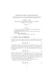
Algorithmsfor Picture AnalysisLecture 18: Minimum-Length PolygonsConvex HullA set S is called convex if for any two points p, q of S the straightline segment pq is contained in S.The convex hull C(S) is the intersection of all of the halfspaces ofR n that contain S; it is the smallest convex set that contains S.A convex polygon (polyhedron) is a nonempty bounded set that isan intersection of finitely many half-planes (half-spaces).A simple polygon (shaded, having 20 vertices) and its convexhull which is a simple polygon with 5 vertives.Convex hull of a finite set of points. – The calculation of convexhulls is a basic procedure in geometry-related picture analysis.Page 1 February 2005

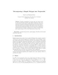
Algorithmsfor Picture AnalysisLecture 18: Minimum-Length PolygonsGraham’s ScanR.L Graham (1972): O(n log n) for n points in R 21. Start at a point of S (called the pivot p) that is knownto be on the convex hull.2. Sort the remaining points p i of S in order of increasingangles η i ; if the angle is the same for more thanone point, keep only the point furthest from p. Let theresulting sorted sequence of points be q 1 , . . . , q m .3. Initialize C(S) by the edge between p and q 1 .4. Scan through the sorted sequence. At each left turn,add a new edge to C(S); skip the point if there isno turn (a collinear situation); backtrack at each rightturn.Left: angles η i for the vectors defined by q 1 , q 2 , q 5 , q 4 . Right:backtrack situation at q 6 ; the dashed edges are removed or notadded in Step 4 of the algorithm.Page 2 February 2005

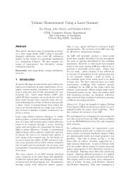
Algorithmsfor Picture AnalysisLecture 18: Minimum-Length PolygonsRelative Convex HullJ. Sklansky, R.L. Chazin, and B.J. Hansen in 1972Definition 1 Let S ⊆ B ⊂ R 2 . S is called B-convex iff, for allp, q ∈ S, if the straight line segment pq is in B, it is also in S. TheB-convex hull of S is the intersection of all B-convex sets that containS.Relative convex hulls. Left: A, B are simple polygons. Right:A, B are isothetic simple polygons.If A, B are simple polygons and A is contained in B, it can beshown that the frontier of the B-convex hull of A is the(uniquely determined) minimum-length polygonal curve (short:MLP) that is contained in B and that circumscribes A.Relative convex hulls are often used in robotics, computationalgeometry and picture analysis (digital geometry).Page 3 February 2005

Algorithmsfor Picture AnalysisLecture 18: Minimum-Length PolygonsLength in the 2D Cell Modelintrinsic distance between two points in a simple polygon = thelength of a shortest arc that connects the points and is containedin the polygonit follows: this is a polygonal arcintrinsic diameter of a polygon = the maximum intrinsic distancebetween any two of its pointsit follows: is between two vertices of the polygonLeft: the length of a simple 1-arc (in the 2D grid cell model) can bedefined by the length of its intrinsic diameterRight: the length of a simple 1-curve can be defined by the lengthof that MLP contained in the curve (to be precise: in the union ofall 2-cells of this curve), and circumscribing its “inner frontier”Page 4 February 2005

Algorithmsfor Picture AnalysisLecture 18: Minimum-Length PolygonsLength in the 3D Cell ModelLeft: the length of a simple 2-arc (in the 3D grid cell model) can bedefined by the length of its intrinsic diameterRight: the length of a simple 2-curve can be defined by the lengthof that MLP that is uniquely identified by being contained in thecurve and not contractible into a single point within this curve.Difference between 2D and 3DIn the 2D case, the MLP coincides with the relative convex hullof the “inner frontier” with respect to the “outer frontier” (andthe design of a 2D MLP algorithm is not very hard). In the 3Dcase, there is no such analogy with a relative convex hull (andthe calculation of a 3D MLP within a simple 2-curve is a difficulttask).Page 5 February 2005

Algorithmsfor Picture AnalysisLecture 18: Minimum-Length Polygons1-Curve around a Digital Regionpicture grid on the left: a 4-region and its frontier (bold curve)frontier grid on the right: the original frontier runs through pixelsin this grid, and we consider these as being 2-cells; the originalfrontier defines this way a 1-curve, which is not simple ingeneral, but can be used as input for an MLP algorithmassuming that the successor of a 2-cell in this 1-curve defines theonly possible grid edge where the MLP can cross into a next2-cell (the figure on the right shows in bold grid edges whichare not allowed to cross)resulting MLP, approximating the frontier of the given 4-regionPage 6 February 2005

Algorithmsfor Picture AnalysisLecture 18: Minimum-Length PolygonsSelf-Intersectionswe illustrate possible self-intersections of the frontier of a givensimply-connected 4-regionAccordingly, the 1-curve of grid cells in the frontier grid,following a trace around the frontier, will also haveself-intersections. The MLP-algorithm needs to handle thesecases as well. The figure illustrates (upper row) the repeatedvisit of one 2-cell, and (lower row) the construction of the MLPin this case. The final result is shown at the bottom on the left.Page 7 February 2005

Algorithmsfor Picture AnalysisLecture 18: Minimum-Length PolygonsInner and Outer FrontierFollowing the given 1-curve in counter-clockwise orientation (ina righthand coordinate system), the sequence of 1-cells on theright form a 0-curve γ 1 of 1-cells (the “outer frontier” in case ofa simple 1-curve), and those on the left a 0-curve γ 2 of 1-cells(the “inner frontier”).vertex v i on γ 1 or γ 2 is called a convex vertex if the frontier makesa positive turn at v i , detectable byD(v i−1 , v i , v i+1 ) > 0, where D is the determinantx 1 y 1 1x 2 y 2 1∣x 3 y 3 1∣ = x 1y 2 + x 3 y 1 + x 2 y 3 − x 3 y 2 − x 2 y 1 − x 1 y 3v i is called a concave vertex if the frontier makes a negative turn(D(v i−1 , v i , v i+1 ) < 0); a collinear vertex if D(v i−1 , v i , v i+1 ) = 0Our algorithm traces γ 1 (or γ 2 ), detects convex and concavevertices, puts their coordinates into a list L, and marks them asconvex or concave.For simplicity assume that the coordinates are integers; thecoordinates of two successive vertices with indices i and i + 1satisfy |x i+1 − x i | + |y i+1 − y i | = 1.Only convex vertices of the inner curve γ 2 and only concavevertices of the outer curve γ 1 can be vertices of the MLP.Page 8 February 2005

Algorithmsfor Picture AnalysisLecture 18: Minimum-Length PolygonsThere exists a mapping from the set of all concave vertices of γ 2onto the set of all concave vertices of γ 1 such that each concavevertex of γ 1 corresponds to at least one concave vertex of γ 2 .Numbers in the figure denote successive vertices in the list L:1 is a start vertex (i.e., an already known MLP vertex); 3 and 5are successive convex vertices on γ 2 ; 2, 4, and 6 are successiveconcave vertices on γ 1 . Vertex 7 is not between the negative(black line) and positive (white line) sides of sector (6,1,5);therefore 5 is the next MLP vertex and is a new start vertex.Start: put all of the vertices of γ 2 into L, then replace eachconcave vertex of γ 2 in L with its corresponding concave vertexof γ 1 by modifying its coordinates by ±1, where the signdepends on the orientations of the incident edges.L = all (plus others) of the vertices that will form the MLPPage 9 February 2005

Algorithmsfor Picture AnalysisLecture 18: Minimum-Length PolygonsMLP calculation and calculation of its length L1. Initialize list L = (v 1 , . . . , v n ) as described above; itcontains all of the vertices on γ 2 except the concavevertices, which are replaced by concave vertices on γ 1 .Each v i in L is labeled by the sign of D(v i−1 , v i , v i+1 ).2. Let k := 1, a := 1, b := 1 and i := 2. Let L := 0 andp 1 := v 1 .//v 1 is the first MLP vertex//3. If i > n + 1, stop.4. If i ≤ n, then j := i; else j := 1. //go back to v 1 //5. If D(p k , v b , v j ) > 0, then //v j lies on the positiveside//{k := k + 1, p k := v b , i := b, a := b, and L :=L + d e (p k−1 , p k )};else(a) If D(p k , v a , v j ) ≥ 0, then //v j is in the sector//;if v j has a positive label, then b := j, else a := j;else //v j lies on the negative side//(b) {k := k + 1, p k := v a , i := a, b := a, and L :=L + d e (p k−1 , p k )}6. Let i := i + 1 and go to Step 3.The algorithm has linear time complexity.Page 10 February 2005

Algorithmsfor Picture AnalysisLecture 18: Minimum-Length PolygonsSuppose we already know that vertex v i of L is an MLP vertex.Then v j (j > i) can be an MLP vertex only if all convex verticesv + k such that i < k < j lie on the positive side of (v i, v j ) or arecollinear with it (i.e., D(v i , v + k , v j) ≥ 0).Similarly, all concave vertices v − lsuch that i < l < j must lie onthe negative side of (v i , v j ) or be collinear with it.Suppose a convex vertex v + and a concave vertex v − bothsatisfy these conditions. When we consider a vertex v as acandidate MLP vertex, the following situations can occur:1. v lies on the positive side of (v i , v + ) (i.e., D(v i , v + , v) ≥ 0);2. v lies on the negative side of (v i , v + ) or is collinear with itand also lies on the positive side of (v i , v − ) or is collinearwith it; or3. v lies on the negative side of (v i , v − ).In case (1), v + becomes the next MLP vertex.In case (2), v becomes a candidate for the MLP and must replaceeither v + or v − depending on the sign of v.In case (3), v − becomes the next MLP vertex. This is also correctin the trivial case where v + , v − , or both coincide with v i .Start: a vertex v 1 that is known to be an MLP vertex (e.g., theuppermost-leftmost vertex of γ 2 ); set v + and v − equal to v 1 ; andthen test all subsequent vertices as just described.Whenever the next MLP vertex is detected, it becomes a newstart vertex.Page 11 February 2005

Algorithmsfor Picture AnalysisLecture 18: Minimum-Length PolygonsCourseworkRelated material in textbook: Sections 1.2.9, 10.1.4, 10.2.3, and10.2.4.A.18. [7 marks] Implement the given MLP algorithm forestimating the perimeter of a simply-connected 4-region by thelength of the MLP. (The calculated length L defines the lengthestimator E mlp .) Note:http://www.citr.auckland.ac.nz/dgt/Source Code.php?id=4offers a free download of an MLP source.Allow as input simply-connected 4-regions of arbitrary shapeand size in a 256 × 256 binary picture.(i) Test your algorithm by considering “extreme input cases”,such as shown below.(ii) Generate a diagram which shows run-times of youralgorithm in dependence upon the length of the frontier (note:this length is equal to the number of 1-cells on this curve) of thegiven 4-region.(iii) Optionally, [1 mark] also provide a way (e.g., in a grid ofhigher resolution) to visualize the calculated MLP.Page 12 February 2005

Relative Convex Hull; MLP Approximation of Borders - CITR

Create successful ePaper yourself

Delete template?

Save as template?