

Numerical Methods in Quantum Mechanics - Dipartimento di Fisica
Numerical Methods in Quantum Mechanics - Dipartimento di Fisica
Numerical Methods in Quantum Mechanics - Dipartimento di Fisica

You also want an ePaper? Increase the reach of your titles
YUMPU automatically turns print PDFs into web optimized ePapers that Google loves.
Lecture notes<br />
<strong>Numerical</strong> <strong>Methods</strong> <strong>in</strong><br />
<strong>Quantum</strong> <strong>Mechanics</strong><br />
Corso <strong>di</strong> Laurea Magistrale <strong>in</strong> <strong>Fisica</strong><br />
Interateneo Trieste – Ud<strong>in</strong>e<br />
Anno accademico 2012/2013<br />
Paolo Giannozzi<br />
University of Ud<strong>in</strong>e<br />
Conta<strong>in</strong>s software and material written by<br />
Furio Ercolessi 1 and Stefano de Gironcoli 2<br />
1 Formerly at University of Ud<strong>in</strong>e<br />
2 SISSA - Trieste<br />
Last mo<strong>di</strong>fied May 23, 2013
Contents<br />
Introduction 1<br />
0.1 About Software . . . . . . . . . . . . . . . . . . . . . . . . . . . . 1<br />
0.1.1 Compilers . . . . . . . . . . . . . . . . . . . . . . . . . . . 1<br />
0.1.2 Visualization Tools . . . . . . . . . . . . . . . . . . . . . . 2<br />
0.1.3 Mathematical Libraries . . . . . . . . . . . . . . . . . . . 2<br />
0.1.4 Pitfalls <strong>in</strong> C-Fortran <strong>in</strong>terlanguage calls . . . . . . . . . . 3<br />
0.2 Bibliography . . . . . . . . . . . . . . . . . . . . . . . . . . . . . 4<br />
1 One-<strong>di</strong>mensional Schröd<strong>in</strong>ger equation 5<br />
1.1 The harmonic oscillator . . . . . . . . . . . . . . . . . . . . . . . 5<br />
1.1.1 Units . . . . . . . . . . . . . . . . . . . . . . . . . . . . . 6<br />
1.1.2 Exact solution . . . . . . . . . . . . . . . . . . . . . . . . 6<br />
1.1.3 Comparison with classical probability density . . . . . . . 8<br />
1.2 <strong>Quantum</strong> mechanics and numerical codes: some observations . . 9<br />
1.2.1 Quantization . . . . . . . . . . . . . . . . . . . . . . . . . 9<br />
1.2.2 A pitfall: pathological asymptotic behavior . . . . . . . . 9<br />
1.3 Numerov’s method . . . . . . . . . . . . . . . . . . . . . . . . . . 10<br />
1.3.1 Code: harmonic0 . . . . . . . . . . . . . . . . . . . . . . . 12<br />
1.3.2 Code: harmonic1 . . . . . . . . . . . . . . . . . . . . . . . 13<br />
1.3.3 Laboratory . . . . . . . . . . . . . . . . . . . . . . . . . . 15<br />
2 Schröd<strong>in</strong>ger equation for central potentials 16<br />
2.1 Variable separation . . . . . . . . . . . . . . . . . . . . . . . . . . 16<br />
2.1.1 Ra<strong>di</strong>al equation . . . . . . . . . . . . . . . . . . . . . . . . 18<br />
2.2 Coulomb potential . . . . . . . . . . . . . . . . . . . . . . . . . . 18<br />
2.2.1 Energy levels . . . . . . . . . . . . . . . . . . . . . . . . . 20<br />
2.2.2 Ra<strong>di</strong>al wave functions . . . . . . . . . . . . . . . . . . . . 20<br />
2.3 Code: hydrogen ra<strong>di</strong>al . . . . . . . . . . . . . . . . . . . . . . . . 21<br />
2.3.1 Logarithmic grid . . . . . . . . . . . . . . . . . . . . . . . 21<br />
2.3.2 Improv<strong>in</strong>g convergence with perturbation theory . . . . . 22<br />
2.3.3 Laboratory . . . . . . . . . . . . . . . . . . . . . . . . . . 24<br />
3 Scatter<strong>in</strong>g from a potential 25<br />
3.1 Short rem<strong>in</strong>der of the theory of scatter<strong>in</strong>g . . . . . . . . . . . . . 25<br />
3.2 Scatter<strong>in</strong>g of H atoms from rare gases . . . . . . . . . . . . . . . 27<br />
3.2.1 Derivation of Van der Waals <strong>in</strong>teraction . . . . . . . . . . 27<br />
i
3.3 Code: crossection . . . . . . . . . . . . . . . . . . . . . . . . . . . 28<br />
3.3.1 Laboratory . . . . . . . . . . . . . . . . . . . . . . . . . . 30<br />
4 The Variational Method 32<br />
4.1 Variational Pr<strong>in</strong>ciple . . . . . . . . . . . . . . . . . . . . . . . . . 32<br />
4.1.1 Demonstration of the variational pr<strong>in</strong>ciple . . . . . . . . . 32<br />
4.1.2 Alternative demonstration of the variational pr<strong>in</strong>ciple . . 33<br />
4.1.3 Ground state energy . . . . . . . . . . . . . . . . . . . . . 34<br />
4.1.4 Variational method <strong>in</strong> practice . . . . . . . . . . . . . . . 35<br />
4.2 Secular problem . . . . . . . . . . . . . . . . . . . . . . . . . . . . 35<br />
4.2.1 Expansion <strong>in</strong>to a basis set of orthonormal functions . . . 36<br />
4.3 Plane-wave basis set . . . . . . . . . . . . . . . . . . . . . . . . . 38<br />
4.4 Code: pwell . . . . . . . . . . . . . . . . . . . . . . . . . . . . . . 39<br />
4.4.1 Diagonalization rout<strong>in</strong>es . . . . . . . . . . . . . . . . . . . 40<br />
4.4.2 Laboratory . . . . . . . . . . . . . . . . . . . . . . . . . . 41<br />
5 Non-orthonormal basis sets 42<br />
5.1 Non-orthonormal basis set . . . . . . . . . . . . . . . . . . . . . . 42<br />
5.1.1 Gaussian functions . . . . . . . . . . . . . . . . . . . . . . 44<br />
5.1.2 Exponentials . . . . . . . . . . . . . . . . . . . . . . . . . 44<br />
5.2 Code: hydrogen gauss . . . . . . . . . . . . . . . . . . . . . . . . 44<br />
5.2.1 Laboratory . . . . . . . . . . . . . . . . . . . . . . . . . . 46<br />
6 Self-consistent Field 47<br />
6.1 The Hartree Approximation . . . . . . . . . . . . . . . . . . . . . 47<br />
6.2 Hartree Equations . . . . . . . . . . . . . . . . . . . . . . . . . . 48<br />
6.2.1 Eigenvalues and Hartree energy . . . . . . . . . . . . . . . 49<br />
6.3 Self-consistent potential . . . . . . . . . . . . . . . . . . . . . . . 50<br />
6.3.1 Self-consistent potential <strong>in</strong> atoms . . . . . . . . . . . . . . 50<br />
6.4 Code: helium hf ra<strong>di</strong>al . . . . . . . . . . . . . . . . . . . . . . . . 51<br />
6.4.1 Laboratory . . . . . . . . . . . . . . . . . . . . . . . . . . 52<br />
7 The Hartree-Fock approximation 53<br />
7.1 Hartree-Fock method . . . . . . . . . . . . . . . . . . . . . . . . . 53<br />
7.1.1 Coulomb and exchange potentials . . . . . . . . . . . . . . 55<br />
7.1.2 Correlation energy . . . . . . . . . . . . . . . . . . . . . . 56<br />
7.1.3 The Helium atom . . . . . . . . . . . . . . . . . . . . . . . 57<br />
7.2 Code: helium hf gauss . . . . . . . . . . . . . . . . . . . . . . . . 57<br />
7.2.1 Laboratory . . . . . . . . . . . . . . . . . . . . . . . . . . 59<br />
8 Molecules 60<br />
8.1 Born-Oppenheimer approximation . . . . . . . . . . . . . . . . . 60<br />
8.2 Potential Energy Surface . . . . . . . . . . . . . . . . . . . . . . . 61<br />
8.3 Diatomic molecules . . . . . . . . . . . . . . . . . . . . . . . . . . 62<br />
8.4 Code: h2 hf gauss . . . . . . . . . . . . . . . . . . . . . . . . . . 63<br />
8.4.1 Gaussian <strong>in</strong>tegrals . . . . . . . . . . . . . . . . . . . . . . 63<br />
8.4.2 Laboratory . . . . . . . . . . . . . . . . . . . . . . . . . . 64<br />
ii
9 Electrons <strong>in</strong> a perio<strong>di</strong>c potential 66<br />
9.1 Crystall<strong>in</strong>e solids . . . . . . . . . . . . . . . . . . . . . . . . . . . 66<br />
9.1.1 Perio<strong>di</strong>c Boundary Con<strong>di</strong>tions . . . . . . . . . . . . . . . 67<br />
9.1.2 Bloch Theorem . . . . . . . . . . . . . . . . . . . . . . . . 68<br />
9.1.3 The empty potential . . . . . . . . . . . . . . . . . . . . . 68<br />
9.1.4 Solution for the crystal potential . . . . . . . . . . . . . . 69<br />
9.1.5 Plane-wave basis set . . . . . . . . . . . . . . . . . . . . . 70<br />
9.2 Code: perio<strong>di</strong>cwell . . . . . . . . . . . . . . . . . . . . . . . . . . 72<br />
9.2.1 Laboratory . . . . . . . . . . . . . . . . . . . . . . . . . . 73<br />
10 Pseudopotentials 74<br />
10.1 Three-<strong>di</strong>mensional crystals . . . . . . . . . . . . . . . . . . . . . . 74<br />
10.2 Plane waves, core states, pseudopotentials . . . . . . . . . . . . . 75<br />
10.3 Code: cohenbergstresser . . . . . . . . . . . . . . . . . . . . . . . 76<br />
10.3.1 Laboratory . . . . . . . . . . . . . . . . . . . . . . . . . . 78<br />
11 Exact <strong>di</strong>agonalization of quantum sp<strong>in</strong> models 79<br />
11.1 The Heisenberg model . . . . . . . . . . . . . . . . . . . . . . . . 79<br />
11.2 Hilbert space <strong>in</strong> sp<strong>in</strong> systems . . . . . . . . . . . . . . . . . . . . 80<br />
11.3 Iterative <strong>di</strong>agonalization . . . . . . . . . . . . . . . . . . . . . . . 81<br />
11.4 Code: heisenberg exact . . . . . . . . . . . . . . . . . . . . . . 82<br />
11.4.1 Computer Laboratory . . . . . . . . . . . . . . . . . . . . 83<br />
A From two-body to one-body problem 85<br />
B Accidental degeneracy and dynamical symmetry 87<br />
C Composition of angular momenta: the coupled representation 88<br />
D Two-electron atoms 90<br />
D.1 Perturbative Treatment for Helium atom . . . . . . . . . . . . . . 91<br />
D.2 Variational treatment for Helium atom . . . . . . . . . . . . . . . 92<br />
D.3 ”Exact” treatment for Helium atom . . . . . . . . . . . . . . . . 93<br />
D.3.1 Laboratory . . . . . . . . . . . . . . . . . . . . . . . . . . 95<br />
E Useful algorithms 96<br />
E.1 Search of the zeros of a function . . . . . . . . . . . . . . . . . . 96<br />
E.1.1 Bisection method . . . . . . . . . . . . . . . . . . . . . . . 96<br />
E.1.2 Newton-Raphson method . . . . . . . . . . . . . . . . . . 97<br />
E.1.3 Secant method . . . . . . . . . . . . . . . . . . . . . . . . 97<br />
iii
Introduction<br />
The aim of these lecture notes is to provide an <strong>in</strong>troduction to methods and<br />
techniques used <strong>in</strong> the numerical solution of simple (non-relativistic) quantummechanical<br />
problems, with special emphasis on atomic and condensed-matter<br />
physics. The practical sessions are meant to be a sort of “computational laboratory”,<br />
<strong>in</strong>troduc<strong>in</strong>g the basic <strong>in</strong>gre<strong>di</strong>ents used <strong>in</strong> the calculation of materials<br />
properties at a much larger scale. The latter is a very important field of today’s<br />
computational physics, due to its technological <strong>in</strong>terest and potential applications.<br />
The codes provided dur<strong>in</strong>g the course are little more than templates. Students<br />
are expected to analyze them, to run them under various con<strong>di</strong>tions, to<br />
exam<strong>in</strong>e their behavior as a function of <strong>in</strong>put data, and most important, to<br />
<strong>in</strong>terpret their output from a physical po<strong>in</strong>t of view. The students will be asked<br />
to extend or mo<strong>di</strong>fy those codes, by add<strong>in</strong>g or mo<strong>di</strong>fy<strong>in</strong>g some functionalities.<br />
For further <strong>in</strong>sight on the theory of <strong>Quantum</strong> <strong>Mechanics</strong>, many excellent<br />
textbooks are available (e.g. Griffiths, Schiff, or the ever-green Dirac and Landau).<br />
For further <strong>in</strong>sight on the properly computational aspects of this course,<br />
we refer to the specialized texts quotes <strong>in</strong> the Bibliography section, and <strong>in</strong><br />
particular to the book of Thijssen.<br />
0.1 About Software<br />
This course assumes some basic knowledge of how to write and execute simple<br />
programs, and how to plot their results. All that is needed is a fortran or C<br />
compiler and some visualization software. The target mach<strong>in</strong>e is a PC runn<strong>in</strong>g<br />
L<strong>in</strong>ux, but other operat<strong>in</strong>g systems can be used as well (<strong>in</strong>clud<strong>in</strong>g Mac OS-X<br />
and W<strong>in</strong>dows), as long as the mentioned software is <strong>in</strong>stalled and work<strong>in</strong>g, and<br />
if you know how to use it <strong>in</strong> oractise.<br />
0.1.1 Compilers<br />
In order to run a code written <strong>in</strong> any programm<strong>in</strong>g language, we must first<br />
translate it <strong>in</strong>to mach<strong>in</strong>e language, i.e. a language that the computer can<br />
understand. The translation is done by an <strong>in</strong>terpreter or by a compiler: the<br />
former translates and imme<strong>di</strong>ately executes each <strong>in</strong>struction, the latter takes<br />
the file, produces the so-called object code that together with other object codes<br />
and with libraries is f<strong>in</strong>ally assembled <strong>in</strong>to an executable file. Python, Java (or at<br />
1
an higher level, Matlab, Mathematica) are examples of “<strong>in</strong>terpreted” language.<br />
Fortran, C, C++ are “compiled” languages.<br />
Our codes are written <strong>in</strong> Fortran 90. This is a sophisticated and complex<br />
language offer<strong>in</strong>g dynamical memory management, arrays operations (e.g.<br />
matrix-vector products), modular and object-based structure. Fortran 90 however<br />
can be as efficient as Fortran 77 and ma<strong>in</strong>ta<strong>in</strong>s a wide compatibility with<br />
exist<strong>in</strong>g Fortran 77 codes. It is worth mention<strong>in</strong>g that the first applications<br />
of computers to physics go back to well before the birth of modern computer<br />
languages like C++, python, or even C: there is still a large number of codes<br />
and libraries written <strong>in</strong> Fortran 77 (or even Fortran 66!) widely used <strong>in</strong> physics.<br />
Fortran 90 (or even Fortran 77, <strong>in</strong> this respect) is not a well known language.<br />
There are however many available resources (see for <strong>in</strong>stance the web page<br />
mentioned <strong>in</strong> the bibliography section) and the codes themselves are very simple<br />
and make little usage of advanced language features. In any case, there are no<br />
objections if a student prefers to use a more widespread language like C. A<br />
version of all codes <strong>in</strong> C is also available (no warranty about the quality of the<br />
C code <strong>in</strong> terms of elegance and good cod<strong>in</strong>g practice).<br />
In all cases, we need a C or Fortran 90 compiler. In PCs runn<strong>in</strong>g L<strong>in</strong>ux, the<br />
C compiler gcc is basically part of the operat<strong>in</strong>g system and is always present.<br />
Recent versions of gcc also <strong>in</strong>clude a Fortran compiler, called gfortran. If this<br />
is absent, or it is not easy to <strong>in</strong>stall it, one can download the free and rather<br />
reliable compiler, g95 1 . It is possible to <strong>in</strong>stall on Mac OS-X and on W<strong>in</strong>dows<br />
either gcc with gfortran or g95.<br />
0.1.2 Visualization Tools<br />
Visualization of data produced by the codes (wave functions, charge densities,<br />
various other quantities) has a central role <strong>in</strong> the analysis and understand<strong>in</strong>g<br />
of the results. Code gnuplot can be used to make two-<strong>di</strong>mensional or three<strong>di</strong>mensional<br />
plots of data or of analytical expressions. gnuplot is open-source<br />
software, available for all operat<strong>in</strong>g systems and usually found pre-<strong>in</strong>stalled on<br />
L<strong>in</strong>ux PCs. An <strong>in</strong>troduction to gnuplot, with many l<strong>in</strong>ks to more resources,<br />
can be found here: http://www.gnuplot.<strong>in</strong>fo/help.html.<br />
Another software that can be used is xmgrace 2 . This is also open-source<br />
and highly portable, has a graphical user <strong>in</strong>terface and thus it is easier to use<br />
than gnuplot, whose syntax is not always easy to remember.<br />
0.1.3 Mathematical Libraries<br />
The usage of efficient mathematical libraries is crucial <strong>in</strong> “serious” calculations.<br />
Some of the codes use rout<strong>in</strong>es from the BLAS 3 (Basic L<strong>in</strong>ear Algebra Subprograms)<br />
library and from LAPACK 4 (L<strong>in</strong>ear Algebra PACKage). The latter<br />
1 http://www.g95.org<br />
2 http://plasma-gate.weizmann.ac.il/Grace<br />
3 http://www.netlib.org/blas<br />
4 http://www.netlib.org/lapack<br />
2
is an important and well-known library for all k<strong>in</strong>ds of l<strong>in</strong>ear algebra operations:<br />
solution of l<strong>in</strong>ear systems, eigenvalue problems, etc. LAPACK calls<br />
BLAS rout<strong>in</strong>es for all CPU-<strong>in</strong>tensive calculations. The latter are available <strong>in</strong><br />
highly optimized form for many <strong>di</strong>fferent architectures.<br />
BLAS and LAPACK rout<strong>in</strong>es are written <strong>in</strong> Fortran 77. BLAS and LA-<br />
PACK are often available <strong>in</strong> many operat<strong>in</strong>g systems and can be l<strong>in</strong>ked <strong>di</strong>rectly<br />
by the compiler by add<strong>in</strong>g -llapack -lblas. In the case of C compiler, it<br />
may be needed to add an underscore ( ) <strong>in</strong> the call<strong>in</strong>g program, as <strong>in</strong>: dsyev ,<br />
dgemm . This is due to <strong>di</strong>fferent C-Fortran conventions for the nam<strong>in</strong>g of “symbols”<br />
(i.e. compiled rout<strong>in</strong>es). Note that the C compiler may also need -lm to<br />
l<strong>in</strong>k general mathematical libraries (i.e. operations like the square root).<br />
0.1.4 Pitfalls <strong>in</strong> C-Fortran <strong>in</strong>terlanguage calls<br />
In ad<strong>di</strong>tion to the above-mentioned potential mismatches between C and Fortran<br />
nam<strong>in</strong>g conventions, there are a few more pitfalls one has to be aware of<br />
when Fortran 77 rout<strong>in</strong>es are called by C (or vice versa).<br />
• Fortran passes po<strong>in</strong>ters to subrout<strong>in</strong>es and functions; C passes values. In<br />
order to call a Fortran rout<strong>in</strong>e from C, all C variables appear<strong>in</strong>g <strong>in</strong> the<br />
call must be either po<strong>in</strong>ters or arrays.<br />
• In<strong>di</strong>ces of vectors and arrays start from 0 <strong>in</strong> C, from 1 <strong>in</strong> Fortran (unless<br />
<strong>di</strong>fferently specified <strong>in</strong> array declaration or allocation).<br />
• Matrices <strong>in</strong> C are stored <strong>in</strong> memory row-wise, that is: a[i][j+1] follows<br />
a[i][j] <strong>in</strong> memory. In Fortran, they are stored column-wise (the other<br />
way round!): a(i+1,j) follows a(i,j) <strong>in</strong> memory.<br />
An ad<strong>di</strong>tional problem is that C does not provide run-time allocatable matrices<br />
like Fortran does, but only fixed-<strong>di</strong>mension matrices and arrays of po<strong>in</strong>ters.<br />
The former are impractical, the latter are not usable as arguments to pass to<br />
Fortran. It would be possible, us<strong>in</strong>g either non-standard C syntax, or us<strong>in</strong>g<br />
C++ and the new command, to def<strong>in</strong>e dynamically allocated matrices similar<br />
to those used <strong>in</strong> Fortran. We have preferred for our simple C codes to “simulate”<br />
Fortran-style matrices (i.e. stored <strong>in</strong> memory column-wise) by mapp<strong>in</strong>g them<br />
onto one-<strong>di</strong>mensional C vectors.<br />
We remark that Fortran 90 has a more advanced way of pass<strong>in</strong>g arrays to<br />
subrout<strong>in</strong>es us<strong>in</strong>g “array descriptors”. The codes used <strong>in</strong> this course however do<br />
not make use of this possibility but use the old-style Fortran 77 way of pass<strong>in</strong>g<br />
arrays via po<strong>in</strong>ters.<br />
3
0.2 Bibliography<br />
J. M. Thijssen, Computational Physics, Cambridge University Press, Cambridge,<br />
1999. A second e<strong>di</strong>tion has appeared:<br />
http://www.cambridge.org/gb/knowledge/isbn/item1171410.<br />
F. J. Vesely, Computational Physics - An Introduction: Second E<strong>di</strong>tion, Kluwer,<br />
2001. Also see the author’s web page:<br />
http://www.ap.univie.ac.at/users/Franz.Vesely/cp0102/serious.html,<br />
conta<strong>in</strong><strong>in</strong>g parts of the accompany<strong>in</strong>g material.<br />
S. E. Koon<strong>in</strong> e D. C. Mere<strong>di</strong>th, Computational physics - Fortran Version,<br />
Ad<strong>di</strong>son-Wesley, 1990. See also Dawn Mere<strong>di</strong>th’s web page:<br />
http://pubpages.unh.edu/%7Edawnm/.<br />
Timothy H. Kaiser, A quick <strong>in</strong>troduction to advanced Fortran-90:<br />
http://www.sdsc.edu/%7Etkaiser/f90.html.<br />
4
Chapter 1<br />
One-<strong>di</strong>mensional Schröd<strong>in</strong>ger<br />
equation<br />
In this chapter we will start from the harmonic oscillator to <strong>in</strong>troduce a general<br />
numerical methodology to solve the one-<strong>di</strong>mensional, time-<strong>in</strong>dependent Schröd<strong>in</strong>ger<br />
equation. The analytical solution of the harmonic oscillator will be first<br />
derived and described. A specific <strong>in</strong>tegration algorithm (Numerov) will be used.<br />
The extension of the numerical methodology to other, more general types of<br />
potentials does not present any special <strong>di</strong>fficulty.<br />
For a particle of mass m under a potential V (x), the one-<strong>di</strong>mensional, time<strong>in</strong>dependent<br />
Schröd<strong>in</strong>ger equation is given by:<br />
− ¯h2 d 2 ψ<br />
+ V (x)ψ(x) = Eψ(x), (1.1)<br />
2m dx2 where ψ(x) is the wave function, <strong>in</strong> general complex, and ¯h is the Planck constant<br />
h <strong>di</strong>vided by 2π. In the follow<strong>in</strong>g we are focus<strong>in</strong>g on the <strong>di</strong>screte spectrum:<br />
the set of isolated energy values for which Eq.(1.1) has normalizable solutions,<br />
localized <strong>in</strong> space.<br />
1.1 The harmonic oscillator<br />
The harmonic oscillator is a fundamental problem <strong>in</strong> classical dynamics as well<br />
as <strong>in</strong> quantum mechanics. It represents the simplest model system <strong>in</strong> which<br />
attractive forces are present and is an important para<strong>di</strong>gm for all k<strong>in</strong>ds of vibrational<br />
phenomena. For <strong>in</strong>stance, the vibrations around equilibrium positions<br />
of a system of <strong>in</strong>teract<strong>in</strong>g particles may be described, via an appropriate coord<strong>in</strong>ate<br />
transformation, <strong>in</strong> terms of <strong>in</strong>dependent harmonic oscillators known as<br />
normal vibrational modes. The same holds <strong>in</strong> quantum mechanics. The study<br />
of the quantum oscillator allows a deeper understand<strong>in</strong>g of quantization and of<br />
its effects and of wave functions of bound states.<br />
In this chapter we will first rem<strong>in</strong>d the ma<strong>in</strong> results of the theory of the<br />
harmonic oscillator, then we will show how to set up a computer code that<br />
allows to numerically solve the Schröd<strong>in</strong>ger equation for the harmonic oscillator.<br />
The result<strong>in</strong>g code can be easily mo<strong>di</strong>fied and adapted to a <strong>di</strong>fferent (not simply<br />
5
quadratic) <strong>in</strong>teraction potential. This will allow to study problems that, unlike<br />
the harmonic oscillator, do not have a simple analytical solution.<br />
1.1.1 Units<br />
The Schröd<strong>in</strong>ger equation for a one-<strong>di</strong>mensional harmonic oscillator is, <strong>in</strong> usual<br />
notations:<br />
d 2 (<br />
ψ<br />
dx 2 = −2m ¯h 2 E − 1 )<br />
2 Kx2 ψ(x) (1.2)<br />
where K the force constant (the force on the mass be<strong>in</strong>g F = −Kx, proportional<br />
to the <strong>di</strong>splacement x and <strong>di</strong>rected towards the orig<strong>in</strong>). Classically such an<br />
oscillator has a frequency (angular frequency)<br />
√<br />
K<br />
ω =<br />
m . (1.3)<br />
It is convenient to work <strong>in</strong> a<strong>di</strong>mensional units. These are the units that will<br />
be used by the codes presented at the end of this chapter. Let us <strong>in</strong>troduce<br />
a<strong>di</strong>mensional variables ξ, def<strong>in</strong>ed as<br />
ξ =<br />
( mK<br />
¯h 2 ) 1/4<br />
x =<br />
(us<strong>in</strong>g Eq.(1.3) for ω), and ɛ, def<strong>in</strong>ed as<br />
( ) mω 1/2<br />
x (1.4)<br />
¯h<br />
ε = Ē hω . (1.5)<br />
By <strong>in</strong>sert<strong>in</strong>g these variables <strong>in</strong>to the Schröd<strong>in</strong>ger equation, we f<strong>in</strong>d<br />
d 2 ( )<br />
ψ<br />
dξ 2 = −2 ε − ξ2<br />
ψ(ξ) (1.6)<br />
2<br />
which is written <strong>in</strong> a<strong>di</strong>mensional units.<br />
1.1.2 Exact solution<br />
One can easily verify that for large ξ (such that ε can be neglected) the solutions<br />
of Eq.(1.6) must have an asymptotic behavior like<br />
ψ(ξ) ∼ ξ n e ±ξ2 /2<br />
(1.7)<br />
where n is any f<strong>in</strong>ite value. The + sign <strong>in</strong> the exponent must however be<br />
<strong>di</strong>scarded: it would give raise to <strong>di</strong>verg<strong>in</strong>g, non-physical solutions (<strong>in</strong> which the<br />
particle would tend to leave the ξ = 0 po<strong>in</strong>t, <strong>in</strong>stead of be<strong>in</strong>g attracted towards<br />
it by the elastic force). It is thus convenient to extract the asymptotic behavior<br />
and assume<br />
ψ(ξ) = H(ξ)e −ξ2 /2<br />
(1.8)<br />
where H(ξ) is a well-behaved function for large ξ (i.e. the asymptotic behavior<br />
is determ<strong>in</strong>ed by the second factor e −ξ2 /2 ). In particular, H(ξ) must not grow<br />
like e ξ2 , or else we fall back <strong>in</strong>to a undesirable non-physical solution.<br />
6
Under the assumption of Eq.(1.8), Eq.(1.6) becomes an equation for H(ξ):<br />
H ′′ (ξ) − 2ξH ′ (ξ) + (2ε − 1)H(ξ) = 0. (1.9)<br />
It is imme<strong>di</strong>ate to notice that ε 0 = 1/2, H 0 (ξ) = 1 is the simplest solution.<br />
This is the ground state, i.e. the lowest-energy solution, as will soon be clear.<br />
In order to f<strong>in</strong>d all solutions, we expand H(ξ) <strong>in</strong>to a series (<strong>in</strong> pr<strong>in</strong>ciple an<br />
<strong>in</strong>f<strong>in</strong>ite one):<br />
∞∑<br />
H(ξ) = A n ξ n , (1.10)<br />
n=0<br />
we derive the series to f<strong>in</strong>d H ′ and H ′′ , plug the results <strong>in</strong>to Eq.(1.9) and regroup<br />
terms with the same power of ξ. We f<strong>in</strong>d an equation<br />
∞∑<br />
[(n + 2)(n + 1)A n+2 + (2ε − 2n − 1)A n ] ξ n = 0 (1.11)<br />
n=0<br />
that can be satisfied for any value of ξ only if the coefficients of all the orders<br />
are zero:<br />
(n + 2)(n + 1)A n+2 + (2ε − 2n − 1)A n = 0. (1.12)<br />
Thus, once A 0 and A 1 are given, Eq.(1.12) allows to determ<strong>in</strong>e by recursion the<br />
solution under the form of a power series.<br />
Let us assume that the series conta<strong>in</strong> an <strong>in</strong>f<strong>in</strong>ite number of terms. For large<br />
n, the coefficient of the series behave like<br />
A n+2<br />
A n<br />
→ 2 n , that is: A n+2 ∼ 1<br />
(n/2)! . (1.13)<br />
Remember<strong>in</strong>g that exp(ξ 2 ) = ∑ n ξ2n /n!, whose coefficient also behave as <strong>in</strong><br />
Eq.(1.13), we see that recursion relation Eq.(1.12) between coefficients produces<br />
a function H(ξ) that grows like exp(ξ 2 ), that is, produces unphysical <strong>di</strong>verg<strong>in</strong>g<br />
solutions.<br />
The only way to prevent this from happen<strong>in</strong>g is to have <strong>in</strong> Eq.(1.12) all<br />
coefficients beyond a given n vanish, so that the <strong>in</strong>f<strong>in</strong>ite series reduces to a<br />
f<strong>in</strong>ite-degree polynomial. This happens if and only if<br />
ε = n + 1 2<br />
(1.14)<br />
where n is a non-negative <strong>in</strong>teger.<br />
Allowed energies for the harmonic oscillator are thus quantized:<br />
(<br />
E n = n + 1 )<br />
¯hω n = 0, 1, 2, . . . (1.15)<br />
2<br />
The correspond<strong>in</strong>g polynomials H n (ξ) are known as Hermite polynomials. H n (ξ)<br />
is of degree n <strong>in</strong> ξ, has n nodes, is even [H n (−ξ) = H n (ξ)] for even n, odd<br />
[H n (−ξ) = −H n (ξ)] for odd n. S<strong>in</strong>ce e −ξ2 /2 is node-less and even, the complete<br />
wave function correspond<strong>in</strong>g to the energy E n :<br />
ψ n (ξ) = H n (ξ)e −ξ2 /2<br />
(1.16)<br />
7
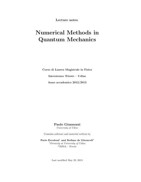
Figure 1.1: Wave functions and probability density for the quantum harmonic<br />
oscillator.<br />
has n nodes and the same parity as n. The fact that all solutions of the<br />
Schröd<strong>in</strong>ger equation are either odd or even functions is a consequence of the<br />
symmetry of the potential: V (−x) = V (x).<br />
The lowest-order Hermite polynomials are<br />
H 0 (ξ) = 1, H 1 (ξ) = 2ξ, H 2 (ξ) = 4ξ 2 − 2, H 3 (ξ) = 8ξ 3 − 12ξ. (1.17)<br />
A graph of the correspond<strong>in</strong>g wave functions and probability density is shown<br />
<strong>in</strong> fig. 1.1.<br />
1.1.3 Comparison with classical probability density<br />
The probability density for wave functions ψ n (x) of the harmonic oscillator<br />
have <strong>in</strong> general n + 1 peaks, whose height <strong>in</strong>creases while approach<strong>in</strong>g the<br />
correspond<strong>in</strong>g classical <strong>in</strong>version po<strong>in</strong>ts (i.e. po<strong>in</strong>ts where V (x) = E).<br />
These probability density can be compared to that of the classical harmonic<br />
oscillator, <strong>in</strong> which the mass moves accord<strong>in</strong>g to x(t) = x 0 s<strong>in</strong>(ωt). The probability<br />
ρ(x)dx to f<strong>in</strong>d the mass between x and x + dx is proportional to the time<br />
needed to cross such a region, i.e. it is <strong>in</strong>versely proportional to the speed as a<br />
function of x:<br />
ρ(x)dx ∝<br />
√<br />
S<strong>in</strong>ce v(t) = x 0 ω cos(ωt) = ω x 2 0 − x2 0 s<strong>in</strong>2 (ωt), we have<br />
ρ(x) ∝<br />
dx<br />
v(x) . (1.18)<br />
1<br />
√x 2 0 − x2 . (1.19)<br />
This probability density has a m<strong>in</strong>imum for x = 0, <strong>di</strong>verges at <strong>in</strong>version po<strong>in</strong>ts,<br />
is zero beyond <strong>in</strong>version po<strong>in</strong>ts.<br />
The quantum probability density for the ground state is completely <strong>di</strong>fferent:<br />
has a maximum for x = 0, decreases for <strong>in</strong>creas<strong>in</strong>g x. At the classical <strong>in</strong>version<br />
8
po<strong>in</strong>t its value is still ∼ 60% of the maximum value: the particle has a high<br />
probability to be <strong>in</strong> the classically forbidden region (for which V (x) > E).<br />
In the limit of large quantum numbers (i.e. large values of the <strong>in</strong>dex n),<br />
the quantum density tends however to look similar to the quantum one, but it<br />
still <strong>di</strong>splays the oscillatory behavior <strong>in</strong> the allowed region, typical for quantum<br />
systems.<br />
1.2 <strong>Quantum</strong> mechanics and numerical codes: some<br />
observations<br />
1.2.1 Quantization<br />
A first aspect to be considered <strong>in</strong> the numerical solution of quantum problems<br />
is the presence of quantization of energy levels for bound states, such as for<br />
<strong>in</strong>stance Eq.(1.15) for the harmonic oscillator. The acceptable energy values<br />
E n are not <strong>in</strong> general known a priori. Thus <strong>in</strong> the Schröd<strong>in</strong>ger equation (1.1)<br />
the unknown is not just ψ(x) but also E. For each allowed energy level, or<br />
eigenvalue, E n , there will be a correspond<strong>in</strong>g wave function, or eigenfunction,<br />
ψ n (x).<br />
What happens if we try to solve the Schröd<strong>in</strong>ger equation for an energy E<br />
that does not correspond to an eigenvalue? In fact, a “solution” exists for any<br />
value of E. We have however seen while study<strong>in</strong>g the harmonic oscillator that<br />
the quantization of energy orig<strong>in</strong>ates from boundary con<strong>di</strong>tions, requir<strong>in</strong>g no<br />
unphysical <strong>di</strong>vergence of the wave function <strong>in</strong> the forbidden regions. Thus, if<br />
E is not an eigenvalue, we will observe a <strong>di</strong>vergence of ψ(x). <strong>Numerical</strong> codes<br />
search<strong>in</strong>g for allowed energies must be able to recognize when the energy is not<br />
correct and search for a better energy, until it co<strong>in</strong>cides – with<strong>in</strong> numerical or<br />
predeterm<strong>in</strong>ed accuracy – with an eigenvalue. The first code presented at the<br />
end of this chapter implements such a strategy.<br />
1.2.2 A pitfall: pathological asymptotic behavior<br />
An important aspect of quantum mechanics is the existence of “negative” k<strong>in</strong>etic<br />
energies: i.e., the wave function can be non zero (and thus the probability<br />
to f<strong>in</strong>d a particle can be f<strong>in</strong>ite) <strong>in</strong> regions for which V (x) > E, forbidden accord<strong>in</strong>g<br />
to classical mechanics. Based on (1.1) and assum<strong>in</strong>g the simple case <strong>in</strong><br />
which V is (or can be considered) constant, this means<br />
d 2 ψ<br />
dx 2 = k2 ψ(x) (1.20)<br />
where k 2 is a positive quantity. This <strong>in</strong> turns implies an exponential behavior,<br />
with both ψ(x) ≃ exp(kx) and ψ(x) ≃ exp(−kx) satisfy<strong>in</strong>g (1.20). As a rule<br />
only one of these two possibilities has a physical mean<strong>in</strong>g: the one that gives<br />
raise to a wave function that decreases exponentially at large |x|.<br />
It is very easy to <strong>di</strong>st<strong>in</strong>guish between the “good” and the “bad” solution for<br />
a human. <strong>Numerical</strong> codes however are less good for such task: by their very<br />
nature, they accept both solutions, as long as they fulfill the equations. If even<br />
9
a t<strong>in</strong>y amount of the “bad” solution (due to numerical noise, for <strong>in</strong>stance) is<br />
present, the <strong>in</strong>tegration algorithm will <strong>in</strong>exorably make it grow <strong>in</strong> the classically<br />
forbidden region. As the <strong>in</strong>tegration goes on, the “bad” solution will sooner or<br />
later dom<strong>in</strong>ate the “good” one and eventually produce crazy numbers (or crazy<br />
NaN’s: Not a Number). Thus a nice-look<strong>in</strong>g wave function <strong>in</strong> the classically<br />
allowed region, smoothly decay<strong>in</strong>g <strong>in</strong> the classically forbidden region, may suddenly<br />
start to <strong>di</strong>verge beyond some limit, unless some wise strategy is employed<br />
to prevent it. The second code presented at the end of this chapter implements<br />
such a strategy.<br />
1.3 Numerov’s method<br />
Let us consider now the numerical solution of the (time-<strong>in</strong>dependent) Schröd<strong>in</strong>ger<br />
equation <strong>in</strong> one <strong>di</strong>mension. The basic assumption is that the equation<br />
can be <strong>di</strong>scretized, i.e. written on a suitable f<strong>in</strong>ite grid of po<strong>in</strong>ts, and <strong>in</strong>tegrated,<br />
i.e. solved, the solution be<strong>in</strong>g also given on the grid of po<strong>in</strong>ts.<br />
There are many big thick books on this subject, describ<strong>in</strong>g old and new<br />
methods, from the very simple to the very sophisticated, for all k<strong>in</strong>ds of <strong>di</strong>fferential<br />
equations and all k<strong>in</strong>ds of <strong>di</strong>scretizations and <strong>in</strong>tegration algorithms.<br />
In the follow<strong>in</strong>g, we will consider Numerov’s method (named after Russian astronomer<br />
Boris Vasilyevich Numerov) as an example of a simple yet powerful<br />
and accurate algorithm. Numerov’s method is useful to <strong>in</strong>tegrate second-order<br />
<strong>di</strong>fferential equations of the general form<br />
d 2 y<br />
= −g(x)y(x) + s(x) (1.21)<br />
dx2 where g(x) and s(x) are known functions. Initial con<strong>di</strong>tions for second-order<br />
<strong>di</strong>fferential equations are typically given as<br />
y(x 0 ) = y 0 , y ′ (x 0 ) = y ′ 0. (1.22)<br />
The Schröd<strong>in</strong>ger equation (1.1) has this form, with g(x) ≡ 2m [E − V (x)] and<br />
¯h 2<br />
s(x) = 0. We will see <strong>in</strong> the next chapter that also the ra<strong>di</strong>al Schröd<strong>in</strong>ger<br />
equations <strong>in</strong> three <strong>di</strong>mensions for systems hav<strong>in</strong>g spherical symmetry belongs<br />
to such class. Another important equation fall<strong>in</strong>g <strong>in</strong>to this category is Poisson’s<br />
equation of electromagnetism,<br />
d 2 φ<br />
= −4πρ(x) (1.23)<br />
dx2 where ρ(x) is the charge density. In this case g(x) = 0 and s(x) = −4πρ(x).<br />
Let us consider a f<strong>in</strong>ite box conta<strong>in</strong><strong>in</strong>g the system: for <strong>in</strong>stance, −x max ≤<br />
x ≤ x max , with x max large enough for our solutions to decay to negligibly small<br />
values. Let us <strong>di</strong>vide our f<strong>in</strong>ite box <strong>in</strong>to N small <strong>in</strong>tervals of equal size, ∆x<br />
wide. We call x i the po<strong>in</strong>ts of the grid so obta<strong>in</strong>ed, y i = y(x i ) the values of the<br />
unknown function y(x) on grid po<strong>in</strong>ts. In the same way we <strong>in</strong><strong>di</strong>cate by g i and<br />
s i the values of the (known) functions g(x) and s(x) <strong>in</strong> the same grid po<strong>in</strong>ts. In<br />
order to obta<strong>in</strong> a <strong>di</strong>scretized version of the <strong>di</strong>fferential equation (i.e. to obta<strong>in</strong><br />
10
an equation <strong>in</strong>volv<strong>in</strong>g f<strong>in</strong>ite <strong>di</strong>fferences), we expand y(x) <strong>in</strong>to a Taylor series<br />
around a po<strong>in</strong>t x n , up to fifth order:<br />
y n−1 =<br />
y n+1 =<br />
y n − y n∆x ′ + 1 2 y′′ n(∆x) 2 − 1 6 y′′′ n (∆x) 3 + 1<br />
+O[(∆x) 6 ]<br />
y n + y n∆x ′ + 1 2 y′′ n(∆x) 2 + 1 6 y′′′ n (∆x) 3 + 1<br />
+O[(∆x) 6 ].<br />
If we sum the two equations, we obta<strong>in</strong>:<br />
24 y′′′′<br />
24 y′′′′<br />
n (∆x) 4 − 1<br />
n (∆x) 4 + 1<br />
120 y′′′′′<br />
120 y′′′′′<br />
n (∆x) 5<br />
n (∆x) 5<br />
(1.24)<br />
y n+1 + y n−1 = 2y n + y ′′<br />
n(∆x) 2 + 1<br />
12 y′′′′ n (∆x) 4 + O[(∆x) 6 ]. (1.25)<br />
Eq.(1.21) tells us that<br />
y n ′′ = −g n y n + s n ≡ z n . (1.26)<br />
The quantity z n above is <strong>in</strong>troduced to simplify the notations. The follow<strong>in</strong>g<br />
relation holds:<br />
z n+1 + z n−1 = 2z n + z ′′<br />
n(∆x) 2 + O[(∆x) 4 ] (1.27)<br />
(this is the simple formula for <strong>di</strong>scretized second derivative, that can be obta<strong>in</strong>ed<br />
<strong>in</strong> a straightforward way by Taylor expansion up to third order) and thus<br />
y ′′′′<br />
n ≡ z ′′<br />
n = z n+1 + z n−1 − 2z n<br />
(∆x) 2 + O[(∆x) 2 ]. (1.28)<br />
By <strong>in</strong>sert<strong>in</strong>g back these results <strong>in</strong>to Eq.(1.25) one f<strong>in</strong>ds<br />
y n+1 = 2y n − y n−1 + (−g n y n + s n )(∆x) 2<br />
+ 1<br />
12 (−g n+1y n+1 + s n+1 − g n−1 y n−1 + s n−1 + 2g n y n − 2s n )(∆x) 2<br />
+O[(∆x) 6 ]<br />
(1.29)<br />
and f<strong>in</strong>ally the Numerov’s formula<br />
[<br />
] [<br />
] ]<br />
(∆x)<br />
y n+1 1 + g 2<br />
(∆x)<br />
n+1 = 2y n 1 − 5g 2<br />
(∆x)<br />
n − y n−1<br />
[1 + g 2<br />
n−1<br />
12<br />
12<br />
+(s n+1 + 10s n + s n−1 ) (∆x)2<br />
12<br />
+ O[(∆x) 6 ]<br />
12<br />
(1.30)<br />
that allows to obta<strong>in</strong> y n+1 start<strong>in</strong>g from y n and y n−1 , and recursively the function<br />
<strong>in</strong> the entire box, as long as the value of the function is known <strong>in</strong> the first<br />
two po<strong>in</strong>ts (note the <strong>di</strong>fference with “tra<strong>di</strong>tional” <strong>in</strong>itial con<strong>di</strong>tions, Eq.(1.22),<br />
<strong>in</strong> which the value at one po<strong>in</strong>t and the derivative <strong>in</strong> the same po<strong>in</strong>t is specified).<br />
It is of course possible to <strong>in</strong>tegrate both <strong>in</strong> the <strong>di</strong>rection of positive x and<br />
<strong>in</strong> the <strong>di</strong>rection of negative x. In the presence of <strong>in</strong>version symmetry, it will be<br />
sufficient to <strong>in</strong>tegrate <strong>in</strong> just one <strong>di</strong>rection.<br />
In our case—Schröd<strong>in</strong>ger equation—the s n terms are absent. It is convenient<br />
to <strong>in</strong>troduce an auxiliary array f n , def<strong>in</strong>ed as<br />
(∆x) 2<br />
f n ≡ 1 + g n<br />
12 , where g n = 2m<br />
¯h 2 [E − V (x n)]. (1.31)<br />
With<strong>in</strong> such assumption Numerov’s formula can be written as<br />
y n+1 = (12 − 10f n)y n − f n−1 y n−1<br />
f n+1<br />
. (1.32)<br />
11
1.3.1 Code: harmonic0<br />
Code harmonic0.f90 1 (or harmonic0.c 2 ) solves the Schröd<strong>in</strong>ger equation for<br />
the quantum harmonic oscillator, us<strong>in</strong>g the Numerov’s algorithm above described<br />
for <strong>in</strong>tegration, and search<strong>in</strong>g eigenvalues us<strong>in</strong>g the “shoot<strong>in</strong>g method”.<br />
The code uses the a<strong>di</strong>mensional units <strong>in</strong>troduced <strong>in</strong> (1.4).<br />
The shoot<strong>in</strong>g method is quite similar to the bisection procedure for the<br />
search of the zero of a function. The code looks for a solution ψ n (x) with a<br />
pre-determ<strong>in</strong>ed number n of nodes, at an energy E equal to the mid-po<strong>in</strong>t of the<br />
energy range [E m<strong>in</strong> , E max ], i.e. E = (E max + E m<strong>in</strong> )/2. The energy range must<br />
conta<strong>in</strong> the desired eigenvalue E n . The wave function is <strong>in</strong>tegrated start<strong>in</strong>g<br />
from x = 0 <strong>in</strong> the <strong>di</strong>rection of positive x; tt the same time, the number of nodes<br />
(i.e. of changes of sign of the function) is counted. If the number of nodes is<br />
larger than n, E is too high; if the number of nodes is smaller than n, E is too<br />
low. We then choose the lower half-<strong>in</strong>terval [E m<strong>in</strong> , E max = E], or the upper half<strong>in</strong>terval<br />
[E m<strong>in</strong> = E, E max ], respectively, select a new trial eigenvalue E <strong>in</strong> the<br />
mid-po<strong>in</strong>t of the new <strong>in</strong>terval, iterate the procedure. When the energy <strong>in</strong>terval<br />
is smaller than a pre-determ<strong>in</strong>ed threshold, we assume that convergence has<br />
been reached.<br />
For negative x the function is constructed us<strong>in</strong>g symmetry, s<strong>in</strong>ce ψ n (−x) =<br />
(−1) n ψ n (x). This is of course possible only because V (−x) = V (x), otherwise<br />
<strong>in</strong>tegration would have been performed on the entire <strong>in</strong>terval. The parity of the<br />
wave function determ<strong>in</strong>es the choice of the start<strong>in</strong>g po<strong>in</strong>ts for the recursion. For<br />
n odd, the two first po<strong>in</strong>ts can be chosen as y 0 = 0 and an arbitrary f<strong>in</strong>ite value<br />
for y 1 . For n even, y 0 is arbitrary and f<strong>in</strong>ite, y 1 is determ<strong>in</strong>ed by Numerov’s<br />
formula, Eq.(1.32), with f 1 = f −1 and y 1 = y −1 :<br />
The code prompts for some <strong>in</strong>put data:<br />
y 1 = (12 − 10f 0)y 0<br />
2f 1<br />
. (1.33)<br />
• the limit x max for <strong>in</strong>tegration (typical values: 5 ÷ 10);<br />
• the number N of grid po<strong>in</strong>ts (typical values range from hundreds to a few<br />
thousand); note that the grid po<strong>in</strong>t <strong>in</strong>dex actually runs from 0 to N, so<br />
that ∆x = x max /N;<br />
• the name of the file where output data is written;<br />
• the required number n of nodes (the code will stop if you give a negative<br />
number).<br />
F<strong>in</strong>ally the code prompts for a trial energy. You should answer 0 <strong>in</strong> order to<br />
search for an eigenvalue with n nodes. The code will start iterat<strong>in</strong>g on the<br />
energy, pr<strong>in</strong>t<strong>in</strong>g on standard output (i.e. at the term<strong>in</strong>al): iteration number,<br />
number of nodes found (on the positive x axis only), the current energy eigenvalue<br />
estimate. It is however possible to specify an energy (not necessarily an<br />
1 http://www.fisica.uniud.it/%7Egiannozz/Corsi/MQ/Software/F90/harmonic0.f90<br />
2 http://www.fisica.uniud.it/%7Egiannozz/Corsi/MQ/Software/C/harmonic0.c<br />
12
eigenvalue) to force the code to perform an <strong>in</strong>tegration at fixed energy and see<br />
the result<strong>in</strong>g wave function. It is useful for test<strong>in</strong>g purposes and to better understand<br />
how the eigenvalue search works (or doesn’t work). Note that <strong>in</strong> this<br />
case the required number of nodes will not be honored; however the <strong>in</strong>tegration<br />
will be <strong>di</strong>fferent for odd or even number of nodes, because the parity of n<br />
determ<strong>in</strong>es how the first two grid po<strong>in</strong>ts are chosen.<br />
The output file conta<strong>in</strong>s five columns: respectively, x, ψ(x), |ψ(x)| 2 , ρ cl (x)<br />
and V (x). ρ cl (x) is the classical probability density (normalized to 1) of the<br />
harmonic oscillator, given <strong>in</strong> Eq.(1.19). All these quantities can be plotted as a<br />
function of x us<strong>in</strong>g any plott<strong>in</strong>g program, such as gnuplot, shortly described <strong>in</strong><br />
the <strong>in</strong>troduction. Note that the code will prompt for a new value of the number<br />
of nodes after each calculation of the wave function: answer -1 to stop the code.<br />
If you perform more than one calculation, the output file will conta<strong>in</strong> the result<br />
for all of them <strong>in</strong> sequence. Also note that the wave function are written for<br />
the entire box, from −x max to x max .<br />
It will become quickly evident that the code “sort of” works: the results<br />
look good <strong>in</strong> the region where the wave function is not vanish<strong>in</strong>gly small, but<br />
<strong>in</strong>variably, the pathological behavior described <strong>in</strong> Sec.(1.2.2) sets up and wave<br />
functions <strong>di</strong>verge at large |x|. As a consequence, it is impossible to normalize<br />
the ψ(x). The code def<strong>in</strong>itely needs to be improved. The proper way to deal<br />
with such <strong>di</strong>fficulty is to f<strong>in</strong>d an <strong>in</strong>herently stable algorithm.<br />
1.3.2 Code: harmonic1<br />
Code harmonic1.f90 3 (or harmonic1.c 4 ) is the improved version of harmonic0<br />
that does not suffer from the problem of <strong>di</strong>vergence at large x.<br />
Two <strong>in</strong>tegrations are performed: a forward recursion, start<strong>in</strong>g from x = 0,<br />
and a backward one, start<strong>in</strong>g from x max . The eigenvalue is fixed by the con<strong>di</strong>tion<br />
that the two parts of the function match with cont<strong>in</strong>uous first derivative (as<br />
required for a physical wave function, if the potential is f<strong>in</strong>ite). The match<strong>in</strong>g<br />
po<strong>in</strong>t is chosen <strong>in</strong> correspondence of the classical <strong>in</strong>version po<strong>in</strong>t, x cl , i.e. where<br />
V (x cl ) = E. Such po<strong>in</strong>t depends upon the trial energy E. For a function<br />
def<strong>in</strong>ed on a f<strong>in</strong>ite grid, the match<strong>in</strong>g po<strong>in</strong>t is def<strong>in</strong>ed with an accuracy that is<br />
limited by the <strong>in</strong>terval between grid po<strong>in</strong>ts. In practice, one f<strong>in</strong>ds the <strong>in</strong>dex icl<br />
of the first grid po<strong>in</strong>t x c = icl∆x such that V (x c ) > E; the classical <strong>in</strong>version<br />
po<strong>in</strong>t will be located somewhere between x c − ∆x and x c .<br />
The outward <strong>in</strong>tegration is performed until grid po<strong>in</strong>t icl, yield<strong>in</strong>g a function<br />
ψ L (x) def<strong>in</strong>ed <strong>in</strong> [0, x c ]; the number n of changes of sign is counted <strong>in</strong> the<br />
same way as <strong>in</strong> harmonic0. If n is not correct the energy is adjusted (lowered<br />
if n too high, raised if n too low) as <strong>in</strong> harmonic0. We note that it is not<br />
needed to look for changes of sign beyond x c : <strong>in</strong> fact we know a priori that <strong>in</strong><br />
the classically forbidden region there cannot be any nodes (no oscillations, just<br />
decay<strong>in</strong>g solution).<br />
If the number of nodes is the expected one, the code starts to <strong>in</strong>tegrate<br />
<strong>in</strong>ward from the rightmost po<strong>in</strong>ts. Note the statement y(mesh) = dx: its only<br />
3 http://www.fisica.uniud.it/%7Egiannozz/Corsi/MQ/Software/F90/harmonic1.f90<br />
4 http://www.fisica.uniud.it/%7Egiannozz/Corsi/MQ/Software/C/harmonic1.c<br />
13
goal is to force solutions to be positive, s<strong>in</strong>ce the solution at the left of the<br />
match<strong>in</strong>g po<strong>in</strong>t is also positive. The value dx is arbitrary: the solution is<br />
anyway rescaled <strong>in</strong> order to be cont<strong>in</strong>uous at the match<strong>in</strong>g po<strong>in</strong>t. The code<br />
stopst the same <strong>in</strong>dex icl correspond<strong>in</strong>g to x c . We thus get a function ψ R (x)<br />
def<strong>in</strong>ed <strong>in</strong> [x c , x max ].<br />
In general, the two parts of the wave function have <strong>di</strong>fferent values <strong>in</strong> x c :<br />
ψ L (x c ) and ψ R (x c ). We first of all re-scale ψ R (x) by a factor ψ L (x c )/ψ R (x c ),<br />
so that the two functions match cont<strong>in</strong>uously <strong>in</strong> x c . Then, the whole function<br />
ψ(x) is renormalized <strong>in</strong> such a way that ∫ |ψ(x)| 2 dx = 1.<br />
Now comes the crucial po<strong>in</strong>t: the two parts of the function will have <strong>in</strong><br />
general a <strong>di</strong>scont<strong>in</strong>uity at the match<strong>in</strong>g po<strong>in</strong>t ψ ′ R (x c) − ψ ′ L (x c). This <strong>di</strong>fference<br />
should be zero for a good solution, but it will not <strong>in</strong> practice, unless we are<br />
really close to the good energy E = E n . The sign of the <strong>di</strong>fference allows us<br />
to understand whether E is too high or too low, and thus to apply aga<strong>in</strong> the<br />
bisection method to improve the estimate of the energy.<br />
In order to calculate the <strong>di</strong>scont<strong>in</strong>uity with good accuracy, we write the<br />
Taylor expansions:<br />
yi−1 L = yL i − y i<br />
′L ∆x + 1 2 y′′L i (∆x) 2 + O[(∆x) 3 ]<br />
yi+1 R = yR i + y i<br />
′R ∆x + 1 2 y′′R i (∆x) 2 + O[(∆x) 3 ]<br />
(1.34)<br />
For clarity, <strong>in</strong> the above equation i <strong>in</strong><strong>di</strong>cates the <strong>in</strong>dex icl. We sum the two<br />
Taylor expansions and obta<strong>in</strong>, not<strong>in</strong>g that yi L = yi R = y i , and that y i<br />
′′L = y i ′′R =<br />
y i ′′ = −g iy i as guaranteed by Numerov’s method:<br />
that is<br />
y L i−1 + y R i+1 = 2y i + (y ′R<br />
i − y ′L<br />
i )∆x − g i y i (∆x) 2 + O[(∆x) 3 ] (1.35)<br />
y i ′R − y i<br />
′L = yL i−1 + yR i+1 − [2 − g i(∆x) 2 ]y i<br />
+ O[(∆x) 2 ] (1.36)<br />
∆x<br />
or else, by us<strong>in</strong>g the notations as <strong>in</strong> (1.31),<br />
y i ′R − y i<br />
′L = yL i−1 + yR i+1 − (14 − 12f i)y i<br />
+ O[(∆x) 2 ] (1.37)<br />
∆x<br />
In this way the code calculated the <strong>di</strong>scont<strong>in</strong>uity of the first derivative. If the<br />
sign of y i ′R −y i<br />
′L is positive, the energy is too high (can you give an argument for<br />
this?) and thus we move to the lower half-<strong>in</strong>terval; if negative, the energy is too<br />
low and we move to the upper half <strong>in</strong>terval. As usual, convergence is declared<br />
when the size of the energy range has been reduced, by successive bisection, to<br />
less than a pre-determ<strong>in</strong>ed tolerance threshold.<br />
Dur<strong>in</strong>g the procedure, the code pr<strong>in</strong>ts on standard output a l<strong>in</strong>e for each<br />
iteration, conta<strong>in</strong><strong>in</strong>g: the iteration number; the number of nodes found (on the<br />
positive x axis only); if the number of nodes is the correct one, the <strong>di</strong>scont<strong>in</strong>uity<br />
of the derivative y i ′R − y i<br />
′L (zero if number of nodes not yet correct); the current<br />
estimate for the energy eigenvalue. At the end, the code writes the f<strong>in</strong>al wave<br />
function (this time, normalized to 1!) to the output file.<br />
14
1.3.3 Laboratory<br />
Here are a few h<strong>in</strong>ts for “numerical experiments” to be performed <strong>in</strong> the computer<br />
lab (or afterward), us<strong>in</strong>g both codes:<br />
• Calculate and plot eigenfunctions for various values of n. It may be<br />
useful to plot, together with eigenfunctions or eigenfunctions squared, the<br />
classical probability density, conta<strong>in</strong>ed <strong>in</strong> the fourth column of the output<br />
file. It will clearly show the classical <strong>in</strong>version po<strong>in</strong>ts. With gnuplot, e.g.:<br />
plot "filename" u 1:3 w l, "filename" u 1:4 w l<br />
(u = us<strong>in</strong>g, 1:3 = plot column3 vs column 1, w l = with l<strong>in</strong>es; the second<br />
”filename” can be replaced by ””).<br />
• Look at the wave functions obta<strong>in</strong>ed by specify<strong>in</strong>g an energy value not<br />
correspond<strong>in</strong>g to an eigenvalue. Notice the <strong>di</strong>fference between the results<br />
of harmonic0 and harmonic1 <strong>in</strong> this case.<br />
• Look at what happens when the energy is close to but not exactly an<br />
eigenvalue. Aga<strong>in</strong>, compare the behavior of the two codes.<br />
• Exam<strong>in</strong>e the effects of the parameters xmax, mesh. For a given ∆x, how<br />
large can be the number of nodes?<br />
• Verify how close you go to the exact results (notice that there is a convergence<br />
threshold on the energy <strong>in</strong> the code). What are the factors that<br />
affect the accuracy of the results?<br />
Possible code mo<strong>di</strong>fications and extensions:<br />
• Mo<strong>di</strong>fy the potential, keep<strong>in</strong>g <strong>in</strong>version symmetry. This will require very<br />
little changes to be done. You might for <strong>in</strong>stance consider a “double-well”<br />
potential described by the form:<br />
[ (x ) 4 ( ) x 2<br />
V (x) = ɛ − 2 + 1]<br />
, ɛ, δ > 0. (1.38)<br />
δ δ<br />
• Mo<strong>di</strong>fy the potential, break<strong>in</strong>g <strong>in</strong>version symmetry. You might consider<br />
for <strong>in</strong>stance the Morse potential:<br />
[<br />
]<br />
V (x) = D e −2ax − 2e −ax + 1 , (1.39)<br />
widely used to model the potential energy of a <strong>di</strong>atomic molecule. Which<br />
changes are needed <strong>in</strong> order to adapt the algorithm to cover this case?<br />
15
Chapter 2<br />
Schröd<strong>in</strong>ger equation for<br />
central potentials<br />
In this chapter we will extend the concepts and methods <strong>in</strong>troduced <strong>in</strong> the previous<br />
chapter for a one-<strong>di</strong>mensional problem to a specific and very important<br />
class of three-<strong>di</strong>mensional problems: a particle of mass m under a central potential<br />
V (r), i.e. depend<strong>in</strong>g only upon the <strong>di</strong>stance r from a fixed center. The<br />
Schröd<strong>in</strong>ger equation we are go<strong>in</strong>g to study <strong>in</strong> this chapter is thus<br />
Hψ(r) ≡<br />
[<br />
− ¯h2<br />
2m ∇2 + V (r)<br />
]<br />
ψ(r) = Eψ(r). (2.1)<br />
The problem of two <strong>in</strong>teract<strong>in</strong>g particles via a potential depend<strong>in</strong>g only upon<br />
their <strong>di</strong>stance, V (|r 1 − r 2 |), e.g. the Hydrogen atom, reduces to this case (see<br />
the Appen<strong>di</strong>x), with m equal to the reduced mass of the two particles.<br />
The general solution proceeds via the separation of the Schröd<strong>in</strong>ger equation<br />
<strong>in</strong>to an angular and a ra<strong>di</strong>al part. In this chapter we will be consider the<br />
numerical solution of the ra<strong>di</strong>al Schröd<strong>in</strong>ger equation. A non-uniform grid is<br />
<strong>in</strong>troduced and the ra<strong>di</strong>al Schröd<strong>in</strong>ger equation is transformed to an equation<br />
that can still be solved us<strong>in</strong>g Numerov’s method.<br />
2.1 Variable separation<br />
Let us <strong>in</strong>troduce a polar coord<strong>in</strong>ate system (r, θ, φ), where θ is the polar angle,<br />
φ the azimuthal one, and the polar axis co<strong>in</strong>cides with the z Cartesian axis.<br />
After some algebra, one f<strong>in</strong>ds the expression of the Laplacian operator:<br />
∇ 2 = 1 r 2 ∂<br />
∂r<br />
(<br />
r 2 ∂ ∂r<br />
)<br />
+<br />
1<br />
r 2 s<strong>in</strong> θ<br />
∂<br />
∂θ<br />
(<br />
s<strong>in</strong> θ ∂ ∂θ<br />
)<br />
+<br />
1<br />
r 2 s<strong>in</strong> 2 θ<br />
∂ 2<br />
∂φ 2 (2.2)<br />
It is convenient to <strong>in</strong>troduce the operator L 2 = L 2 x + L 2 y + L 2 z, the square of the<br />
angular momentum vector operator, L = −i¯hr × ∇. Both ⃗ L and L 2 act only<br />
on angular variables. In polar coord<strong>in</strong>ates, the explicit representation of L 2 is<br />
L 2 = −¯h 2 [<br />
1<br />
s<strong>in</strong> θ<br />
(<br />
∂<br />
s<strong>in</strong> θ ∂ )<br />
+ 1<br />
∂θ ∂θ s<strong>in</strong> 2 θ<br />
∂ 2 ]<br />
∂φ 2 . (2.3)<br />
16
The Hamiltonian can thus be written as<br />
(<br />
H = − ¯h2 1 ∂<br />
2m r 2 r 2 ∂ )<br />
+ L2<br />
+ V (r). (2.4)<br />
∂r ∂r 2mr2 The term L 2 /2mr 2 also appears <strong>in</strong> the analogous classical problem: the ra<strong>di</strong>al<br />
motion of a mass hav<strong>in</strong>g classical angular momentum L cl can be described by an<br />
effective ra<strong>di</strong>al potential ˆV (r) = V (r) + L 2 cl /2mr2 , where the second term (the<br />
“centrifugal potential”) takes <strong>in</strong>to account the effects of rotational motion. For<br />
high L cl the centrifugal potential “pushes” the equilibrium positions outwards.<br />
In the quantum case, both L 2 and one component of the angular momentum,<br />
for <strong>in</strong>stance L z :<br />
L z = −i¯h ∂<br />
(2.5)<br />
∂φ<br />
commute with the Hamiltonian, so L 2 and L z are conserved and H, L 2 , L z have<br />
a (complete) set of common eigenfunctions. We can thus use the eigenvalues of<br />
L 2 and L z to classify the states. Let us now proceed to the separation of ra<strong>di</strong>al<br />
and angular variables, as suggested by Eq.(2.4). Let us assume<br />
ψ(r, θ, φ) = R(r)Y (θ, φ). (2.6)<br />
After some algebra we f<strong>in</strong>d that the Schröd<strong>in</strong>ger equation can be split <strong>in</strong>to an<br />
angular and a ra<strong>di</strong>al equation. The solution of the angular equations are the<br />
spherical harmonics, known functions that are eigenstates of both L 2 and of<br />
L z :<br />
L z Y lm (θ, φ) = m¯hY lm (θ, φ), L 2 Y lm (θ, φ) = l(l + 1)¯h 2 Y lm (θ, φ) (2.7)<br />
(l ≥ 0 and m = −l, ..., l are <strong>in</strong>teger numbers).<br />
The ra<strong>di</strong>al equation is<br />
(<br />
− ¯h2 1 ∂<br />
2m r 2 ∂r<br />
r 2 ∂R nl<br />
∂r<br />
) [<br />
]<br />
+ V (r) + ¯h2 l(l + 1)<br />
2mr 2 R nl (r) = E nl R nl (r). (2.8)<br />
In general, the energy will depend upon l because the effective potential does;<br />
moreover, for a given l, we expect a quantization of the bound states (if exist<strong>in</strong>g)<br />
and we have <strong>in</strong><strong>di</strong>cated with n the correspond<strong>in</strong>g <strong>in</strong>dex.<br />
F<strong>in</strong>ally, the complete wave function will be<br />
ψ nlm (r, θ, φ) = R nl (r)Y lm (θ, φ) (2.9)<br />
The energy does not depend upon m. As already observed, m classifies the<br />
projection of the angular momentum on an arbitrarily chosen axis. Due to<br />
spherical symmetry of the problem, the energy cannot depend upon the orientation<br />
of the vector L, but only upon his modulus. An energy level E nl will<br />
then have a degeneracy 2l + 1 (or larger, if there are other observables that<br />
commute with the Hamiltonian and that we haven’t considered).<br />
17
2.1.1 Ra<strong>di</strong>al equation<br />
The probability to f<strong>in</strong>d the particle at a <strong>di</strong>stance between r and r + dr from the<br />
center is given by the <strong>in</strong>tegration over angular variables:<br />
∫<br />
|ψ nlm (r, θ, φ)| 2 rdθ r s<strong>in</strong> θ dφdr = |R nl | 2 r 2 dr = |χ nl | 2 dr (2.10)<br />
where we have <strong>in</strong>troduced the auxiliary function χ(r) as<br />
χ(r) = rR(r) (2.11)<br />
and exploited the normalization of the spherical harmonics:<br />
∫<br />
|Y lm (θ, φ)| 2 dθ s<strong>in</strong> θ dφ = 1 (2.12)<br />
(the <strong>in</strong>tegration is extended to all possible angles). As a consequence the normalization<br />
con<strong>di</strong>tion for χ is<br />
∫ ∞<br />
|χ nl (r)| 2 dr = 1 (2.13)<br />
0<br />
The function |χ(r)| 2 can thus be <strong>di</strong>rectly <strong>in</strong>terpreted as a ra<strong>di</strong>al (probability)<br />
density. Let us re-write the ra<strong>di</strong>al equation for χ(r) <strong>in</strong>stead of R(r). Its is<br />
straightforward to f<strong>in</strong>d that Eq.(2.8) becomes<br />
− ¯h2 d 2 [<br />
]<br />
χ<br />
2m dr 2 + V (r) + ¯h2 l(l + 1)<br />
2mr 2 − E χ(r) = 0. (2.14)<br />
We note that this equation is completely analogous to the Schröd<strong>in</strong>ger equation<br />
<strong>in</strong> one <strong>di</strong>mension, Eq.(1.1), for a particle under an effective potential:<br />
ˆV (r) = V (r) + ¯h2 l(l + 1)<br />
2mr 2 . (2.15)<br />
As already expla<strong>in</strong>ed, the second term is the centrifugal potential. The same<br />
methods used to f<strong>in</strong>d the solution of Eq.(1.1), and <strong>in</strong> particular, Numerov’s<br />
method, can be used to f<strong>in</strong>d the ra<strong>di</strong>al part of the eigenfunctions of the energy.<br />
2.2 Coulomb potential<br />
The most important and famous case is when V (r) is the Coulomb potential:<br />
V (r) = − Ze2<br />
4πɛ 0 r , (2.16)<br />
where e = 1.6021 × 10 −19 C is the electron charge, Z is the atomic number<br />
(number of protons <strong>in</strong> the nucleus), ɛ 0 = 8.854187817 × 10 −12 <strong>in</strong> MKSA units.<br />
Physicists tend to prefer the CGS system, <strong>in</strong> which the Coulomb potential is<br />
written as:<br />
V (r) = −Zq 2 e/r. (2.17)<br />
18
In the follow<strong>in</strong>g we will use q 2 e = e 2 /(4πɛ 0 ) so as to fall back <strong>in</strong>to the simpler<br />
CGS form.<br />
It is often practical to work with atomic units (a.u.): units of length are<br />
expressed <strong>in</strong> Bohr ra<strong>di</strong>i (or simply, “bohr”), a 0 :<br />
a 0 =<br />
¯h2<br />
m e q 2 e<br />
= 0.529177 Å = 0.529177 × 10 −10 m, (2.18)<br />
while energies are expressed <strong>in</strong> Rydberg (Ry):<br />
1 Ry = m eq 4 e<br />
2¯h 2 = 13.6058 eV. (2.19)<br />
when m e = 9.11 × 10 −31 Kg is the electron mass, not the reduced mass of<br />
the electron and the nucleus. It is straightforward to verify that <strong>in</strong> such units,<br />
¯h = 1, m e = 1/2, q 2 e = 2.<br />
We may also take the Hartree (Ha) <strong>in</strong>stead or Ry as unit of energy:<br />
1 Ha = 2 Ry = m eq 4 e<br />
¯h 2 = 27.212 eV (2.20)<br />
thus obta<strong>in</strong><strong>in</strong>g another set on atomic units, <strong>in</strong> which ¯h = 1, m e = 1, q e = 1.<br />
Beware! Never talk about ”atomic units” without first specify<strong>in</strong>g which ones.<br />
In the follow<strong>in</strong>g, the first set (”Rydberg” units) will be occasionally used.<br />
We note first of all that for small r the centrifugal potential is the dom<strong>in</strong>ant<br />
term <strong>in</strong> the potential. The behavior of the solutions for r → 0 will then be<br />
determ<strong>in</strong>ed by<br />
d 2 χ l(l + 1)<br />
≃<br />
dr2 r 2 χ(r) (2.21)<br />
yield<strong>in</strong>g χ(r) ∼ r l+1 , or χ(r) ∼ r −l . The second possibility is not physical<br />
because χ(r) is not allowed to <strong>di</strong>verge.<br />
For large r <strong>in</strong>stead we remark that bound states may be present only if<br />
E < 0: there will be a classical <strong>in</strong>version po<strong>in</strong>t beyond which the k<strong>in</strong>etic energy<br />
becomes negative, the wave function decays exponentially, only some energies<br />
can yield valid solutions. The case E > 0 corresponds <strong>in</strong>stead to a problem of<br />
electron-nucleus scatter<strong>in</strong>g, with propagat<strong>in</strong>g solutions and a cont<strong>in</strong>uum energy<br />
spectrum. In this chapter, the latter case will not be treated.<br />
The asymptotic behavior of the solutions for large r → ∞ will thus be<br />
determ<strong>in</strong>ed by<br />
d 2 χ<br />
dr 2 ≃ −2m e<br />
2<br />
Eχ(r) (2.22)<br />
¯h<br />
yield<strong>in</strong>g χ(r) ∼ exp(±kr), where k = √ −2m e E/¯h. The + sign must be <strong>di</strong>scarded<br />
as unphysical. It is thus sensible to assume for the solution a form<br />
like<br />
χ(r) = r l+1 e −kr<br />
∞ ∑<br />
n=0<br />
A n r n (2.23)<br />
which guarantees <strong>in</strong> both cases, small and large r, a correct behavior, as long<br />
as the series does not <strong>di</strong>verge exponentially.<br />
19
2.2.1 Energy levels<br />
The ra<strong>di</strong>al equation for the Coulomb potential can then be solved along the<br />
same l<strong>in</strong>es as for the harmonic oscillator, Sect.1.1. The expansion (2.23) is<br />
<strong>in</strong>troduced <strong>in</strong>to (2.14), a recursion formula for coefficients A n is derived, one<br />
f<strong>in</strong>ds that the series <strong>in</strong> general <strong>di</strong>verges like exp(2kr) unless it is truncated to a<br />
f<strong>in</strong>ite number of terms, and this happens only for some particular values of E:<br />
E n = − Z2<br />
n 2 m e q 4 e<br />
2¯h 2<br />
= − Z2<br />
Ry (2.24)<br />
n2 where n ≥ l + 1 is an <strong>in</strong>teger known as ma<strong>in</strong> quantum number. For a given l<br />
we f<strong>in</strong>d solutions for n = l + 1, l + 2, . . .; or, for a given n, possible values for l<br />
are l = 0, 1, . . . , n − 1.<br />
Although the effective potential appear<strong>in</strong>g <strong>in</strong> Eq.(2.14) depend upon l, and<br />
the angular part of the wave functions also strongly depend upon l, the energies<br />
(2.24) depend only upon n. We have thus a degeneracy on the energy levels<br />
with the same n and <strong>di</strong>fferent l, <strong>in</strong> ad<strong>di</strong>tion to the one due to the 2l+1 possible<br />
values of the quantum number m (as implied <strong>in</strong> (2.8) where m does not appear).<br />
The total degeneracy (not consider<strong>in</strong>g sp<strong>in</strong>) for a given n is thus<br />
n−1 ∑<br />
l=0<br />
2.2.2 Ra<strong>di</strong>al wave functions<br />
(2l + 1) = n 2 . (2.25)<br />
F<strong>in</strong>ally, the solution for the ra<strong>di</strong>al part of the wave functions is<br />
where<br />
χ nl (r) =<br />
√<br />
(n − l − 1)!Z<br />
n 2 [(n + l)!] 3 a 3 0<br />
x ≡ 2Z n<br />
x l+1 e −x/2 L 2l+1<br />
n+1 (x) (2.26)<br />
√<br />
r<br />
= 2 − 2m eE n<br />
a 0 ¯h 2 r (2.27)<br />
and L 2l+1<br />
n+1 (x) are Laguerre polynomials of degree n − l − 1. The coefficient has<br />
been chosen <strong>in</strong> such a way that the follow<strong>in</strong>g orthonormality relations hold:<br />
∫ ∞<br />
χ nl (r)χ n ′ l(r)dr = δ nn ′. (2.28)<br />
0<br />
The ground state has n = 1 and l = 0: 1s <strong>in</strong> “spectroscopic” notation (2p is<br />
n = 2, l = 1, 3d is n = 3, l = 2, 4f is n = 4, l = 3, and so on). For the Hydrogen<br />
atom (Z = 1) the ground state energy is −1Ry and the b<strong>in</strong>d<strong>in</strong>g energy of the<br />
electron is 1 Ry (apart from the small correction due to the <strong>di</strong>fference between<br />
electron mass and reduced mass). The wave function of the ground state is a<br />
simple exponential. With the correct normalization:<br />
ψ 100 (r, θ, φ) = Z3/2<br />
√ e −Zr/a 0<br />
. (2.29)<br />
π<br />
a 3/2<br />
0<br />
20
The dom<strong>in</strong>at<strong>in</strong>g term close to the nucleus is the first term of the series,<br />
χ nl (r) ∼ r l+1 . The larger l, the quicker the wave function tends to zero when<br />
approach<strong>in</strong>g the nucleus. This reflects the fact that the function is “pushed<br />
away” by the centrifugal potential. Thus ra<strong>di</strong>al wave functions with large l do<br />
not appreciably penetrate close to the nucleus.<br />
At large r the dom<strong>in</strong>at<strong>in</strong>g term is χ(r) ∼ r n exp(−Zr/na 0 ). This means<br />
that, neglect<strong>in</strong>g the other terms, |χ nl (r)| 2 has a maximum about r = n 2 a 0 /Z.<br />
This gives a rough estimate of the “size” of the wave function, which is ma<strong>in</strong>ly<br />
determ<strong>in</strong>ed by n.<br />
In Eq.(2.26) the polynomial has n − l − 1 degree. This is also the number of<br />
nodes of the function. In particular, the eigenfunctions with l = 0 have n − 1<br />
nodes; those with l = n − 1 are node-less. The form of the ra<strong>di</strong>al functions can<br />
be seen for <strong>in</strong>stance on the Wolfram Research site 1 or explored via the Java<br />
applet at Davidson College 2<br />
2.3 Code: hydrogen ra<strong>di</strong>al<br />
The code hydrogen ra<strong>di</strong>al.f90 3 or hydrogen ra<strong>di</strong>al.c 4 solves the ra<strong>di</strong>al equation<br />
for a one-electron atom. It is based on harmonic1, but solves a slightly<br />
<strong>di</strong>fferent equation on a logarithmically spaced grid. Moreover it uses a more<br />
sophisticated approach to locate eigenvalues, based on a perturbative estimate<br />
of the needed correction.<br />
The code uses atomic (Rydberg) units, so lengths are <strong>in</strong> Bohr ra<strong>di</strong>i (a 0 = 1),<br />
energies <strong>in</strong> Ry, ¯h 2 /(2m e ) = 1, q 2 e = 2.<br />
2.3.1 Logarithmic grid<br />
The straightforward numerical solution of Eq.(2.14) runs <strong>in</strong>to the problem of<br />
the s<strong>in</strong>gularity of the potential at r = 0. One way to circumvent this <strong>di</strong>fficulty<br />
is to work with a variable-step grid <strong>in</strong>stead of a constant-step one, as done until<br />
now. Such grid becomes denser and denser as we approach the orig<strong>in</strong>. “Serious”<br />
solutions of the ra<strong>di</strong>al Schröd<strong>in</strong>ger <strong>in</strong> atoms, especially <strong>in</strong> heavy atoms, <strong>in</strong>variably<br />
<strong>in</strong>volve such k<strong>in</strong>d of grids, s<strong>in</strong>ce wave functions close to the nucleus vary on<br />
a much smaller length scale than far from the nucleus. A detailed description of<br />
the scheme presented here can be found <strong>in</strong> chap.6 of The Hartree-Fock method<br />
for atoms, C. Froese Fischer, Wiley, 1977.<br />
Let us <strong>in</strong>troduce a new <strong>in</strong>tegration variable x and a constant-step grid <strong>in</strong><br />
x, so as to be able to use Numerov’s method without changes. We def<strong>in</strong>e a<br />
mapp<strong>in</strong>g between r and x via<br />
x = x(r). (2.30)<br />
The relation between the constant-step grid spac<strong>in</strong>g ∆x and the variable-step<br />
grid spac<strong>in</strong>g is given by<br />
∆x = x ′ (r)∆r. (2.31)<br />
1 http://library.wolfram.com/webMathematica/Physics/Hydrogen.jsp<br />
2 http://webphysics.davidson.edu/physlet resources/cise qm/html/hydrogenic.html<br />
3 http://www.fisica.uniud.it/%7Egiannozz/Corsi/MQ/Software/F90/hydrogen ra<strong>di</strong>al.f90<br />
4 http://www.fisica.uniud.it/%7Egiannozz/Corsi/MQ/Software/C/hydrogen ra<strong>di</strong>al.c<br />
21
We make the specific choice<br />
(note that with this choice x is a<strong>di</strong>mensional) yield<strong>in</strong>g<br />
x(r) ≡ log Zr<br />
a 0<br />
(2.32)<br />
∆x = ∆r<br />
r . (2.33)<br />
The ∆r/r ratio rema<strong>in</strong>s thus constant on the grid of r, called logarithmic grid,<br />
so def<strong>in</strong>ed.<br />
There is however a problem: by transform<strong>in</strong>g Eq.(2.14) <strong>in</strong> the new variable<br />
x, a term with first derivative appears, prevent<strong>in</strong>g the usage of Numerov’s<br />
method (and of other <strong>in</strong>tegration methods as well). The problem can be circumvented<br />
by transform<strong>in</strong>g the unknown function as follows:<br />
y(x) = 1 √ r<br />
χ (r(x)) . (2.34)<br />
It is easy to verify that by transform<strong>in</strong>g Eq.(2.14) so as to express it as a<br />
function of x and y, the terms conta<strong>in</strong><strong>in</strong>g first-order derivatives <strong>di</strong>sappear, and<br />
by multiply<strong>in</strong>g both sides of the equation by r 3/2 one f<strong>in</strong>ds<br />
d 2 [ (<br />
y<br />
dx 2 + 2me<br />
¯h 2 r2 (E − V (r)) − l + 1 ) ] 2<br />
y(x) = 0 (2.35)<br />
2<br />
where V (r) = −Zqe/r 2 for the Coulomb potential. This equation no longer<br />
presents any s<strong>in</strong>gularity for r = 0, is <strong>in</strong> the form of Eq.(1.21), with<br />
g(x) = 2m (<br />
e<br />
¯h 2 r(x)2 (E − V (r(x))) − l + 1 2<br />
(2.36)<br />
2)<br />
and can be <strong>di</strong>rectly solved us<strong>in</strong>g the numerical <strong>in</strong>tegration formulae Eqs.(1.31)<br />
and Eq.(1.32) and an algorithm very similar to the one of Sect.1.3.2.<br />
Subrout<strong>in</strong>e do mesh def<strong>in</strong>es at the beg<strong>in</strong>n<strong>in</strong>g and once for all the values of<br />
r, √ r, r 2 for each grid po<strong>in</strong>t. The potential is also calculated once and for all<br />
<strong>in</strong> <strong>in</strong>it pot. The grid is calculated start<strong>in</strong>g from a m<strong>in</strong>imum value x = −8,<br />
correspond<strong>in</strong>g to Zr m<strong>in</strong> ≃ 3.4 × 10 −3 Bohr ra<strong>di</strong>i. Note that the grid <strong>in</strong> r does<br />
not <strong>in</strong>clude r = 0: this would correspond to x = −∞. The known analytical<br />
behavior for r → 0 and r → ∞ are used to start the outward and <strong>in</strong>ward<br />
recurrences, respectively.<br />
2.3.2 Improv<strong>in</strong>g convergence with perturbation theory<br />
A few words are <strong>in</strong> order to expla<strong>in</strong> this section of the code:<br />
i = icl<br />
ycusp = (y(i-1)*f(i-1)+f(i+1)*y(i+1)+10.d0*f(i)*y(i)) / 12.d0<br />
dfcusp = f(i)*(y(i)/ycusp - 1.d0)<br />
! eigenvalue update us<strong>in</strong>g perturbation theory<br />
de = dfcusp/ddx12 * ycusp*ycusp * dx<br />
22
whose goal is to give an estimate, to first order <strong>in</strong> perturbation theory, of the<br />
<strong>di</strong>fference δe between the current estimate of the eigenvalue and its f<strong>in</strong>al value.<br />
Rem<strong>in</strong>der: icl is the <strong>in</strong>dex correspond<strong>in</strong>g to the classical <strong>in</strong>version po<strong>in</strong>t.<br />
Integration is made with forward recursion up to this <strong>in</strong>dex, with backward<br />
recursion down to this <strong>in</strong>dex. icl is thus the <strong>in</strong>dex of the match<strong>in</strong>g po<strong>in</strong>t<br />
between the two functions. The function at the right is rescaled so that the<br />
total function is cont<strong>in</strong>uous, but the first derivative dy/dx will be <strong>in</strong> general<br />
<strong>di</strong>scont<strong>in</strong>uous, unless we have reached a good eigenvalue.<br />
In the section of the code shown above, y(icl) is the value given by Numerov’s<br />
method us<strong>in</strong>g either icl-1 or icl+1 as central po<strong>in</strong>t; ycusp is the value<br />
pre<strong>di</strong>cted by the Numerov’s method us<strong>in</strong>g icl as central po<strong>in</strong>t. The problem<br />
is that ycusp≠y(icl).<br />
What about if our function is the exact solution, but for a <strong>di</strong>fferent problem?<br />
It is easy to f<strong>in</strong>d what the <strong>di</strong>fferent problem could be: one <strong>in</strong> which a delta function,<br />
v 0 δ(x−x c ), is superimposed at x c ≡x(icl) to the potential. The presence<br />
of a delta function causes a <strong>di</strong>scont<strong>in</strong>uity (a ”cusp”) <strong>in</strong> the first derivative, as<br />
can be demonstrated by a limit procedure, and the size of the <strong>di</strong>scont<strong>in</strong>uity is<br />
related to the coefficient of the delta function. Once the latter is known, we<br />
can give an estimate, based on perturbation theory, of the <strong>di</strong>fference between<br />
the current eigenvalue (for the ”<strong>di</strong>fferent” potential) and the eigenvalue for the<br />
”true” potential.<br />
One may wonder how to deal with a delta function <strong>in</strong> numerical <strong>in</strong>tegration.<br />
In practice, we assume the delta to have a value only <strong>in</strong> the <strong>in</strong>terval ∆x centered<br />
on y(icl). The algorithm used to estimate its value is quite sophisticated. Let<br />
us look aga<strong>in</strong> at Numerov’s formula (1.32): note that the formula actually<br />
provides only the product y(icl)f(icl). From this we usually extract y(icl)<br />
s<strong>in</strong>ce f(icl) is assumed to be known. Now we suppose that f(icl) has a<br />
<strong>di</strong>fferent and unknown value fcusp, such that our function satisfies Numerov’s<br />
formula also <strong>in</strong> po<strong>in</strong>t icl. The follow<strong>in</strong>g must hold:<br />
fcusp*ycusp = f(icl)*y(icl)<br />
s<strong>in</strong>ce this product is provided by Numerov’s method (by <strong>in</strong>tegrat<strong>in</strong>g from icl-1<br />
to icl+1), and ycusp is that value that the function y must have <strong>in</strong> order to<br />
satisfy Numerov’s formula also <strong>in</strong> icl. As a consequence, the value of dfcusp<br />
calculated by the program is just fcusp-f(icl), or δf.<br />
The next step is to calculate the variation δV of the potential V (r) appear<strong>in</strong>g<br />
<strong>in</strong> Eq.(2.35) correspond<strong>in</strong>g to δf. By <strong>di</strong>fferentiat<strong>in</strong>g Eq.(2.36) one f<strong>in</strong>ds δg(x) =<br />
−(2m e /¯h 2 )r 2 δV . S<strong>in</strong>ce f(x) = 1 + g(x)(∆x) 2 /12, we have δg = 12/(∆x) 2 δf,<br />
and thus<br />
δV = − ¯h2 1 12<br />
2m e r 2 δf. (2.37)<br />
(∆x) 2<br />
First-order perturbation theory gives then the correspond<strong>in</strong>g variation of the<br />
eigenvalue:<br />
∫<br />
δe = 〈ψ|δV |ψ〉 = |y(x)| 2 r(x) 2 δV dx. (2.38)<br />
23
Note that the change of <strong>in</strong>tegration variable from dr to dx adds a factor r to<br />
the <strong>in</strong>tegral:<br />
∫ ∞<br />
0<br />
f(r)dr =<br />
∫ ∞<br />
−∞<br />
f(r(x)) dr(x)<br />
dx dx = ∫ ∞<br />
−∞<br />
f(r(x))r(x)dx. (2.39)<br />
We write the above <strong>in</strong>tegral as a f<strong>in</strong>ite sum over grid po<strong>in</strong>ts, with a s<strong>in</strong>gle<br />
non-zero contribution com<strong>in</strong>g from the region of width ∆x centered at po<strong>in</strong>t<br />
x c =x(icl). F<strong>in</strong>ally:<br />
δe = |y(x c )| 2 r(x c ) 2 δV ∆x = − ¯h2<br />
2m e<br />
12<br />
(∆x) 2 |y(x c)| 2 ∆xδf (2.40)<br />
is the <strong>di</strong>fference between the eigenvalue of the current potential (i.e. with a<br />
superimposed Delta function) and that of the true potential. This expression<br />
is used by the code to calculate the correction de to the eigenvalue. S<strong>in</strong>ce <strong>in</strong><br />
the first step this estimate may have large errors, the l<strong>in</strong>e<br />
e = max(m<strong>in</strong>(e+de,eup),elw)<br />
prevents the usage of a new energy estimate outside the bounds [elw,eip]. As<br />
the code proceeds towards convergence, the estimate becomes better and better<br />
and convergence is very fast <strong>in</strong> the f<strong>in</strong>al steps.<br />
2.3.3 Laboratory<br />
• Exam<strong>in</strong>e solutions as a function of n and l; verify the presence of accidental<br />
degeneracy.<br />
• Exam<strong>in</strong>e solutions as a function of the nuclear charge Z.<br />
• Compare the numerical solution with the exact solution, Eq.(2.29), for<br />
the 1s case (or other cases if you know the analytic solution).<br />
• Slightly mo<strong>di</strong>fy the potential as def<strong>in</strong>ed <strong>in</strong> subrout<strong>in</strong>e <strong>in</strong>it pot, verify<br />
that the accidental degeneracy <strong>di</strong>sappears. Some suggestions: V (r) =<br />
−Zq 2 e/r 1+δ where δ is a small, positive or negative, number; or add an<br />
exponential damp<strong>in</strong>g (Yukawa) V (r) = −Zq 2 e exp(−Qr)/r where Q is a<br />
number of the order of 0.05 a.u..<br />
• Calculate the expectation values of r and of 1/r, compare them with the<br />
known analytical results.<br />
Possible code mo<strong>di</strong>fications and extensions:<br />
• Consider a <strong>di</strong>fferent mapp<strong>in</strong>g: r(x) = r 0 (exp(x) − 1), that unlike the one<br />
we have considered, <strong>in</strong>cludes r = 0. Which changes must be done <strong>in</strong> order<br />
to adapt the code to this mapp<strong>in</strong>g?<br />
24
Chapter 3<br />
Scatter<strong>in</strong>g from a potential<br />
Until now we have considered the <strong>di</strong>screte energy levels of simple, one-electron<br />
Hamiltonians, correspond<strong>in</strong>g to bound, localized states. Unbound, delocalized<br />
states exist as well for any physical potential (with the exception of idealized<br />
models like the harmonic potential) at sufficiently high energies. These states<br />
are relevant <strong>in</strong> the description of elastic scatter<strong>in</strong>g from a potential, i.e. processes<br />
of <strong>di</strong>ffusion of an <strong>in</strong>com<strong>in</strong>g particle. Scatter<strong>in</strong>g is a really important<br />
subject <strong>in</strong> physics, s<strong>in</strong>ce what many experiments measure is how a particle is<br />
deflected by another. The comparison of measurements with calculated results<br />
makes it possible to understand the form of the <strong>in</strong>teraction potential between<br />
the particles. In the follow<strong>in</strong>g a very short rem<strong>in</strong>der of scatter<strong>in</strong>g theory is<br />
provided; then an application to a real problem (scatter<strong>in</strong>g of H atoms by rare<br />
gas atoms) is presented. This chapter is <strong>in</strong>spired to Ch.2 (pp.14-29) of the book<br />
of Thijssen.<br />
3.1 Short rem<strong>in</strong>der of the theory of scatter<strong>in</strong>g<br />
The elastic scatter<strong>in</strong>g of a particle by another is first mapped onto the equivalent<br />
problem of elastic scatter<strong>in</strong>g from a fixed center, us<strong>in</strong>g the same coord<strong>in</strong>ate<br />
change as described <strong>in</strong> the Appen<strong>di</strong>x. In the typical geometry, a free particle,<br />
described as a plane wave with wave vector along the z axis, is <strong>in</strong>cident on the<br />
center and is scattered as a spherical wave at large values of r (<strong>di</strong>stance from the<br />
center). A typical measured quantity is the <strong>di</strong>fferential cross section dσ(Ω)/dΩ,<br />
i.e. the probability that <strong>in</strong> the unit of time a particle crosses the surface <strong>in</strong> the<br />
surface element dS = r 2 dΩ (where Ω is the solid angle, dΩ = s<strong>in</strong> θdθdφ, where<br />
θ is the polar angle and φ the azimuthal angle). Another useful quantity is the<br />
total cross section σ tot = ∫ (dσ(Ω)/dΩ)dΩ. For a central potential, the system<br />
is symmetric around the z axis and thus the <strong>di</strong>fferential cross section does not<br />
depend upon φ. The cross section depends upon the energy of the <strong>in</strong>cident<br />
particle.<br />
Let us consider a solution hav<strong>in</strong>g the form:<br />
ψ(r) = e ik·r + f(θ)<br />
r eikr (3.1)<br />
25
with k = (0, 0, k), parallel to the z axis. This solution represents an <strong>in</strong>cident<br />
plane wave plus a <strong>di</strong>ffused spherical wave. It can be shown that the cross section<br />
is related to the scatter<strong>in</strong>g amplitude f(θ):<br />
dσ(Ω)<br />
dΩ dΩ = |f(θ)|2 dΩ = |f(θ)| 2 s<strong>in</strong> θdθdφ. (3.2)<br />
Let us look for solutions of the form (3.1). The wave function is <strong>in</strong> general given<br />
by the follow<strong>in</strong>g expression:<br />
ψ(r) =<br />
∞∑<br />
l∑<br />
l=0 m=−l<br />
χ l (r)<br />
A lm Y lm (θ, φ), (3.3)<br />
r<br />
which <strong>in</strong> our case, given the symmetry of the problem, can be simplified as<br />
ψ(r) =<br />
∞∑<br />
l=0<br />
χ l (r)<br />
A l P l (cos θ). (3.4)<br />
r<br />
The functions χ l (r) are solutions for (positive) energy E = ¯h 2 k 2 /2m with angular<br />
momentum l of the ra<strong>di</strong>al Schröd<strong>in</strong>ger equation:<br />
¯h 2 d 2 [<br />
]<br />
χ l (r)<br />
2m dr 2 + E − V (r) − ¯h2 l(l + 1)<br />
2mr 2 χ l (r) = 0. (3.5)<br />
It can be shown that the asymptotic behavior at large r of χ l (r) is<br />
χ l (r) ≃ kr [j l (kr) cos δ l − n l (kr) s<strong>in</strong> δ l ] (3.6)<br />
where the j l and n l functions are the well-known spherical Bessel functions,<br />
respectively regular and <strong>di</strong>vergent at the orig<strong>in</strong>. These are the solutions of the<br />
ra<strong>di</strong>al equation for R l (r) = χ l (r)/r <strong>in</strong> absence of the potential. The quantities<br />
δ l are known as phase shifts. We then look for coefficients of Eq.(3.4) that yield<br />
the desired asymptotic behavior (3.1). It can be demonstrated that the cross<br />
section can be written <strong>in</strong> terms of the phase shifts. In particular, the <strong>di</strong>fferential<br />
cross section can be written as<br />
dσ<br />
dΩ = 1 ∣ ∣∣∣∣ ∞ ∑<br />
2<br />
k 2 (2l + 1)e iδ l s<strong>in</strong> δ l P l (cos θ)<br />
, (3.7)<br />
∣<br />
l=0<br />
while the total cross section is given by<br />
σ tot = 4π<br />
k 2<br />
∞ ∑<br />
l=0<br />
(2l + 1) s<strong>in</strong> 2 δ l k =<br />
√<br />
2mE<br />
¯h 2 . (3.8)<br />
Note that the phase shifts depend upon the energy. The phase shifts thus conta<strong>in</strong><br />
all the <strong>in</strong>formation needed to know the scatter<strong>in</strong>g properties of a potential.<br />
26
3.2 Scatter<strong>in</strong>g of H atoms from rare gases<br />
The total cross section σ tot (E) for the scatter<strong>in</strong>g<br />
of H atoms by rare gas atoms was measured by<br />
Toennies et al., J. Chem. Phys. 71, 614 (1979).<br />
At the right, the cross section for the H-Kr system<br />
as a function of the energy of the center of<br />
mass. One can notice “spikes” <strong>in</strong> the cross section,<br />
known as “resonances”. One can connect<br />
the <strong>di</strong>fferent resonances to specific values of the<br />
angular momentum l.<br />
The H-Kr <strong>in</strong>teraction potential can be modelled quite accurately as a Lennard-<br />
Jones (LJ) potential:<br />
[ (σ ) 12 ( ) ]<br />
σ<br />
6<br />
V (r) = ɛ − 2<br />
(3.9)<br />
r r<br />
where ɛ = 5.9meV, σ = 3.57Å. The LJ potential is much used <strong>in</strong> molecular and<br />
solid-state physics to model <strong>in</strong>teratomic <strong>in</strong>teraction forces. The attractive r −6<br />
term describes weak van der Waals (or “<strong>di</strong>spersive”, <strong>in</strong> chemical parlance) forces<br />
due to (<strong>di</strong>pole-<strong>in</strong>duced <strong>di</strong>pole) <strong>in</strong>teractions. The repulsive r −12 term models the<br />
repulsion between closed shells. While usually dom<strong>in</strong>ated by <strong>di</strong>rect electrostatic<br />
<strong>in</strong>teractions, the ubiquitous van der Waals forces are the dom<strong>in</strong>ant term for the<br />
<strong>in</strong>teractions between closed-shell atoms and molecules. These play an important<br />
role <strong>in</strong> molecular crystals and <strong>in</strong> macro-molecules. The LJ potential is the first<br />
realistic <strong>in</strong>teratomic potential for which a molecular-dynamics simulation was<br />
performed (Rahman, 1965, liquid Ar).<br />
It is straightforward to f<strong>in</strong>d that the LJ potential as written <strong>in</strong> (3.9) has a<br />
m<strong>in</strong>imum V m<strong>in</strong> = −ɛ for r = σ, is zero for r = σ/2 1/6 = 0.89σ and becomes<br />
strongly positive (i.e. repulsive) at small r.<br />
3.2.1 Derivation of Van der Waals <strong>in</strong>teraction<br />
The Van der Waals attractive <strong>in</strong>teraction can be described <strong>in</strong> semiclassical terms<br />
as a <strong>di</strong>pole-<strong>in</strong>duced <strong>di</strong>pole <strong>in</strong>teraction, where the <strong>di</strong>pole is produced by a charge<br />
fluctuation. A more quantitative and satisfy<strong>in</strong>g description requires a quantummechanical<br />
approach. Let us consider the simplest case: two nuclei, located<br />
<strong>in</strong> R A and R B , and two electrons described by coord<strong>in</strong>ates r 1 and r 2 . The<br />
Hamiltonian for the system can be written as<br />
H = − ¯h2<br />
2m ∇2 1 −<br />
q 2 e<br />
|r 1 − R A | − ¯h2<br />
2m ∇2 2 −<br />
q 2 e<br />
|r 2 − R B |<br />
(3.10)<br />
−<br />
q 2 e<br />
|r 1 − R B | − q 2 e<br />
|r 2 − R A | + q 2 e<br />
|r 1 − r 2 | + q 2 e<br />
|R A − R B | ,<br />
where ∇ i <strong>in</strong><strong>di</strong>cates derivation with respect to variable r i , i = 1, 2. Even this<br />
“simple” hamiltonian is a really complex object, whose general solution will be<br />
the subject of several chapters of these notes. We shall however concentrate on<br />
27
the limit case of two Hydrogen atoms at a large <strong>di</strong>stance R, with R = R A −R B .<br />
Let us <strong>in</strong>troduce the variables x 1 = r 1 −R A , x 2 = r 2 −R B . In terms of these new<br />
variables, we have H = H A +H B +∆H(R), where H A (H B ) is the Hamiltonian<br />
for a Hydrogen atom located <strong>in</strong> R A (R B ), and ∆H has the role of “perturb<strong>in</strong>g<br />
potential”:<br />
∆H = −<br />
q2 e<br />
|x 1 + R| − q 2 e<br />
|x 2 − R| + q 2 e<br />
|x 1 − x 2 + R| + q2 e<br />
R . (3.11)<br />
Let us expand the perturbation <strong>in</strong> powers of 1/R. The follow<strong>in</strong>g expansion,<br />
valid for R → ∞, is useful:<br />
1<br />
|x + R| ≃ 1 R − R · x<br />
R 3 + 3(R · x)2 − x 2 R 2<br />
R 5 . (3.12)<br />
Us<strong>in</strong>g such expansion, it can be shown that the lowest nonzero term is<br />
(<br />
∆H ≃ 2q2 e<br />
R 3 x 1 · x 2 − 3 (R · x )<br />
1)(R · x 2 )<br />
R 2 . (3.13)<br />
The problem can now be solved us<strong>in</strong>g perturbation theory. The unperturbed<br />
ground-state wavefunction can be written as a product of 1s states centered<br />
around each nucleus: Φ 0 (x 1 , x 2 ) = ψ 1s (x 1 )ψ 1s (x 2 ) (it should actually be antisymmetrized<br />
but <strong>in</strong> the limit of large separation it makes no <strong>di</strong>fference.). It is<br />
straightforward to show that the first-order correction, ∆ (1) E = 〈Φ 0 |∆H|Φ 0 〉,<br />
to the energy, vanishes because the ground state is even with respect to both x 1<br />
and x 2 . The first nonzero contribution to the energy comes thus from secondorder<br />
perturbation theory:<br />
∆ (2) E = − ∑ i>0<br />
|〈Φ i |∆H|Φ 0 〉| 2<br />
E i − E 0<br />
(3.14)<br />
where Φ i are excited states and E i the correspond<strong>in</strong>g energies for the unperturbed<br />
system. S<strong>in</strong>ce ∆H ∝ R −3 , it follows that ∆ (2) E = −C 6 /R 6 , the wellknown<br />
behavior of the Van der Waals <strong>in</strong>teraction. 1 The value of the so-called<br />
C 6 coefficient can be shown, by <strong>in</strong>spection of Eq.(3.14), to be related to the<br />
product of the polarizabilities of the two atoms.<br />
3.3 Code: crossection<br />
Code crossection.f90 2 , or crossection.c 3 , calculates the total cross section<br />
σ tot (E) and its decomposition <strong>in</strong>to contributions for the various values of the<br />
angular momentum for a scatter<strong>in</strong>g problem as the one described before.<br />
The code is composed of <strong>di</strong>fferent parts. It is always a good habit to verify<br />
separately the correct behavior of each piece before assembl<strong>in</strong>g them <strong>in</strong>to the<br />
f<strong>in</strong>al code (this is how professional software is tested, by the way). The various<br />
parts are:<br />
1 Note however that at very large <strong>di</strong>stances a correct electrodynamical treatment yields a<br />
<strong>di</strong>fferent behavior: ∆E ∝ −R −7 .<br />
2 http://www.fisica.uniud.it/%7Egiannozz/Corsi/MQ/Software/F90/crossection.f90<br />
3 http://www.fisica.uniud.it/%7Egiannozz/Corsi/MQ/Software/C/crossection.c<br />
28
1. Solution of the ra<strong>di</strong>al Schröd<strong>in</strong>ger equation, Eq.(3.5), with the Lennard-<br />
Jones potential (3.9) for scatter<strong>in</strong>g states (i.e. with positive energy). One<br />
can simply use Numerov’s method with a uniform grid and outwards<br />
<strong>in</strong>tegration only (there is no danger of numerical <strong>in</strong>stabilities, s<strong>in</strong>ce the<br />
solution is oscillat<strong>in</strong>g). One has however to be careful and to avoid the<br />
<strong>di</strong>vergence (as ∼ r −12 ) for r → 0. A simple way to avoid runn<strong>in</strong>g <strong>in</strong>to<br />
trouble is to start the <strong>in</strong>tegration not from r m<strong>in</strong> = 0 but from a small but<br />
nonzero value. A suitable value might be r m<strong>in</strong> ∼ 0.5σ, where the wave<br />
function is very small but not too close to zero. The first two po<strong>in</strong>ts can be<br />
calculated <strong>in</strong> the follow<strong>in</strong>g way, by assum<strong>in</strong>g the asymptotic (vanish<strong>in</strong>g)<br />
form for r → 0:<br />
χ ′′ (r) ≃ 2mɛ<br />
¯h 2 σ 12<br />
r 12 χ(r) =⇒ χ(r) ≃ exp ⎛<br />
⎝−<br />
√<br />
2mɛσ 12<br />
25¯h 2<br />
r−5 ⎞<br />
⎠ (3.15)<br />
(note that this procedure is not very accurate because it <strong>in</strong>troduces and<br />
error of lower order, i.e. worse, than that of the Numerov’s algorithm.<br />
In fact by assum<strong>in</strong>g such form for the first two steps of the recursion,<br />
we use a solution that is neither analytically exact, nor consistent with<br />
Numerov’s algorithm).<br />
The choice of the units <strong>in</strong> this code is (once aga<strong>in</strong>) <strong>di</strong>fferent from that of<br />
the previous codes. It is convenient to choose units <strong>in</strong> which ¯h 2 /2m is a<br />
number of the order of 1. Two possible choices are meV/Å 2 , or meV/σ 2 .<br />
This code uses the former choice. Note that m here is not the electron<br />
mass! it is the reduced mass of the H-Kr system. As a first approximation,<br />
m is here the mass of H.<br />
2. Calculation of the phase shifts δ l (E). Phase shifts can be calculated by<br />
compar<strong>in</strong>g the calculated wave functions with the asymptotic solution at<br />
two <strong>di</strong>fferent values r 1 and r 2 , both larger than the <strong>di</strong>stance r max beyond<br />
which the potential can be considered to be negligible. Let us write<br />
χ l (r 1 ) = Akr 1 [j l (kr 1 ) cos δ l − n l (kr 1 ) s<strong>in</strong> δ l ] (3.16)<br />
χ l (r 2 ) = Akr 2 [j l (kr 2 ) cos δ l − n l (kr 2 ) s<strong>in</strong> δ l ] , (3.17)<br />
from which, by <strong>di</strong>vid<strong>in</strong>g the two relations, we obta<strong>in</strong> an auxiliary quantity<br />
K<br />
K ≡ r 2χ l (r 1 )<br />
r 1 χ l (r 2 ) = j l(kr 1 ) − n l (kr 1 ) tan δ l<br />
(3.18)<br />
j l (kr 2 ) − n l (kr 2 ) tan δ l<br />
from which we can deduce the phase shift:<br />
tan δ l = Kj l(kr 2 ) − j l (kr 1 )<br />
Kn l (kr 2 ) − n l (kr 1 ) . (3.19)<br />
The choice of r 1 and r 2 is not very critical. A good choice for r 1 is about<br />
at r max . S<strong>in</strong>ce the LJ potential decays quite quickly, a good choice is<br />
r 1 = r max = 5σ. For r 2 , the choice is r 2 = r 1 + λ/2, where λ = 1/k is the<br />
wave length of the scattered wave function.<br />
29
3. Calculation of the spherical Bessel functions j l and n l . The analytical<br />
forms of these functions are known, but they become quickly unwieldy for<br />
high l. One can use recurrence relation. In the code the follow<strong>in</strong>g simple<br />
recurrence is used:<br />
with the <strong>in</strong>itial con<strong>di</strong>tions<br />
z l+1 (x) = 2l + 1<br />
x z l(x) − z l−1 (x), z = j, n (3.20)<br />
j −1 (x) = cos x<br />
x , j 0(x) = s<strong>in</strong> x<br />
x ; n −1(x) = s<strong>in</strong> x<br />
x , n 0(x) = − cos x<br />
x .<br />
(3.21)<br />
Note that this recurrence is unstable for large values of l: <strong>in</strong> ad<strong>di</strong>tion to<br />
the good solution, it has a ”bad” <strong>di</strong>vergent solution. This is not a serious<br />
problem <strong>in</strong> practice: the above recurrence should be sufficiently stable up<br />
to at least l = 20 or so, but you may want to verify this.<br />
4. Sum the phase shifts as <strong>in</strong> Eq.(3.8) to obta<strong>in</strong> the total cross section and<br />
a graph of it as a function of the <strong>in</strong>cident energy. The relevant range of<br />
energies is of the order of a few meV, someth<strong>in</strong>g like 0.1 ≤ E ≤ 3 ÷ 4<br />
meV. If you go too close to E = 0, you will run <strong>in</strong>to numerical <strong>di</strong>fficulties<br />
(the wave length of the wave function <strong>di</strong>verges). The angular momentum<br />
ranges from 0 to a value of l max to be determ<strong>in</strong>ed.<br />
The code writes a file conta<strong>in</strong><strong>in</strong>g the total cross section and each angular momentum<br />
contribution as a function of the energy (beware: up to l max = 13; for<br />
larger l l<strong>in</strong>es will be wrapped).<br />
3.3.1 Laboratory<br />
• Verify the effect of all the parameters of the calculation: grid step for <strong>in</strong>tegration,<br />
r m<strong>in</strong> , r 1 = r max , r 2 , l max . In particular the latter is important:<br />
you should start to f<strong>in</strong>d good results when l max ≥ 6.<br />
• Pr<strong>in</strong>t, for some selecvted values of the energy, the wave function and its<br />
asymptotic behavior. You should verify that they match beyond r max .<br />
• Observe the contributions of the various l and the peaks for l = 4, 5, 6<br />
(resonances). Make a plot of the effective potential as a function of l: can<br />
you see why there are resonances only for a few values of l?<br />
Possible code mo<strong>di</strong>fications and extensions:<br />
• Mo<strong>di</strong>fy the code to calculate the cross section from a <strong>di</strong>fferent potential,<br />
for <strong>in</strong>stance, the follow<strong>in</strong>g one:<br />
[<br />
V (r) = −A exp −(r − r 0 ) 2] , r < r max ; V (r > r max ) = 0<br />
What changes do you need to apply to the algorithm, <strong>in</strong> ad<strong>di</strong>tion to<br />
chang<strong>in</strong>g the form of the potential?<br />
30
• In the limit of a weak potential (such as e.g. the potential <strong>in</strong>troduced<br />
above), the phase shifts δ l are well approximated by the Born approximation:<br />
δ l ≃ − 2m ∫ ∞<br />
¯h 2 k r 2 jl 2 (kr)V (r)dr,<br />
0<br />
(k = √ 2mE/¯h). Write a simple rout<strong>in</strong>e to calculate this <strong>in</strong>tegral, compare<br />
with numerical results.<br />
31
Chapter 4<br />
The Variational Method<br />
The exact analytical solution of the Schröd<strong>in</strong>ger equation is possible only <strong>in</strong><br />
a few cases. Even the <strong>di</strong>rect numerical solution by <strong>in</strong>tegration is often not<br />
feasible <strong>in</strong> practice, especially <strong>in</strong> systems with more than one particle. There are<br />
however extremely useful approximated methods that can <strong>in</strong> many cases reduce<br />
the complete problem to a much simpler one. In the follow<strong>in</strong>g we will consider<br />
the variational pr<strong>in</strong>ciple and its consequences. This constitutes, together with<br />
suitable approximations for the electron-electron <strong>in</strong>teractions, the basis for most<br />
practical approaches to the solution of the Schröd<strong>in</strong>ger equation <strong>in</strong> condensedmatter<br />
physics.<br />
4.1 Variational Pr<strong>in</strong>ciple<br />
Let us consider a Hamiltonian H and a function ψ, that can be varied at will<br />
with the sole con<strong>di</strong>tion that it stays normalized. One can calculate the expectation<br />
value of the energy for such function (<strong>in</strong> general, not an eigenfunction of<br />
H):<br />
∫<br />
〈H〉 = ψ ∗ Hψ dv (4.1)<br />
where v represents all the <strong>in</strong>tegration coord<strong>in</strong>ates.<br />
The variational pr<strong>in</strong>ciple states that functions ψ for which 〈H〉 is stationary—<br />
i.e. does not vary to first order <strong>in</strong> small variations of ψ—are the eigenfunctions<br />
of the energy. In other words, the Schröd<strong>in</strong>ger equation is equivalent to a stationarity<br />
con<strong>di</strong>tion.<br />
4.1.1 Demonstration of the variational pr<strong>in</strong>ciple<br />
S<strong>in</strong>ce an arbitrary variation δψ of a wave function <strong>in</strong> general destroys its normalization,<br />
it is convenient to use a more general def<strong>in</strong>ition of expectation value,<br />
valid also for non-normalized functions:<br />
∫ ψ ∗ Hψ dv<br />
〈H〉 = ∫ ψ ∗ (4.2)<br />
ψ dv<br />
32
By mo<strong>di</strong>fy<strong>in</strong>g ψ as ψ + δψ, the expectation value becomes<br />
〈H〉 + δ〈H〉 =<br />
=<br />
=<br />
∫ (ψ ∗ + δψ ∗ )H(ψ + δψ) dv<br />
∫ (ψ ∗ + δψ ∗ )(ψ + δψ) dv<br />
∫ ψ ∗ Hψ dv + ∫ δψ ∗ Hψ dv + ∫ ψ ∗ Hδψ dv<br />
∫ ψ ∗ ψ dv + ∫ δψ ∗ ψ dv + ∫ ψ ∗ δψ dv<br />
(∫<br />
∫<br />
ψ ∗ Hψ dv +<br />
(<br />
1<br />
∫ ψ ∗ 1 −<br />
ψ dv<br />
∫<br />
δψ ∗ Hψ dv +<br />
)<br />
ψ ∗ Hδψ dv<br />
∫ δψ ∗ ∫<br />
ψ dv ψ ∗ )<br />
∫ ψ ∗ ψ dv − δψ dv<br />
∫ ψ ∗ ψ dv<br />
×<br />
(4.3)<br />
where second-order terms <strong>in</strong> δψ have been omitted and we have used the approximation<br />
1/(1+x) ≃ 1−x, valid for x
where λ k are constants to be determ<strong>in</strong>ed (Lagrange multipliers). In our case we<br />
have<br />
∫<br />
I 0 = ψ ∗ Hψ dv (4.11)<br />
∫<br />
I 1 = ψ ∗ ψ dv (4.12)<br />
and thus we assume<br />
δ(I 0 + λI 1 ) = 0 (4.13)<br />
where λ must be determ<strong>in</strong>ed. By proceed<strong>in</strong>g like <strong>in</strong> the previous section, we<br />
f<strong>in</strong>d<br />
∫<br />
δI 0 = δψ ∗ Hψ dv + c.c. (4.14)<br />
∫<br />
δI 1 = δψ ∗ ψ dv + c.c. (4.15)<br />
and thus the con<strong>di</strong>tion to be satisfied is<br />
∫<br />
δ(I 0 + λI 1 ) = δψ ∗ [H + λ]ψ dv + c.c. = 0 (4.16)<br />
that is<br />
Hψ = −λψ (4.17)<br />
i.e. the Lagrange multiplier is equal, apart from the sign, to the energy eigenvalue.<br />
Aga<strong>in</strong> we see that states whose expectation energy is stationary with<br />
respect to any variation <strong>in</strong> the wave function are the solutions of the Schröd<strong>in</strong>ger<br />
equation.<br />
4.1.3 Ground state energy<br />
Let us consider the eigenfunctions ψ n of a Hamiltonian H, with associated<br />
eigenvalues (energies) E n :<br />
Hψ n = E n ψ n . (4.18)<br />
Let us label the ground state with n = 0 and the ground-state energy as E 0 .<br />
Let us demonstrate that for any <strong>di</strong>fferent function ψ, we necessarily have<br />
〈H〉 =<br />
∫ ψ ∗ Hψ dv<br />
∫ ψ ∗ ψ dv ≥ E 0. (4.19)<br />
In order to demonstrate it, let us expand ψ us<strong>in</strong>g as basis energy eigenfunctions<br />
(this is always possible because energy eigenfunctions are a complete orthonormal<br />
set):<br />
ψ = ∑ c n ψ n (4.20)<br />
n<br />
Then one f<strong>in</strong>ds<br />
〈H〉 =<br />
∑<br />
n |c n| 2 ∑<br />
E n<br />
n<br />
∑n |c n| 2 = E 0 +<br />
|c n| 2 (E n − E 0 )<br />
∑n |c n| 2 (4.21)<br />
34
This demonstrates Eq.(4.19), s<strong>in</strong>ce the second term is either positive or zero,<br />
as E n ≥ E 0 by def<strong>in</strong>ition of ground state,<br />
This simple result is extremely important: it tells us that any function ψ,<br />
yields for the expectation energy an upper estimate of the energy of the ground<br />
state. If the ground state is unknown, an approximation to the ground state<br />
can be found by vary<strong>in</strong>g ψ <strong>in</strong>side a given set of functions and look<strong>in</strong>g for the<br />
function that m<strong>in</strong>imizes 〈H〉. This is the essence of the variational method.<br />
4.1.4 Variational method <strong>in</strong> practice<br />
One identifies a set of trial wave functions ψ(v; α 1 , . . . , α r ), where v are the<br />
variables of the problem (coord<strong>in</strong>ates etc), α i , i = 1, . . . , r are parameters. The<br />
energy eigenvalue will be a function of the parameters:<br />
∫<br />
E(α 1 , . . . , α r ) = ψ ∗ Hψ dv (4.22)<br />
The variational method consists <strong>in</strong> look<strong>in</strong>g for the m<strong>in</strong>imum of E with respect<br />
to a variation of the parameters, that is, by impos<strong>in</strong>g<br />
∂E<br />
∂α 1<br />
= . . . = ∂E<br />
∂α r<br />
= 0 (4.23)<br />
The function ψ satisfy<strong>in</strong>g these con<strong>di</strong>tions with the lowest E is the function<br />
that better approximates the ground state, among the considered set of trial<br />
functions.<br />
It is clear that a suitable choice of the trial functions plays a crucial role<br />
and must be carefully done.<br />
4.2 Secular problem<br />
The variational method can be reduced to an algebraic problem by expand<strong>in</strong>g<br />
the wave function <strong>in</strong>to a f<strong>in</strong>ite basis of functions, and apply<strong>in</strong>g the variational<br />
pr<strong>in</strong>ciple to f<strong>in</strong>d the optimal coefficients of the expansion. Based on Eq. (4.10),<br />
this means calculat<strong>in</strong>g the functional (i.e. a “function” of a function):<br />
G[ψ] = 〈ψ|H|ψ〉 − ɛ〈ψ|ψ〉<br />
∫<br />
∫<br />
= ψ ∗ Hψ dv − ɛ ψ ∗ ψ dv (4.24)<br />
and impos<strong>in</strong>g the stationary con<strong>di</strong>tion on G[ψ]. Such procedure produces an<br />
equation for the expansion coefficients that we are go<strong>in</strong>g to determ<strong>in</strong>e.<br />
It is important to notice that our basis is formed by a f<strong>in</strong>ite number N of<br />
functions, and thus cannot be a complete system: <strong>in</strong> general, it is not possible<br />
to write any function ψ (<strong>in</strong>clud<strong>in</strong>g exact solutions of the Schröd<strong>in</strong>ger equation)<br />
as a l<strong>in</strong>ear comb<strong>in</strong>ation of the functions <strong>in</strong> this basis set. What we are go<strong>in</strong>g to<br />
do is to f<strong>in</strong>d the ψ function that better approaches the true ground state, among<br />
all functions that can be expressed as l<strong>in</strong>ear comb<strong>in</strong>ations of the N chosen basis<br />
functions.<br />
35
4.2.1 Expansion <strong>in</strong>to a basis set of orthonormal functions<br />
Let us assume to have a basis of N functions b i , between which orthonormality<br />
relations hold:<br />
∫<br />
〈b i |b j 〉 ≡ b ∗ i b j dv = δ ij (4.25)<br />
Let us expand the generic ψ <strong>in</strong> such basis:<br />
N∑<br />
ψ = c i b i (4.26)<br />
i=1<br />
By replac<strong>in</strong>g Eq.(4.26) <strong>in</strong>to Eq.(4.24) one can imme<strong>di</strong>ately notice that the latter<br />
takes the form<br />
G(c 1 , . . . , c N ) = ∑ ij<br />
c ∗ i c j H ij − ɛ ∑ ij<br />
c ∗ i c j δ ij<br />
= ∑ ij<br />
c ∗ i c j (H ij − ɛδ ij ) (4.27)<br />
where we have <strong>in</strong>troduced the matrix elements H ij :<br />
∫<br />
H ij = 〈b i |H|b j 〉 = b ∗ i Hb j dv (4.28)<br />
S<strong>in</strong>ce both H and the basis functions are given, H ij is a known square matrix of<br />
numbers. The hermiticity of the Hamiltonian operator implies that such matrix<br />
is hermitian:<br />
H ji = H ∗ ij (4.29)<br />
(i.e. symmetric if all elements are real). Accord<strong>in</strong>g to the variational method,<br />
let us m<strong>in</strong>imize Eq. (4.27) with respect to the coefficients:<br />
∂G<br />
∂c i<br />
= 0 (4.30)<br />
This produces the con<strong>di</strong>tion<br />
∑<br />
(H ij − ɛδ ij )c j = 0 (4.31)<br />
j<br />
If the derivative with respect to complex quantities bothers you: write the<br />
complex coefficients as a real and an imag<strong>in</strong>ary part c k = x k + iy k , require that<br />
derivatives with respect to both x k and y k are zero. By exploit<strong>in</strong>g hermiticity<br />
you will f<strong>in</strong>d a system<br />
W k + W ∗ k = 0<br />
−iW k + iW ∗ k = 0<br />
where W k = ∑ j (H kj − ɛδ kj )c j , that allows as only solution W k = 0.<br />
We note that, if the basis were a complete (and thus <strong>in</strong>f<strong>in</strong>ite) system, this<br />
would be the form of the Schröd<strong>in</strong>ger equation. We have f<strong>in</strong>ally demonstrated<br />
36
that the same equations, for a f<strong>in</strong>ite basis set, yield the best approximation to<br />
the true solution accord<strong>in</strong>g to the variational pr<strong>in</strong>ciple.<br />
Eq.(4.31) is a system of N algebraic l<strong>in</strong>ear equations, homogeneous (there<br />
are no constant term) <strong>in</strong> the N unknown c j . In general, this system has only<br />
the trivial solution c j = 0 for all coefficients, obviously unphysical. A nonzero<br />
solution exists if and only if the follow<strong>in</strong>g con<strong>di</strong>tion on the determ<strong>in</strong>ant is<br />
fulfilled:<br />
det |H ij − ɛδ ij | = 0 (4.32)<br />
Such con<strong>di</strong>tion implies that one of the equations is a l<strong>in</strong>ear comb<strong>in</strong>ation of the<br />
others and the system has <strong>in</strong> reality N − 1 equations and N unknowns, thus<br />
admitt<strong>in</strong>g non-zero solutions.<br />
Eq.(4.32) is known as secular equation. It is an algebraic equation of degree<br />
N <strong>in</strong> ɛ (as it is evident from the def<strong>in</strong>ition of the determ<strong>in</strong>ant, with the<br />
ma<strong>in</strong> <strong>di</strong>agonal generat<strong>in</strong>g a term ɛ N , all other <strong>di</strong>agonals generat<strong>in</strong>g lower-order<br />
terms), that admits N roots, or eigenvalues. Eq.(4.31) can also be written <strong>in</strong><br />
matrix form<br />
Hc = ɛc (4.33)<br />
where H is here the N ×N matrix whose matrix elements are H ij , c is the vector<br />
formed with c i components. The solutions c are also called eigenvectors. For<br />
each eigenvalue there will be a correspond<strong>in</strong>g eigenvector (known with<strong>in</strong> a multiplicative<br />
constant, fixed by the normalization). We have thus N eigenvectors<br />
and we can write that there are N solutions:<br />
ψ k = ∑ i<br />
C ik b i , k = 1, . . . , N (4.34)<br />
where C ik is a matrix formed by the N eigenvectors (written as columns and<br />
<strong>di</strong>sposed side by side):<br />
Hψ k = ɛ k ψ k , (4.35)<br />
that is, <strong>in</strong> matrix form, tak<strong>in</strong>g the i−th component,<br />
(Hψ k ) i = ∑ j<br />
H ij C jk = ɛ k C ik . (4.36)<br />
Eq.(4.33) is a common equation <strong>in</strong> l<strong>in</strong>ear algebra and there are standard<br />
methods to solve it. Given a matrix H, it is possible to obta<strong>in</strong>, us<strong>in</strong>g standard<br />
library rout<strong>in</strong>es, the C matrix and a vector ɛ of eigenvalues.<br />
The solution process is usually known as <strong>di</strong>agonalization. This name comes<br />
from the follow<strong>in</strong>g important property of C. Eq.(4.34) can be seen as a transformation<br />
of the N start<strong>in</strong>g functions <strong>in</strong>to another set of N functions, via a<br />
transformation matrix. It is possible to show that if the b i functions are orthonormal,<br />
the ψ k functions are orthonormal as well. Then the transformation<br />
is unitary, i.e.<br />
∑<br />
CijC ∗ ik = δ jk (4.37)<br />
or, <strong>in</strong> matrix notations,<br />
i<br />
(C −1 ) ij = C ∗ ji ≡ C † ij (4.38)<br />
37
that is, the <strong>in</strong>verse matrix is equal to the conjugate of the transpose matrix,<br />
known as adjo<strong>in</strong>t matrix. The matrix C hav<strong>in</strong>g such property is also called a<br />
unitary matrix.<br />
Let us consider now the matrix product C −1 HC and let us calculate its<br />
elements:<br />
(C −1 HC) kn = ∑ ij<br />
= ∑ i<br />
(C −1 ) ki H ij C jn<br />
Cik<br />
∗ ∑<br />
j<br />
H ij C jn<br />
= ∑ Cikɛ ∗ n C <strong>in</strong><br />
i<br />
∑<br />
= ɛ n<br />
i<br />
C ∗ ikC <strong>in</strong><br />
= ɛ n δ kn (4.39)<br />
where the preced<strong>in</strong>g results have been used. The transformation C reduces H<br />
to a <strong>di</strong>agonal matrix, whose non-zero N elements are the eigenvalues. We can<br />
thus see our eigenvalue problem as the search for a transformation that br<strong>in</strong>gs<br />
from the orig<strong>in</strong>al basis to a new basis <strong>in</strong> which the H operator has a <strong>di</strong>agonal<br />
form, that is, it acts on the elements of the basis by simply multiply<strong>in</strong>g them<br />
by a constant (as <strong>in</strong> Schröd<strong>in</strong>ger equation).<br />
4.3 Plane-wave basis set<br />
A good example of orthonormal basis set, and one commonly employed <strong>in</strong><br />
physics, is the plane-wave basis set. This basis set is closely related to Fourier<br />
transforms and it can be easily understood if concepts from Fourier analysis are<br />
known.<br />
A function f(x) def<strong>in</strong>ed on the entire real axis can be always expanded <strong>in</strong>to<br />
Fourier components, ˜f(k):<br />
f(x) =<br />
˜f(k) =<br />
1<br />
√<br />
2π<br />
∫ ∞<br />
−∞<br />
1<br />
√<br />
2π<br />
∫ ∞<br />
−∞<br />
˜f(k)e ikx dk (4.40)<br />
f(x)e −ikx dx. (4.41)<br />
For a function def<strong>in</strong>ed on a f<strong>in</strong>ite <strong>in</strong>terval [−a/2, a/2], we can <strong>in</strong>stead write<br />
f(x) = 1 √ a<br />
∑<br />
n<br />
˜f(k n ) = 1 √ a<br />
∫ a/2<br />
−a/2<br />
˜f(k n )e iknx (4.42)<br />
f(x)e −iknx dx (4.43)<br />
where k n = 2πn/a, n = 0, ±1, ±2, .... Note that the f(x) function of Eq.4.42 is<br />
by construction a perio<strong>di</strong>c function, with period equal to a: f(x + a) = f(x), as<br />
can be verified imme<strong>di</strong>ately. This implies that f(−a/2) = f(+a/2) must hold<br />
(also known under the name of perio<strong>di</strong>c boundary con<strong>di</strong>tions). The expressions<br />
38
eported here are imme<strong>di</strong>ately generalized to three or more <strong>di</strong>mensions. In the<br />
follow<strong>in</strong>g only a simple one-<strong>di</strong>mensional case will be shown.<br />
Let us def<strong>in</strong>e our plane-wave basis set b i (x) accord<strong>in</strong>g to Eq.(4.42):<br />
b i (x) = √ 1 e ikix , k i = 2π i, i = 0, ±1, ±2, ..., ±N (4.44)<br />
a a<br />
and the correspond<strong>in</strong>g coefficients c i for the wave function ψ(x) as<br />
c i =<br />
∫ a/2<br />
−a/2<br />
b ∗ i (x)ψ(x)dx = 〈b i |ψ〉, ψ(x) = ∑ i<br />
c i b i (x). (4.45)<br />
This base, composed of 2N + 1 functions, becomes a complete basis set <strong>in</strong> the<br />
limit N → ∞. This is a consequence of well-known properties of Fourier series.<br />
It is also straightforward to verify that the basis is orthonormal: S ij = 〈b i |b j 〉 =<br />
δ ij . The solution of the problem of a particle under a potential requires thus<br />
the <strong>di</strong>agonalization of the Hamiltonian matrix, whose matrix elements:<br />
H ij = 〈b i |H|b j 〉 = 〈b i | p2<br />
2m + V (x)|b j〉 (4.46)<br />
can be trivially calculated. The k<strong>in</strong>etic term is <strong>di</strong>agonal (i.e. it can be represented<br />
by a <strong>di</strong>agonal matrix):<br />
∫<br />
〈b i | p2<br />
2m |b j〉 = − ¯h2 a/2<br />
b ∗ i (x) d2 b j<br />
2m −a/2 dx 2 (x)dx = δ ¯h 2 ki<br />
2 ij<br />
2m . (4.47)<br />
The potential term is noth<strong>in</strong>g but the Fourier transform of the potential (apart<br />
from a multiplicative factor):<br />
〈b i |V (x)|b j 〉 = 1 a<br />
∫ a/2<br />
−a/2<br />
V (x)e −i(k i−k j )x dx = 1 √ aṼ (k i − k j ). (4.48)<br />
A known property of Fourier transform ensures that the matrix elements of the<br />
potential tend to zero for large values of k i − k j . The decay rate will depend<br />
upon the spatial variation of the potential: faster for slowly vary<strong>in</strong>g potentials,<br />
and vice versa. Potentials and wave functions vary<strong>in</strong>g on a typical length scale<br />
λ have a significant Fourier transform up to k max ∼ 2π/λ. In this way we can<br />
estimate the number of plane waves needed to solve a problem.<br />
4.4 Code: pwell<br />
Let us consider the simple problem of a potential well with f<strong>in</strong>ite depth V 0 :<br />
V (x) = 0 per x < − b 2 , x > b 2<br />
V (x) = −V 0 per − b 2 ≤ x ≤ b 2<br />
(4.49)<br />
(4.50)<br />
39
with V 0 > 0, b < a. The matrix elements of the Hamiltonian are given by<br />
Eq.(4.47) for the k<strong>in</strong>etic part. by Eq.(4.48) for the potential. The latter can be<br />
explicitly calculated:<br />
〈b i |V (x)|b j 〉 = − 1 a<br />
= − V 0<br />
a<br />
= V 0<br />
a<br />
∫ b/2<br />
V 0 e −i(k i−k j )x dx (4.51)<br />
−b/2<br />
e −i(k i−k j )x<br />
b/2<br />
−i(k i − k j ) ∣<br />
−b/2<br />
The case k i = k j must be separately treated, yield<strong>in</strong>g<br />
V 0 (4.52)<br />
s<strong>in</strong> (b(k i − k j )/2)<br />
, k i ≠ k j . (4.53)<br />
(k i − k j )/2<br />
Ṽ (0) = V 0b<br />
a . (4.54)<br />
Code pwell.f90 1 (or pwell.c 2 ) generates the k i , fills the matrix H ij and <strong>di</strong>agonalizes<br />
it. The code uses units <strong>in</strong> which ¯h 2 /2m = 1 (e.g. atomic Rydberg<br />
units). Input data are: width (b) and depth (V 0 ) of the potential well, width<br />
of the box (a), number of plane waves (2N + 1). On output, the code pr<strong>in</strong>ts<br />
the three lowest energy levels; moreover it writes to file gs-wfc.out the wave<br />
function of the ground state.<br />
4.4.1 Diagonalization rout<strong>in</strong>es<br />
The practical solution of the secular equation, Eq.(4.32), is not done by naively<br />
calculat<strong>in</strong>g the determ<strong>in</strong>ant and f<strong>in</strong>d<strong>in</strong>g its roots! Various well-established,<br />
robust and fast <strong>di</strong>agonalization algorithms are known. Typically they are based<br />
on the reduction of the orig<strong>in</strong>al matrix to Hessenberg or tri<strong>di</strong>agonal form via<br />
successive transformations. All such algorithms require the entire matrix (or at<br />
least half, exploit<strong>in</strong>g hermiticity) to be available <strong>in</strong> memory at the same time,<br />
plus some work arrays. The time spent <strong>in</strong> the <strong>di</strong>agonalization is practically<br />
<strong>in</strong>dependent on the content of the matrix and it is <strong>in</strong>variably of the order of<br />
O(N 3 ) float<strong>in</strong>g-po<strong>in</strong>t operations for a N × N matrix, even if eigenvalues only<br />
and not eigenvectors are desired. Matrix <strong>di</strong>agonalization used to be a major<br />
bottleneck <strong>in</strong> computation, due to its memory and time requirements. With<br />
modern computers, <strong>di</strong>agonalization of 1000 × 1000 matrix is done <strong>in</strong> less than<br />
no time. Still, memory grow<strong>in</strong>g as N 2 and time as N 3 are still a serious obstacle<br />
towards larger N. At the end of these lecture notes alternative approaches will<br />
be mentioned.<br />
The computer implementation of <strong>di</strong>agonalization algorithms is also rather<br />
well-established. In our code we use subrout<strong>in</strong>e dsyev.f 3 from the l<strong>in</strong>ear algebra<br />
library LAPACK 4 . Several subrout<strong>in</strong>es from the basic l<strong>in</strong>ear algebra library<br />
1 http://www.fisica.uniud.it/%7Egiannozz/Corsi/MQ/Software/F90/pwell.f90<br />
2 http://www.fisica.uniud.it/%7Egiannozz/Corsi/MQ/Software/C/pwell.c<br />
3 http://www.fisica.uniud.it/%7Egiannozz/Corsi/MQ/Software/Lapack/dsyev.f<br />
4 http://www.netlib.org/lapack/<br />
40
BLAS 5 (collected here: dgemm.f 6 ) are also required. dsyev implements reduction<br />
to tri-<strong>di</strong>agonal form for a real symmetric matrix (d=double precision,<br />
sy=symmetric matrix, ev=calculate eigenvalues and eigenvectors). The usage<br />
of dsyev requires either l<strong>in</strong>k<strong>in</strong>g to a pre-compiled LAPACK and BLAS libraries,<br />
or compilation of the Fortran version and subsequent l<strong>in</strong>k<strong>in</strong>g. Instructions on<br />
the correct way to call dsyev are conta<strong>in</strong>ed <strong>in</strong> the header of the subrout<strong>in</strong>e.<br />
Beware: most <strong>di</strong>agonalization rout<strong>in</strong>es overwrite the matrix!<br />
For the C version of the code, it may be necessary to add an underscore (as <strong>in</strong><br />
dsyev () ) <strong>in</strong> the call<strong>in</strong>g program. Moreover, the tricks expla<strong>in</strong>ed <strong>in</strong> Sec.0.1.4<br />
are used to def<strong>in</strong>e matrices and to pass arguments to BLAS and LAPACK<br />
rout<strong>in</strong>es.<br />
4.4.2 Laboratory<br />
• Observe how the results converge with respect to the number of plane<br />
waves, verify the form of the wave function. Verify the energy you get for<br />
a known case. You may use for <strong>in</strong>stance the follow<strong>in</strong>g case: for V 0 = 1,<br />
b = 2, the exact result is E = −0.4538. You may (and should) also verify<br />
the limit V 0 → ∞ (what are the energy levels?).<br />
• Observe how the results converge with respect to a. Note that for values<br />
of a not so big with respect to b, the energy calculated with the variational<br />
method is lower than the exact value. Why is it so?<br />
• Plot the ground-state wavefunction. You can also mo<strong>di</strong>fy the code to<br />
write excited states. Do they look like what you expect?<br />
Possible code mo<strong>di</strong>fications and extensions:<br />
• Mo<strong>di</strong>fy the code, adapt<strong>in</strong>g it to a potential well hav<strong>in</strong>g a Gaussian form<br />
(whose Fourier transform can be analytically calculated: what is the<br />
Fourier transform of a Gaussian function?) For the same ”width”, which<br />
problem converges more quickly: the square well or the Gaussian well?<br />
• We know that for a symmetric potential, i.e. V (−x) = V (x), the solutions<br />
have a well-def<strong>in</strong>ed parity, alternat<strong>in</strong>g even and odd parity (ground state<br />
even, first excited state odd, and so on). Exploit this property to reduce<br />
the problem <strong>in</strong>to two subproblems, one for even states and one for odd<br />
states. Use s<strong>in</strong>e and cos<strong>in</strong>e functions, obta<strong>in</strong>ed by suitable comb<strong>in</strong>ations<br />
of plane waves as above. Beware the correct normalization and the k n = 0<br />
term! Why is this convenient? What is ga<strong>in</strong>ed <strong>in</strong> computational terms?<br />
5 http://www.netlib.org/blas/<br />
6 http://www.fisica.uniud.it/%7Egiannozz/Corsi/MQ/Software/Blas/dgemm.f<br />
41
Chapter 5<br />
Non-orthonormal basis sets<br />
We consider here the extension of the variational method to the case of nonorthonormal<br />
basis sets. We consider <strong>in</strong> particular the cause of Gaussian functions<br />
as basis set. This k<strong>in</strong>d of basis set is especially used and useful <strong>in</strong> molecular<br />
calculations us<strong>in</strong>g <strong>Quantum</strong> Chemistry approaches.<br />
5.1 Non-orthonormal basis set<br />
L<strong>in</strong>ear-algebra methods allow to treat with no special <strong>di</strong>fficulty also the case <strong>in</strong><br />
which the basis is formed by functions that are not orthonormal, i.e. for which<br />
∫<br />
S ij = 〈b i |b j 〉 = b ∗ i b j dv (5.1)<br />
is not simply equal to δ ij . The quantities S ij are known as overlap <strong>in</strong>tegrals.<br />
It is sometimes practical to work with basis of this k<strong>in</strong>d, rather than with an<br />
orthonormal basis.<br />
In pr<strong>in</strong>ciple, one could always obta<strong>in</strong> an orthonormal basis set from a nonorthonormal<br />
one us<strong>in</strong>g the Gram-Schmid orthogonalization procedure. An orthogonal<br />
basis set ˜b i is obta<strong>in</strong>ed as follows:<br />
˜b1 = b 1 (5.2)<br />
˜b2 = b 2 − ˜b 1 〈˜b 1 |b 2 〉/〈˜b 1 |˜b 1 〉 (5.3)<br />
˜b3 = b 3 − ˜b 2 〈˜b 2 |b 3 〉/〈˜b 2 |˜b 2 〉 − ˜b 1 〈˜b 1 |b 3 〉/〈˜b 1 |˜b 1 〉 (5.4)<br />
and so on. In practice, this procedure is seldom used and it is more convenient<br />
to follow a similar approach to that of Sect.4.2. In this case, Eq.(4.27) is<br />
generalized as<br />
G(c 1 , . . . , c N ) = ∑ c ∗ i c j (H ij − ɛS ij ) (5.5)<br />
ij<br />
and the m<strong>in</strong>imum con<strong>di</strong>tion (4.31) becomes<br />
∑<br />
(H ij − ɛS ij )c j = 0 (5.6)<br />
or, <strong>in</strong> matrix form,<br />
j<br />
Hc = ɛSc (5.7)<br />
42
known as generalized eigenvalue problem.<br />
The solution of a generalized eigenvalue problem is <strong>in</strong> practice equivalent to<br />
the solution of two simple eigenvalue problems. Let us first solve the auxiliary<br />
problem:<br />
Sd = σd (5.8)<br />
completely analogous to the problem (4.33). We can thus f<strong>in</strong>d a unitary matrix<br />
D (obta<strong>in</strong>ed by putt<strong>in</strong>g eigenvectors as columns side by side), such that D −1 SD<br />
is <strong>di</strong>agonal (D −1 = D † ), and whose non-zero elements are the eigenvalues σ.<br />
We f<strong>in</strong>d an equation similar to Eq.(4.39):<br />
∑<br />
D ∗ ∑<br />
ik S ij D jn = σ n δ kn . (5.9)<br />
i j<br />
Note that all σ n > 0: an overlap matrix is positive def<strong>in</strong>ite. In fact,<br />
σ n = 〈˜b n |˜b n 〉,<br />
|˜b n 〉 = ∑ j<br />
D jn |b j 〉 (5.10)<br />
and |˜b〉 is the rotated basis set <strong>in</strong> which S is <strong>di</strong>agonal. Note that a zero eigenvalue<br />
σ means that the correspond<strong>in</strong>g |˜b〉 has zero norm, i.e. one of the b functions is<br />
a l<strong>in</strong>ear comb<strong>in</strong>ation of the other functions. In that case, the matrix is called<br />
s<strong>in</strong>gular and some matrix operations (e.g. <strong>in</strong>version) are not well def<strong>in</strong>ed.<br />
Let us def<strong>in</strong>e now a second transformation matrix<br />
A ij ≡ D ij<br />
√ σj<br />
. (5.11)<br />
We can write<br />
∑<br />
A ∗ ∑<br />
ik S ij A jn = δ kn (5.12)<br />
i j<br />
(note that A is not unitary) or, <strong>in</strong> matrix form, A † SA = I. Let us now def<strong>in</strong>e<br />
With this def<strong>in</strong>ition, Eq.(5.7) becomes<br />
We multiply to the left by A † :<br />
c = Av (5.13)<br />
HA v = ɛSA v (5.14)<br />
A † HA v = ɛA † SA v = ɛ v (5.15)<br />
Thus, by solv<strong>in</strong>g the secular problem for operator A † HA, we f<strong>in</strong>d the desired<br />
eigenvalues for the energy. In order to obta<strong>in</strong> the eigenvectors <strong>in</strong> the start<strong>in</strong>g<br />
base, it is sufficient, follow<strong>in</strong>g Eq.(5.13), to apply operator A to each eigenvector.<br />
43
5.1.1 Gaussian functions<br />
Gaussian functions are frequently used as basis functions, especially for atomic<br />
and molecular calculations. They are known as GTO: Gaussian-Type Orbitals.<br />
An important feature of Gaussians is that the product of two Gaussian functions,<br />
centered at <strong>di</strong>fferent centers, can be written as a s<strong>in</strong>gle Gaussian:<br />
e −α(r−r 1) 2 e −β(r−r 2) 2 = e −(α+β)(r−r 0) 2 e − αβ<br />
α+β (r 1−r 2 ) 2 , r 0 = αr 1 + βr 2<br />
α + β . (5.16)<br />
Some useful <strong>in</strong>tegrals <strong>in</strong>volv<strong>in</strong>g Gaussian functions:<br />
∫ ∞<br />
0<br />
e −αx2 dx = 1 2<br />
( ) π 1/2<br />
,<br />
α<br />
∫ ∞<br />
0<br />
xe −αx2 dx =<br />
] ∞ [− e−αx2<br />
2α<br />
0<br />
= 1<br />
2α , (5.17)<br />
from which one derives<br />
∫ ∞<br />
e −αx2 x 2n dx =<br />
∫<br />
(−1) n ∂n ∞<br />
∂α n<br />
0<br />
∫ ∞<br />
0<br />
∫<br />
e −αx2 x 2n+1 dx = (−1) n ∂n ∞<br />
∂α n<br />
5.1.2 Exponentials<br />
0<br />
0<br />
e −αx2 dx =<br />
(2n − 1)!!π1/2<br />
2 n+1 α n+1/2 (5.18)<br />
xe −αx2 dx = n!<br />
2α n+1 (5.19)<br />
Basis functions composed of Hydrogen-like wave functions (i.e. exponentials)<br />
are also used <strong>in</strong> <strong>Quantum</strong> Chemistry as alternatives to Gaussian functions.<br />
They are known as STO: Slater-Type Orbitals. Some useful orbitals <strong>in</strong>volv<strong>in</strong>g<br />
STOs:<br />
∫ e<br />
−2Zr<br />
r<br />
∫ ∞<br />
(<br />
d 3 r = 4π re −2Zr dr = 4π<br />
[e −2Zr − r<br />
0<br />
∫ e<br />
−2Z(r 1 +r 2 )<br />
|r 1 − r 2 |<br />
5.2 Code: hydrogen gauss<br />
2Z − 1 )] ∞<br />
4Z 2 0<br />
= π Z 2 (5.20)<br />
d 3 r 1 d 3 r 2 = 5π2<br />
8Z 5 . (5.21)<br />
Code hydrogen gauss.f90 1 (or hydrogen gauss.c 2 ) solves the secular problem<br />
for the hydrogen atom us<strong>in</strong>g two <strong>di</strong>fferent non-orthonormal basis sets:<br />
1. a Gaussian, “S-wave” basis set:<br />
b i (r) = e −α ir 2 ; (5.22)<br />
2. a Gaussian “P-wave” basis set, exist<strong>in</strong>g <strong>in</strong> three <strong>di</strong>fferent choices, correspond<strong>in</strong>g<br />
to the <strong>di</strong>fferent values m of the projection of the angular momentum<br />
L z :<br />
b i (r) = xe −α ir 2 , b i (r) = ye −α ir 2 , b i (r) = ze −α ir 2 . (5.23)<br />
(actually only the third choice corresponds to a well-def<strong>in</strong>ed value m = 0)<br />
1 http://www.fisica.uniud.it/%7Egiannozz/Corsi/MQ/Software/F90/hydrogen gauss.f90<br />
2 http://www.fisica.uniud.it/%7Egiannozz/Corsi/MQ/Software/C/hydrogen gauss.c<br />
44
The Hamiltonian operator for this problem is obviously<br />
H = −¯h2 ∇ 2<br />
2m e<br />
− Zq2 e<br />
r<br />
(5.24)<br />
For the hydrogen atom, Z = 1.<br />
Calculations for S- and P-wave gaussians are completely <strong>in</strong>dependent. In<br />
fact, the two sets of basis functions are mutually orthogonal: S ij = 0 if i is a<br />
S-wave, j is a P-wave gaussian, as evident from the <strong>di</strong>fferent parity of the two<br />
sets of functions. Moreover the matrix elements H ij of the Hamiltonian are<br />
also zero between states of <strong>di</strong>fferent angular momentum, for obvious symmetry<br />
reasons. The S and H matrices are thus block matrices and the eigenvalue<br />
problem can be solved separately for each block. The P-wave basis is clearly<br />
unfit to describe the ground state, s<strong>in</strong>ce it doesn’t have the correct symmetry,<br />
and it is <strong>in</strong>cluded ma<strong>in</strong>ly as an example.<br />
The code reads from file a list of exponents, α i , and proceeds to evaluate all<br />
matrix elements H ij and S ij . The calculation is based upon analytical results<br />
for <strong>in</strong>tegrals of Gaussian functions (Sec.5.1.1). In particular, for S-wave one has<br />
∫<br />
S ij = e −(α i+α j )r 2 d 3 r =<br />
while the k<strong>in</strong>etic and Coulomb terms <strong>in</strong> H ij are respectively<br />
∫ [<br />
Hij K = e −α ir 2 −¯h2 ∇ 2 ]<br />
e −α jr 2 d 3 r =<br />
2m e<br />
∫ [<br />
Hij V = e −α ir 2 − Zq2 e<br />
r<br />
]<br />
(<br />
π<br />
α i + α j<br />
) 3/2<br />
(5.25)<br />
( ) 3/2 ¯h2 6α i α j π<br />
(5.26)<br />
2m e α i + α j α i + α j<br />
e −α jr 2 d 3 r = − 2πZq2 e<br />
α i + α j<br />
(5.27)<br />
For the P-wave basis the procedure is analogous, us<strong>in</strong>g the correspond<strong>in</strong>g (and<br />
more complex) analytical expressions for <strong>in</strong>tegrals.<br />
The code then calls subrout<strong>in</strong>e <strong>di</strong>ag that solves the generalized secular<br />
problem (i.e. it applies the variational pr<strong>in</strong>ciple). Subrout<strong>in</strong>e <strong>di</strong>ag returns a<br />
vector e conta<strong>in</strong><strong>in</strong>g eigenvalues (<strong>in</strong> order of <strong>in</strong>creas<strong>in</strong>g energy) and a matrix v<br />
conta<strong>in</strong><strong>in</strong>g the eigenvectors, i.e. the expansion coefficients of wave functions.<br />
Internally, <strong>di</strong>ag performs the calculation described <strong>in</strong> the preced<strong>in</strong>g section<br />
<strong>in</strong> two stages. The solution of the simple eigenvalue problem is performed by<br />
the subrout<strong>in</strong>e dsyev we have already seen <strong>in</strong> Sect.4.4.<br />
In pr<strong>in</strong>ciple, one could use a s<strong>in</strong>gle LAPACK rout<strong>in</strong>e, dsygv, that solves<br />
the generalized secular problem, Hψ = ɛSψ, with a s<strong>in</strong>gle call. In practice,<br />
one has to be careful to avoid numerical <strong>in</strong>stabilities related to the problem<br />
of l<strong>in</strong>ear dependencies among basis functions (see Eq.(5.10) and the follow<strong>in</strong>g<br />
<strong>di</strong>scussion). Inside rout<strong>in</strong>e <strong>di</strong>ag, all eigenvectors of matrix S correspond<strong>in</strong>g to<br />
very small eigenvectors, i.e. smaller than a pre-fixed threshold are thrown away,<br />
before proceed<strong>in</strong>g with the second <strong>di</strong>agonalization. The number of l<strong>in</strong>early<br />
<strong>in</strong>dependent eigenvectors is repr<strong>in</strong>ted <strong>in</strong> the output.<br />
The reason for such procedure is that it is not uncommon to <strong>di</strong>scover that<br />
some basis functions can almost exactly be written as sums of some other basis<br />
45
functions. This does not happen if the basis set is well chosen, but it can happen<br />
if the basis set functions are too many or not well chosen (e.g. with too close<br />
exponents). A wise choice of the α j coefficients is needed <strong>in</strong> order to have a<br />
high accuracy without numerical <strong>in</strong>stabilities.<br />
The code then proceeds and writes to files s-coeff.out (or p-coeff.out)<br />
the coefficients of the expansion of the wave function <strong>in</strong>to Gaussians. The<br />
ground state wave function is written <strong>in</strong>to file s-wfc.out (or p-wfc.out).<br />
Notice the usage of dgemm calls to perform matrix-matrix multiplication.<br />
The header of dgemm.f conta<strong>in</strong>s a detailed documentation on how to call it.<br />
Its usage may seem awkward at a first (and also at a second) sight. This<br />
is a consequence <strong>in</strong> part of the Fortran way to store matrices (requir<strong>in</strong>g the<br />
knowledge of the first, or “lead<strong>in</strong>g”, <strong>di</strong>mension of matrices); <strong>in</strong> part, of the<br />
old-style Fortran way to pass variables to subrout<strong>in</strong>es only under the form of<br />
po<strong>in</strong>ters (also for vectors and arrays). S<strong>in</strong>ce the Fortran-90 syntax and MATMUL<br />
<strong>in</strong>tr<strong>in</strong>sic are so much easier to use: why bother with dgemm and its obscure<br />
syntax? The reason is efficiency: very efficient implementations of dgemm exist<br />
for modern architectures.<br />
For the C version of the code, and how matrices are <strong>in</strong>troduced and passed<br />
to Fortran rout<strong>in</strong>es, see Sec.0.1.4.<br />
5.2.1 Laboratory<br />
• Verify the accuracy of the energy eigenvalues, start<strong>in</strong>g with 1 Gaussian,<br />
then 2, then 3. Try to f<strong>in</strong>d the best values for the coefficients for the 1s<br />
state (i.e. the values that yield the lowest energy).<br />
• Compare with the the solutions obta<strong>in</strong>ed us<strong>in</strong>g code hydrogen ra<strong>di</strong>al.<br />
Plot the 1s numerical solution (calculated with high accuracy) and the<br />
“best” 1s solution for 1, 2, 3, Gaussians (you will need to multiply the<br />
latter by a factor √ 4π: why? where does it come from?). What do you<br />
observe? where is the most significant error concentrated?<br />
• Compare with the results for the follow<strong>in</strong>g optimized basis sets (a.u.):<br />
– three Gaussians: α 1 = 0.109818, α 2 = 0.405771, α 3 = 2.22776<br />
(known as “STO-3G” <strong>in</strong> <strong>Quantum</strong>-Chemistry jargon)<br />
– four Gaussians: α 1 = 0.121949, α 2 = 0.444529, α 3 = 1.962079,<br />
α 4 = 13.00773<br />
• Observe and <strong>di</strong>scuss the ground state obta<strong>in</strong>ed us<strong>in</strong>g the P-wave basis set<br />
• Observe the effects related to the number of basis functions, and to the<br />
choice of the parameters α. Try for <strong>in</strong>stance to choose the characteristic<br />
Gaussian widths, λ = 1/ √ α, as uniformly <strong>di</strong>stributed between suitably<br />
chosen λ m<strong>in</strong> and λ max .<br />
• For Z > 1, how would you re-scale the coefficients of the optimized Gaussians<br />
above?<br />
46
Chapter 6<br />
Self-consistent Field<br />
A way to solve a system of many electrons is to consider each electron under the<br />
electrostatic field generated by all other electrons. The many-body problem is<br />
thus reduced to the solution of s<strong>in</strong>gle-electron Schröd<strong>in</strong>ger equations under an<br />
effective potential. The latter is generated by the charge <strong>di</strong>stribution of all other<br />
electrons <strong>in</strong> a self-consistent way. This idea is formalized <strong>in</strong> a rigorous way <strong>in</strong><br />
the Hartree-Fock method and <strong>in</strong> Density-Functional theory. In the follow<strong>in</strong>g<br />
we will see an historical approach of this k<strong>in</strong>d: the Hartree method.<br />
6.1 The Hartree Approximation<br />
The idea of the Hartree method is to try to approximate the wave functions,<br />
solution of the Schröd<strong>in</strong>ger equation for N electrons, as a product of s<strong>in</strong>gleelectron<br />
wave functions, called atomic orbitals. As we have seen, the best<br />
possible approximation consists <strong>in</strong> apply<strong>in</strong>g the variational pr<strong>in</strong>ciple, by m<strong>in</strong>imiz<strong>in</strong>g<br />
the expectation value of the energy E = 〈ψ|H|ψ〉 for state |ψ〉.<br />
The Hamiltonian of an atom hav<strong>in</strong>g a nucleus with charge Z and N electrons<br />
is<br />
H = − ∑ ¯h 2<br />
∇ 2 i − ∑ Zqe<br />
2 + ∑ qe<br />
2 (6.1)<br />
2m<br />
i e r<br />
i i r<br />
〈ij〉 ij<br />
where the sum is over pairs of electrons i and j, i.e. each pair appears only<br />
once. Alternatively:<br />
∑ N−1 ∑ N∑<br />
=<br />
(6.2)<br />
〈ij〉<br />
i=1 j=i+1<br />
It is convenient to <strong>in</strong>troduce one-electron and two-electrons operators:<br />
With such notation, the Hamiltonian is written as<br />
f i ≡ − ¯h2<br />
2m e<br />
∇ 2 i − Zq2 e<br />
r i<br />
(6.3)<br />
g ij ≡ q2 e<br />
r ij<br />
(6.4)<br />
H = ∑ i<br />
f i + ∑ 〈ij〉<br />
g ij (6.5)<br />
47
provided that g act symmetrically on the two electrons (def<strong>in</strong>itely true for the<br />
Coulomb <strong>in</strong>teraction).<br />
6.2 Hartree Equations<br />
Let us assume that the total wave function can be expressed as a product of<br />
s<strong>in</strong>gle-electron orbitals (assumed to be orthonormal):<br />
ψ(1, 2, . . . , N) = φ 1 (1)φ 2 (2) . . . φ N (N) (6.6)<br />
∫<br />
φ i (1)φ j (1) dv 1 = δ ij . (6.7)<br />
Variables 1, 2, .., mean position and sp<strong>in</strong> variables for electrons 1,2,...; ∫ dv i<br />
means <strong>in</strong>tegration on coord<strong>in</strong>ates and sum over sp<strong>in</strong> components. Index i labels<br />
<strong>in</strong>stead the quantum numbers used to classify a given s<strong>in</strong>gle-electron orbitals.<br />
All orbitals must be <strong>di</strong>fferent: Pauli’s exclusion pr<strong>in</strong>ciple tells us that we cannot<br />
build a wave function for many electrons us<strong>in</strong>g twice the same s<strong>in</strong>gle-electron<br />
orbital. In practice, orbitals for the case of atoms are classified us<strong>in</strong>g the ma<strong>in</strong><br />
quantum number n, orbital angular momentum l and its projection m.<br />
The expectation value of the energy is<br />
⎡<br />
⎤<br />
∫<br />
〈ψ|H|ψ〉 = φ ∗ 1(1) . . . φ ∗ ⎣<br />
N(N)<br />
∑ f i + ∑ g ij ⎦ φ 1 (1) . . . φ N (N) dv 1 . . . dv N<br />
i 〈ij〉<br />
= ∑ i<br />
= ∑ i<br />
∫<br />
∫<br />
φ ∗ i (i)f i φ i (i) dv i + ∑ 〈ij〉<br />
φ ∗ i (1)f 1 φ i (1) dv 1 + ∑ ∫<br />
〈ij〉<br />
∫<br />
φ ∗ i (i)φ ∗ j(j)g ij φ i (i)φ j (j) dv i dv j<br />
φ ∗ i (1)φ ∗ j(2)g 12 φ i (1)φ j (2) dv 1 dv 2<br />
(6.8)<br />
In the first step, we made use of orthonormality (6.7); <strong>in</strong> the second we just<br />
renamed dummy <strong>in</strong>tegration variables with the ”standard” choice 1 and 2.<br />
Let us now apply the variational pr<strong>in</strong>ciple to formulation (4.10), with the<br />
constra<strong>in</strong>ts that all <strong>in</strong>tegrals<br />
∫<br />
I k = φ ∗ k(1)φ k (1) dv 1 (6.9)<br />
are constant, i.e. the normalization of each orbital function is preserved:<br />
(<br />
δ<br />
〈ψ|H|ψ〉 − ∑ k<br />
ɛ k I k<br />
)<br />
= 0 (6.10)<br />
where ɛ k are Lagrange multipliers, to be determ<strong>in</strong>ed. Let us vary only the<br />
orbital function φ k . We f<strong>in</strong>d<br />
∫<br />
δI k = δφ ∗ k(1)φ k (1) dv 1 + c.c. (6.11)<br />
48
(the variations of all other normalization <strong>in</strong>tegers will be zero) and, us<strong>in</strong>g the<br />
hermiticity of H as <strong>in</strong> Sec.4.1.1,<br />
∫<br />
δ〈ψ|H|ψ〉 = δφ ∗ k(1)f 1 φ k (1) dv 1 + c.c.<br />
+ ∑ ∫<br />
δφ ∗ k(1)φ ∗ j(2)g 12 φ k (1)φ j (2) dv 1 dv 2 + c.c. (6.12)<br />
j≠k<br />
This result is obta<strong>in</strong>ed by notic<strong>in</strong>g that the only <strong>in</strong>volved terms of Eq.(6.8) are<br />
those with i = k or j = k, and that each pair is counted only once. For <strong>in</strong>stance,<br />
for 4 electrons the pairs are 12, 13, 14, 23, 24, 34; if I choose k = 3 the only<br />
contributions come from 13, 23, 34, i.e. ∑ j≠k (s<strong>in</strong>ce g is a symmetric operator,<br />
the order of <strong>in</strong><strong>di</strong>ces <strong>in</strong> a pair is irrelevant)<br />
Thus the variational pr<strong>in</strong>ciple takes the form<br />
⎡<br />
⎤<br />
∫<br />
∫<br />
δφ ∗ k(1)<br />
φ ∗ j(2)g 12 φ k (1)φ j (2) dv 2 − ɛ k φ k (1) ⎦ dv 1 + c.c. = 0<br />
⎣f 1 φ k (1) + ∑ j≠k<br />
i.e. the term between square brackets (and its complex conjugate) must vanish<br />
so that the above equation is satisfied for any variation:<br />
f 1 φ k (1) + ∑ ∫<br />
φ ∗ j(2)g 12 φ k (1)φ j (2) dv 2 = ɛ k φ k (1) (6.13)<br />
j≠k<br />
These are the Hartree equations (k = 1, . . . , N). It is useful to write down<br />
explicitly the operators:<br />
⎡<br />
⎤<br />
− ¯h2 ∇ 2<br />
2m<br />
1φ k (1) − Zq2 e<br />
φ k (1) + ⎣ ∑ ∫<br />
φ ∗<br />
e r<br />
j(2) q2 e<br />
φ j (2) dv 2 ⎦ φ k (1) = ɛ k φ k (1)<br />
1 r<br />
j≠k<br />
12<br />
(6.14)<br />
We remark that each of them looks like a Schröd<strong>in</strong>ger equation <strong>in</strong> which <strong>in</strong><br />
ad<strong>di</strong>tion to the Coulomb potential there is a Hartree potential:<br />
where we have used<br />
∫<br />
V H (r 1 ) =<br />
ρ k (2) q2 e<br />
r 12<br />
dv 2 (6.15)<br />
ρ k (2) = ∑ j≠k<br />
φ ∗ j(2)φ j (2) (6.16)<br />
ρ j is the charge density due to all electrons <strong>di</strong>ffer<strong>in</strong>g from the one for which we<br />
are writ<strong>in</strong>g the equation.<br />
6.2.1 Eigenvalues and Hartree energy<br />
Let us multiply Hartree equation, Eq(6.13), by φ ∗ k (1), <strong>in</strong>tegrate and sum over<br />
orbitals: we obta<strong>in</strong><br />
∑<br />
ɛ k = ∑ ∫<br />
φ ∗ k(1)f 1 φ k (1)dv 1 + ∑ ∑<br />
∫<br />
φ ∗ k(1)φ k (1)g 12 φ ∗ j(2)φ j (2)dv 1 dv 2 .<br />
k k<br />
k j≠k<br />
(6.17)<br />
49
Let us compare this expression with the energy for the many-electron system,<br />
Eq.(6.8). The Coulomb repulsion energy is counted twice, s<strong>in</strong>ce each < jk ><br />
pair is present twice <strong>in</strong> the sum. The energies thus given by the sum of eigenvalues<br />
of the Hartree equation, m<strong>in</strong>us the Coulomb repulsive energy:<br />
E = ∑ ɛ k − ∑ ∫<br />
φ ∗ k(1)φ k (1)g 12 φ ∗ j(2)φ j (2)dv 1 dv 2 . (6.18)<br />
k <br />
6.3 Self-consistent potential<br />
Eq.(6.15) represents the electrostatic potential at po<strong>in</strong>t r 1 generated by a charge<br />
<strong>di</strong>stribution ρ k . This fact clarifies the mean<strong>in</strong>g of the Hartree approximation.<br />
Assum<strong>in</strong>g that ψ is factorizable <strong>in</strong>to a product, we have formally assumed that<br />
the electrons are <strong>in</strong>dependent. This is of course not true at all: the electrons<br />
are strongly <strong>in</strong>teract<strong>in</strong>g particles. The approximation is however not so bad if<br />
the Coulomb repulsion between electrons is accounted for under the form of an<br />
average field V H , conta<strong>in</strong><strong>in</strong>g the comb<strong>in</strong>ed repulsion from all other electrons on<br />
the electron that we are consider<strong>in</strong>g. Such effect adds to the Coulomb attraction<br />
exerted by the nucleus, and partially screens it. The electrons behave as if they<br />
were <strong>in</strong>dependent, but under a potential −Zq 2 e/r + V H (r) <strong>in</strong>stead of −Zq 2 e/r of<br />
the nucleus alone.<br />
V H (r) is however not a “true” potential, s<strong>in</strong>ce its def<strong>in</strong>ition depends upon<br />
the charge density <strong>di</strong>stributions of the electrons, that depend <strong>in</strong> turn upon the<br />
solutions of our equations. The potential is thus not known a priori, but it is a<br />
function of the solution. This type of equations is known as <strong>in</strong>tegro-<strong>di</strong>fferential<br />
equations.<br />
The equations can be solved <strong>in</strong> an iterative way, after an <strong>in</strong>itial guess of the<br />
orbitals is assumed. The procedure is as follows:<br />
1. calculate the charge density (sum of the square moduli of the orbitals)<br />
2. calculate the Hartree potential generated by such charge density (us<strong>in</strong>g<br />
classical electrostatics)<br />
3. solve the equations to get new orbitals.<br />
The solution of the equations can be found us<strong>in</strong>g the methods presented <strong>in</strong><br />
Ch.2. The electron density is build by fill<strong>in</strong>g the orbitals <strong>in</strong> order of <strong>in</strong>creas<strong>in</strong>g<br />
energy (follow<strong>in</strong>g Pauli’s pr<strong>in</strong>ciple) until all electrons are “placed”.<br />
In general, the f<strong>in</strong>al orbitals will <strong>di</strong>ffer from the start<strong>in</strong>g ones. The procedure<br />
is then iterated – by us<strong>in</strong>g as new start<strong>in</strong>g functions the f<strong>in</strong>al functions, or with<br />
more sophisticated methods – until the f<strong>in</strong>al and start<strong>in</strong>g orbitals are the same<br />
(with<strong>in</strong> some suitably def<strong>in</strong>ed numerical threshold). The result<strong>in</strong>g potential V H<br />
is then consistent with the orbitals that generate it, and it is for this reason<br />
called self-consistent field.<br />
6.3.1 Self-consistent potential <strong>in</strong> atoms<br />
For closed-shell atoms, a big simplification can be achieved: V H is a central<br />
field, i.e. it depends only on the <strong>di</strong>stance r 1 between the electron and the<br />
50
nucleus. Even <strong>in</strong> open-shell atoms, this can be imposed as an approximation,<br />
by spherically averag<strong>in</strong>g ρ k . The simplification is considerable, s<strong>in</strong>ce we know<br />
a priori that the orbitals will be factorized as <strong>in</strong> Eq.(2.9). The angular part is<br />
given by spherical harmonics, labelled with quantum numbers l and m, while<br />
the ra<strong>di</strong>al part is characterized by quantum numbers n and l. Of course the<br />
accidental degeneracy for <strong>di</strong>fferent l is no longer present. It turns out that even<br />
<strong>in</strong> open-shell atoms, this is an excellent approximation.<br />
Let us consider the case of two-electron atoms. The Hartree equations,<br />
Eq.(6.14), for orbital k = 1 reduces to<br />
− ¯h2<br />
2m e<br />
∇ 2 1φ 1 (1) − Zq2 e<br />
r 1<br />
φ 1 (1) +<br />
[ ∫<br />
φ ∗ 2(2) q2 e<br />
r 12<br />
φ 2 (2) dv 2<br />
]<br />
φ 1 (1) = ɛ 1 φ 1 (1) (6.19)<br />
For the ground state of He, we can assume that φ 1 and φ 2 have the same spherically<br />
symmetric coord<strong>in</strong>ate part, φ(r), and opposite sp<strong>in</strong>s: φ 1 = φ(r)v + (σ),<br />
φ 2 = φ(r)v − (σ). Eq.(6.19) further simplifies to:<br />
− ¯h2<br />
2m e<br />
∇ 2 1φ(r 1 ) − Zq2 e<br />
r 1<br />
φ(r 1 ) +<br />
6.4 Code: helium hf ra<strong>di</strong>al<br />
[ ∫ q<br />
2<br />
e<br />
r 12<br />
|φ(r 2 )| 2 d 3 r 2<br />
]<br />
φ(r 1 ) = ɛφ(r 1 ) (6.20)<br />
Code helium hf ra<strong>di</strong>al.f90 1 (or helium hf ra<strong>di</strong>al.c 2 ) solves Hartree equations<br />
for the ground state of He atom. helium hf ra<strong>di</strong>al is based on code<br />
hydrogen ra<strong>di</strong>al and uses the same <strong>in</strong>tegration algorithm based on Numerov’s<br />
method. The new part is the implementation of the method of self-consistent<br />
field for f<strong>in</strong>d<strong>in</strong>g the orbitals.<br />
The calculation consists <strong>in</strong> solv<strong>in</strong>g the ra<strong>di</strong>al part of the Hartree equation<br />
(6.20). The effective potential V scf is the sum of the Coulomb potential of the<br />
nucleus, plus the (spherically symmetric) Hartree potential<br />
V scf (r) = − Zq2 e<br />
r<br />
+ V H (r), V H (r 1 ) = q 2 e<br />
∫ ρ(r2 )<br />
r 12<br />
d 3 r 2 . (6.21)<br />
We start from an <strong>in</strong>itial estimate for V H (r), calculated <strong>in</strong> rout<strong>in</strong>e <strong>in</strong>it pot (<br />
V (0)<br />
H<br />
(r) = 0, simply). With the ground state R(r) obta<strong>in</strong>ed from such potential,<br />
we calculate <strong>in</strong> rout<strong>in</strong>e rho of r the charge density ρ(r) = |R(r)| 2 /4π (note that<br />
ρ is here only the contribution of the other orbital, so half the total charge, and<br />
remember the presence of the angular part!). Rout<strong>in</strong>e v of rho re-calculates<br />
the new Hartree potential VH<br />
out (r) by <strong>in</strong>tegration, us<strong>in</strong>g the Gauss theorem:<br />
∫ r<br />
ṼH<br />
out (r) = V 0 + qe<br />
2 Q(s)<br />
r max s<br />
∫r
The Hartree potential is then re-<strong>in</strong>troduced <strong>in</strong> the calculation not <strong>di</strong>rectly<br />
but as a l<strong>in</strong>ear comb<strong>in</strong>ation of the old and the new potential. This is the<br />
simplest technique to ensure that the self-consistent procedure converges. It<br />
is not needed <strong>in</strong> this case, but <strong>in</strong> most cases it is: there is no guarantee that<br />
re-<strong>in</strong>sert<strong>in</strong>g the new potential <strong>in</strong> <strong>in</strong>put will lead to convergence. We can write<br />
V <strong>in</strong>,new<br />
H<br />
(r) = βVH<br />
out (r) + (1 − β)VH <strong>in</strong> (r), (6.23)<br />
where 0 < β ≤ 1. The procedure is iterated (repeated) until convergence is<br />
achieved. The latter is verified on the norm, i.e. the <strong>in</strong>tegral of the square, of<br />
VH<br />
out (r) − V<br />
<strong>in</strong><br />
H (r). square.<br />
In output the code pr<strong>in</strong>ts the eigenvalue ɛ 1 of Eq.6.13, plus various terms of<br />
the energy, with rather obvious mean<strong>in</strong>g except the term Variational correction.<br />
This is<br />
∫<br />
δE = (VH <strong>in</strong> (r) − VH out (r))ρ(r)d 3 r (6.24)<br />
and it is useful to correct 3 the value of the energy obta<strong>in</strong>ed by summ<strong>in</strong>g the<br />
eigenvalues as <strong>in</strong> Eq.(6.18), so that it is the same as the one obta<strong>in</strong>ed us<strong>in</strong>g<br />
Eq.(6.8), where eigenvalues are not used. The two values of the energy are<br />
pr<strong>in</strong>ted side by side. Also noticeable is the ”virial check”: for a Coulomb<br />
potential, the virial theorem states that 〈T 〉 = −〈V 〉/2, where the two terms<br />
are respectively the average values of the k<strong>in</strong>etic and the potential energy. It<br />
can be demonstrated that the Hartree-Fock solution obeys the virial theorem.<br />
6.4.1 Laboratory<br />
• Observe the behavior of self-consistency, verify that the energy (but not<br />
the s<strong>in</strong>gle terms of it!) decreases monotonically.<br />
• Compare the energy obta<strong>in</strong>ed with this and with other methods: perturbation<br />
theory with hydrogen-like wave functions (E = −5.5 Ry, Sect.<br />
D.1), variational theory with effective Z (E = −5.695 Ry, Sect. D.3),<br />
best numerical Hartree(-Fock) result (E = −5.72336 Ry, as found <strong>in</strong> the<br />
literature), experimental result (E = −5.8074 Ry).<br />
• Make a plot of orbitals (file wfc.out) for <strong>di</strong>fferent n and l. Note that<br />
the orbitals and the correspond<strong>in</strong>g eigenvalues become more and more<br />
hydrogen-like for higher n. Can you expla<strong>in</strong> why?<br />
• If you do not know how to answer the previous question: make a plot<br />
of V scf (file pot.out) and compare its behavior with that of the −Zq 2 e/r<br />
term. What do you notice?<br />
• Plot the 1s orbital together with those calculated by hydrogen ra<strong>di</strong>al<br />
for Hydrogen (Z = 1), He + (Z = 2), and for a Z = 1.6875. See Sect. D.3<br />
if you cannot make sense of the results.<br />
3 Eigenvalues are calculated us<strong>in</strong>g the <strong>in</strong>put potential; the other terms are calculated us<strong>in</strong>g<br />
output potential<br />
52
Chapter 7<br />
The Hartree-Fock<br />
approximation<br />
The Hartree method is useful as an <strong>in</strong>troduction to the solution of many-particle<br />
system and to the concepts of self-consistency and of the self-consistent-field,<br />
but its importance is conf<strong>in</strong>ed to the history of physics. In fact the Hartree<br />
method is not just approximate: it is wrong, by construction, s<strong>in</strong>ce its wave<br />
function is not antisymmetric! A better approach, that correctly takes <strong>in</strong>to<br />
account the antisymmetric character of the the wave functions is the Hartree-<br />
Fock approach. The price to pay is the presence <strong>in</strong> the equations of a non local,<br />
and thus more complex, exchange potential.<br />
7.1 Hartree-Fock method<br />
Let us re-consider the Hartree wave function. The simple product:<br />
ψ(1, 2, . . . , N) = φ 1 (1)φ 2 (2) . . . φ N (N) (7.1)<br />
does not satisfy the pr<strong>in</strong>ciple of <strong>in</strong><strong>di</strong>st<strong>in</strong>guishability, because it is not an eigenstate<br />
of permutation operators. It is however possible to build an antisymmetric<br />
solution by <strong>in</strong>troduc<strong>in</strong>g the follow<strong>in</strong>g Slater determ<strong>in</strong>ant:<br />
∣ ∣∣∣∣∣∣∣∣ φ 1 (1) . . . φ 1 (N)<br />
ψ(1, . . . , N) = √ 1<br />
. . .<br />
(7.2)<br />
N! . . .<br />
φ N (1) . . . φ N (N) ∣<br />
The exchange of two particles is equivalent to the exchange of two columns,<br />
which <strong>in</strong>duces, due to the known properties of determ<strong>in</strong>ants, a change of sign.<br />
Note that if two rows are equal, the determ<strong>in</strong>ant is zero: all φ i ’s must be<br />
<strong>di</strong>fferent. This demonstrates Pauli’s exclusion pr<strong>in</strong>ciple. two (or more) identical<br />
fermions cannot occupy the same state.<br />
Note that the s<strong>in</strong>gle-electron orbitals φ i are assumed to be orthonormal:<br />
∫<br />
φ ∗ i (1)φ j (1)dv 1 = δ ij (7.3)<br />
53
where the “<strong>in</strong>tegral” on dv 1 means as usual “<strong>in</strong>tegration on coord<strong>in</strong>ates, sum<br />
over sp<strong>in</strong> components” . We follow the same path of Sec. (6.2) used to derive<br />
Hartree equations, Eq.(6.13). S<strong>in</strong>ce a determ<strong>in</strong>ant for N electrons has N! terms,<br />
we need a way to write matrix elements between determ<strong>in</strong>ants on a f<strong>in</strong>ite paper<br />
surface. The follow<strong>in</strong>g property, valid for any (symmetric) operator F and<br />
determ<strong>in</strong>antal functions ψ and ψ ′ , is very useful:<br />
〈ψ|F |ψ ′ 〉 = 1 ∫ ∣ ∣∣∣∣∣ φ ∗ 1 (1) . φ∗ 1 (N)<br />
∣ ∣∣∣∣∣∣ . . . F<br />
N!<br />
φ ∗ N (1) . φ∗ N (N) ∣<br />
∫<br />
= φ ∗ 1(1) . . . φ ∗ N(N)F<br />
∣<br />
φ ′ 1 (1) . φ′ 1 (N)<br />
. . .<br />
φ ′ N (1) . φ′ N (N) ∣ ∣∣∣∣∣∣<br />
dv 1 . . . dv N<br />
φ ′ 1 (1) . φ′ 1 (N)<br />
. . .<br />
φ ′ N (1) . φ′ N (N) ∣ ∣∣∣∣∣∣<br />
dv 1 . . . dv N (7.4)<br />
(by expand<strong>in</strong>g the first determ<strong>in</strong>ant, one gets N! terms that, once <strong>in</strong>tegrated,<br />
are identical). From the above property it is imme<strong>di</strong>ate (and bor<strong>in</strong>g) to obta<strong>in</strong><br />
the matrix elements for one- and two-electron operators:<br />
〈ψ| ∑ f i |ψ〉 = ∑ ∫<br />
φ ∗ i (1)f 1 φ i (1) dv 1 (7.5)<br />
i<br />
i<br />
(as <strong>in</strong> the Hartree approximation), and<br />
〈ψ| ∑ g ij |ψ〉 = ∑ ∫<br />
φ ∗ i (1)φ ∗ j(2)g 12 [φ i (1)φ j (2) − φ j (1)φ i (2)] dv 1 dv 2 (7.6)<br />
〈ij〉<br />
〈ij〉<br />
The <strong>in</strong>tegrals implicitly <strong>in</strong>clude summation over sp<strong>in</strong> components. If we assume<br />
that g 12 depends only upon coord<strong>in</strong>ates (as <strong>in</strong> Coulomb <strong>in</strong>teraction) and not<br />
upon sp<strong>in</strong>, the second term:<br />
∫<br />
φ ∗ i (1)φ ∗ j(2)g 12 φ j (1)φ i (2) dv 1 dv 2 (7.7)<br />
is zero is i and j states are <strong>di</strong>fferent (the sp<strong>in</strong> parts are not affected by g 12 and<br />
they are orthogonal if relative to <strong>di</strong>fferent sp<strong>in</strong>s).<br />
It is convenient to move to a scheme <strong>in</strong> which the sp<strong>in</strong> variables are not<br />
explicitly <strong>in</strong>cluded <strong>in</strong> the orbital <strong>in</strong>dex. Eq.(7.6) can then be written as<br />
〈ψ| ∑ g ij |ψ〉 = ∑ ∫<br />
φ ∗ i (1)φ ∗ j(2)g 12 [φ i (1)φ j (2) − δ(σ i , σ j )φ j (1)φ i (2)] dv 1 dv 2<br />
〈ij〉<br />
〈ij〉<br />
where σ i is the sp<strong>in</strong> of electron i, and:<br />
(7.8)<br />
δ(σ i , σ j ) = 0 if σ i ≠ σ j<br />
= 1 if σ i = σ j<br />
In summary:<br />
〈ψ|H|ψ〉 = ∑ ∫<br />
i<br />
+ ∑ ∫<br />
〈ij〉<br />
φ ∗ i (1)f 1 φ i (1) dv 1 (7.9)<br />
φ ∗ i (1)φ ∗ j(2)g 12 [φ i (1)φ j (2) − δ(σ i , σ j )φ j (1)φ i (2)] dv 1 dv 2<br />
54
Now that we have the expectation value of the energy, we can apply the variational<br />
pr<strong>in</strong>ciple. In pr<strong>in</strong>ciple we must impose normalization constra<strong>in</strong>ts such<br />
that not only all φ i stay normalized (as we <strong>di</strong>d <strong>in</strong> the derivation of Hartree’s<br />
equation) but also all pairs φ i , φ j with same sp<strong>in</strong> are orthogonal, i.e., a (triangular)<br />
matrix ɛ ij of Lagrange multipliers would be needed. It can be shown<br />
however (details e.g. on Slater’s book, <strong>Quantum</strong> theory of matter) that it is<br />
always possible to f<strong>in</strong>d a transformation to a solution <strong>in</strong> which the matrix of<br />
Lagrange multipliers is <strong>di</strong>agonal. We assume that we re deal<strong>in</strong>g with such a<br />
case.<br />
Let us omit the details of the derivation and move to the f<strong>in</strong>al Hartree-Fock<br />
equations:<br />
f 1 φ k (1) + ∑ ∫<br />
φ ∗ j(2)g 12 [φ k (1)φ j (2) − δ(σ k , σ j )φ j (1)φ k (2)] dv 2 = ɛ k φ k (1)<br />
j<br />
(7.10)<br />
or, <strong>in</strong> explicit form,<br />
− ¯h2<br />
2m e<br />
∇ 2 1φ k (1) − Zq2 e<br />
r 1<br />
φ k (1) + ∑ j<br />
∫<br />
φ ∗ j(2) q2 e<br />
r 12<br />
[φ j (2)φ k (1) (7.11)<br />
− δ(σ k , σ j )φ k (2)φ j (1)] dv 2 = ɛ k φ k (1)<br />
The energy of the system, Eq. 7.9, can be expressed, analogously to the Hartree<br />
case, via the sum of eigenvectors of Eq.(7.11), m<strong>in</strong>us a term compensat<strong>in</strong>g the<br />
double count<strong>in</strong>g of Coulomb repulsion and of the exchange energy:<br />
E = ∑ ɛ k − ∑ ∫<br />
φ ∗ k(1)φ ∗ j(2)g 12 [φ k (1)φ j (2) − δ(σ j , σ k )φ j (1)φ k (2)] dv 1 dv 2 .<br />
k <br />
(7.12)<br />
Eq.(7.11) has normally an <strong>in</strong>f<strong>in</strong>ite number of solutions, of which only the lowestenergy<br />
N will be occupied by electrons, the rest play<strong>in</strong>g the role of excited<br />
states. The sum over <strong>in</strong>dex j runs only on occupied states.<br />
Let us carefully observe the <strong>di</strong>fferences with respect to Hartree equations,<br />
Eqs.(6.13):<br />
1. ∑ j<br />
also <strong>in</strong>cludes the case j = k.<br />
2. for electrons j with same sp<strong>in</strong> as that of k, there is an ad<strong>di</strong>tional exchange<br />
term<br />
3. due to the exchange term, the case j = k yields a nonzero contribution<br />
only if the sp<strong>in</strong>s are <strong>di</strong>fferent.<br />
7.1.1 Coulomb and exchange potentials<br />
Let us analyze the physical mean<strong>in</strong>g of the Hartree-Fock equations. We re-write<br />
them under the form<br />
− ¯h2<br />
2m e<br />
∇ 2 1φ k (1) − Zq2 e<br />
r 1<br />
φ k (1) + V H (1)φ k (1) + ( ˆV x φ k )(1) = ɛ k φ k (1), (7.13)<br />
55
where we have <strong>in</strong>troduced a ”Hartree potential” V H (it is not the same as <strong>in</strong> the<br />
Hartree equations!) and an ”exchange potential” V x . The Hartree potential is<br />
the same for all orbitals:<br />
V H (1) = ∑ j<br />
∫<br />
∫<br />
φ ∗ j(2) q2 e<br />
φ j (2)dv 2 ≡<br />
r 12<br />
where we have <strong>in</strong>troduce the charge density<br />
ρ(2) q2 e<br />
r 12<br />
dv 2 , (7.14)<br />
ρ(2) = ∑ j<br />
φ ∗ j(2)φ j (2). (7.15)<br />
We can verify that ρ(1) is equal to the probability to f<strong>in</strong>d an electron <strong>in</strong> (1),<br />
that is,<br />
∫<br />
ρ(1) = N |Ψ(1, 2, .., N)| 2 dv 2 ...dv N . (7.16)<br />
The exchange term:<br />
( ˆV x φ k )(1) = − ∑ j<br />
∫<br />
δ(σ k , σ j )<br />
φ ∗ j(2) q2 e<br />
r 12<br />
φ k (2)φ j (1) dv 2 (7.17)<br />
does not have the simple form of the Hartree potential: V H (1)φ k (1), where<br />
V H (1) comes from an <strong>in</strong>tegration over variable 2. It has <strong>in</strong>stead a form like<br />
∫<br />
( ˆV x φ)(1) ≡ V x (1, 2)φ k (2)dv 2 (7.18)<br />
typical of a non local <strong>in</strong>teraction.<br />
7.1.2 Correlation energy<br />
The Hartree-Fock solution is not exact: it would be if the system under study<br />
were described by a wave function hav<strong>in</strong>g the form of a Slater determ<strong>in</strong>ant. This<br />
is <strong>in</strong> general not true. The energy <strong>di</strong>fference between the exact and Hartree-<br />
Fock solution is known as correlation energy. 1 The orig<strong>in</strong> of the name comes<br />
from the fact that the Hartree-Fock approximation misses part of the ”electron<br />
correlation”: the effects of an electron on all others. This is present <strong>in</strong> Hartree-<br />
Fock via the exchange and electrostatic <strong>in</strong>teractions; more subtle effects are not<br />
accounted for, because they require a more general form of the wave function.<br />
For <strong>in</strong>stance, the probability P (r 1 , r 2 ) to f<strong>in</strong>d an electron at <strong>di</strong>stance r 1 and<br />
one as <strong>di</strong>stance r 2 from the orig<strong>in</strong> is not simply equal to p(r 1 )p(r 2 ), because<br />
electrons try to ”avoid” each other. The correlation energy <strong>in</strong> the case of He<br />
atom is about 0.084 Ry: a small quantity relative to the energy (∼ 1.5%), but<br />
not negligible.<br />
An obvious way to improve upon the Hartree-Fock results consists <strong>in</strong> allow<strong>in</strong>g<br />
contributions from other Slater determ<strong>in</strong>ants to the wave function. This is<br />
the essence of the “configuration <strong>in</strong>teraction” (CI) method. Its practical application<br />
requires a sophisticated ”technology” to choose among the enormous<br />
1 Feynman called it stupi<strong>di</strong>ty energy, because the only physical quantity that it measures is<br />
our <strong>in</strong>ability to f<strong>in</strong>d the exact solution!<br />
56
number of possible Slater determ<strong>in</strong>ants a subset of most significant ones. Such<br />
technique, computationally very heavy, is used <strong>in</strong> quantum chemistry to get<br />
high-precision results <strong>in</strong> small molecules. Other, less heavy methods (the socalled<br />
Møller-Plesset, MP, approaches) rely on perturbation theory to yield a<br />
rather good estimate of correlation energy. A completely <strong>di</strong>fferent approach,<br />
which produces equations that are rem<strong>in</strong>iscent of Hartree-Fock equations, is<br />
Density-Functional Theory (DFT), much used <strong>in</strong> condensed-matter physics.<br />
7.1.3 The Helium atom<br />
The solution of Hartree-Fock equations <strong>in</strong> atoms also commonly uses the central<br />
field approximation. This allows to factorize Eqs.(7.11) <strong>in</strong>to a ra<strong>di</strong>al and<br />
an angular part, and to classify the solution with the ”tra<strong>di</strong>tional” quantum<br />
numbers n, l, m.<br />
For He, the Hartree-Fock equations, Eq.(7.11), reduce to<br />
∫<br />
− ¯h2 ∇ 2<br />
2m<br />
1φ 1 (1) − Zq2 e<br />
φ 1 (1) +<br />
e r 1<br />
∫<br />
+<br />
φ ∗ 1(2) q2 e<br />
r 12<br />
[φ 1 (2)φ 1 (1) − φ 1 (2)φ 1 (1)] dv 2<br />
φ ∗ 2(2) q2 e<br />
r 12<br />
[φ 2 (2)φ 1 (1) − δ(σ 1 , σ 2 )φ 1 (2)φ 2 (1)] dv 2 = ɛ 1 φ 1 (1) (7.19)<br />
S<strong>in</strong>ce the <strong>in</strong>tegrand <strong>in</strong> the first <strong>in</strong>tegral is zero,<br />
∫<br />
− ¯h2 ∇ 2<br />
2m<br />
1φ 1 (1) − Zq2 e<br />
φ 1 (1) + φ ∗<br />
e r<br />
2(2) q2 e<br />
[φ 2 (2)φ 1 (1)<br />
1 r 12<br />
−δ(σ 1 , σ 2 )φ 1 (2)φ 2 (1)] dv 2 = ɛ 1 φ 1 (1). (7.20)<br />
In the ground state, the two electrons have opposite sp<strong>in</strong> (δ(σ 1 , σ 2 ) = 0) and<br />
occupy the same spherically symmetric orbital (that is: φ 1 and φ 2 are the same<br />
function, φ). This means that the Hartree-Fock equation, Eq.(7.20), for the<br />
ground state is the same as the Hartree equation, Eq.(6.19). In fact, the two<br />
electrons have opposite sp<strong>in</strong> and there is thus no exchange.<br />
In general, one speaks of Restricted Hartree-Fock (RHF) for the frequent<br />
case <strong>in</strong> which all orbitals are present <strong>in</strong> pairs, formed by a same function of r,<br />
multiplied by sp<strong>in</strong> functions of opposite sp<strong>in</strong>. In the follow<strong>in</strong>g, this will always<br />
be the case.<br />
7.2 Code: helium hf gauss<br />
The ra<strong>di</strong>al solution of Hartree-Fock equations is possible only for atoms or <strong>in</strong><br />
some model systems. In most cases the solution is found by expand<strong>in</strong>g on a<br />
suitable basis set, <strong>in</strong> analogy with the variational method.<br />
Let us re-write the Hartree-Fock equation – for the restricted case, i.e. no<br />
total sp<strong>in</strong> – <strong>in</strong> the follow<strong>in</strong>g form:<br />
Fφ k = ɛ k φ k , k = 1, . . . , N/2 (7.21)<br />
The <strong>in</strong>dex k labels the coord<strong>in</strong>ate parts of the orbitals; for each k there is<br />
a sp<strong>in</strong>-up and a sp<strong>in</strong>-down orbital. F is called the Fock operator. It is of<br />
57
course a non-local operator which depends upon the orbitals φ k . Let us look<br />
now for a solution under the form of an expansion on a basis of functions:<br />
φ k (r) = ∑ i c(k) i b i (r). We f<strong>in</strong>d the Rothaan-Hartree-Fock equations:<br />
F c (k) = ɛ k Sc (k) (7.22)<br />
where c (k) = (c (k)<br />
1 , c(k) 2 , . . . , c(k) N<br />
) is the vector of the expansion coefficients, S is<br />
the superposition matrix, F is the matrix of the Fock operator on the basis set<br />
functions:<br />
F ij = 〈b i |F|b j 〉, S ij = 〈b i |b j 〉. (7.23)<br />
that after some algebra can be written as<br />
⎛<br />
F ij = f ij + ∑ N/2<br />
∑ ∑<br />
⎝2<br />
l m k=1<br />
c (k)∗<br />
l<br />
⎞<br />
c (k) ⎠<br />
m<br />
(<br />
g iljm − 1 )<br />
2 g ijlm , (7.24)<br />
where, with the notations <strong>in</strong>troduced <strong>in</strong> this chapter:<br />
∫<br />
f ij = b ∗ i (r 1 )f 1 b j (r 1 )d 3 r 1 , (7.25)<br />
∫<br />
g iljm = b ∗ i (r 1 )b j (r 1 )g 12 b ∗ l (r 2 )b m (r 2 )d 3 r 1 d 3 r 2 . (7.26)<br />
The sum over states between parentheses <strong>in</strong> Eq.(7.24) is called density matrix.<br />
The two terms <strong>in</strong> the second parentheses come respectively from the Hartree<br />
and the exchange potentials.<br />
The problem of Eq.(7.22) is more complex than a normal secular problem<br />
solvable by <strong>di</strong>agonalization, s<strong>in</strong>ce the Fock matrix, Eq.(7.24), depends upon its<br />
own eigenvectors. It is however possible to reconduct the solution to a selfconsistent<br />
procedure, <strong>in</strong> which at each step a fixed matrix is <strong>di</strong>agonalized (or,<br />
for a non-orthonormal basis, a generalized <strong>di</strong>agonalization is performed at each<br />
step).<br />
Code helium hf gauss.f90 2 (or helium hf gauss.c 3 ) solves Hartree-Fock<br />
equations for the ground state of He atom, us<strong>in</strong>g a basis set of S Gaussians. The<br />
basic <strong>in</strong>gre<strong>di</strong>ents are the same as <strong>in</strong> code hydrogen gauss (for the calculation<br />
of s<strong>in</strong>gle-electron matrix elements and for matrix <strong>di</strong>agonalization). Moreover<br />
we need an expression for the g iljm matrix elements <strong>in</strong>troduced <strong>in</strong> Eq.(7.26).<br />
Us<strong>in</strong>g the properties of products of Gaussians, Eq.(5.16), these can be written<br />
<strong>in</strong> terms of the <strong>in</strong>tegral<br />
∫<br />
I =<br />
e −αr2 1 e<br />
−βr 2 2 1<br />
r 12<br />
d 3 r 1 d 3 r 2 . (7.27)<br />
Let us look for a variable change that makes (r 1 −r 2 ) 2 to appear <strong>in</strong> the exponent<br />
of the gaussians:<br />
[<br />
αr1 2 + βr2 2 = γ (r 1 − r 2 ) 2 + (ar 1 + br 2 ) 2] (7.28)<br />
⎡<br />
⎛ √ ⎞<br />
αβ ⎢<br />
= ⎣(r 1 − r 2 ) 2 + ⎝√ α<br />
α + β<br />
β r β<br />
1 +<br />
α r 2⎠2 ⎤ ⎥ ⎦ . (7.29)<br />
2 http://www.fisica.uniud.it/%7Egiannozz/Corsi/MQ/Software/F90/helium hf gauss.f90<br />
3 http://www.fisica.uniud.it/%7Egiannozz/Corsi/MQ/Software/C/helium hf gauss.c<br />
58
Let us now <strong>in</strong>troduce a further variable change from (r 1 , r 2 ) to (r, s), where<br />
r = r 1 − r 2 , s =<br />
√ α<br />
β r 1 +<br />
√<br />
β<br />
α r 2; (7.30)<br />
The <strong>in</strong>tegral becomes<br />
∫<br />
I =<br />
e − αβ 1 ∣<br />
α+β r2 αβ ∣∣∣ ∂(r<br />
e− α+β s2 1 , r 2 )<br />
r ∂(r, s)<br />
∣ d3 rd 3 s, (7.31)<br />
where the Jacobian is easily calculated as the determ<strong>in</strong>ant of the transformation<br />
matrix, Eq.(7.30):<br />
( √ ) 3 ∂(r 1 , r 2 )<br />
αβ<br />
∣ ∂(r, s) ∣ = . (7.32)<br />
α + β<br />
The calculation of the <strong>in</strong>tegral is trivial and provides the required result:<br />
g iljm =<br />
2π 5/2<br />
αβ(α + β) 1/2 (7.33)<br />
where α = α i + α j , β = α l + α m .<br />
The self-consistent procedure is even simpler than <strong>in</strong> code helium hf ra<strong>di</strong>al:<br />
at each step, the Fock matrix is re-calculated us<strong>in</strong>g the density matrix at the<br />
preced<strong>in</strong>g step, with no special trick or algorithm, until energy converges with<strong>in</strong><br />
a given numerical threshold.<br />
7.2.1 Laboratory<br />
• Observe how the ground-state energy changes as a function of the number<br />
of Gaussians and of their coefficients. You may take the energy given<br />
by helium hf ra<strong>di</strong>al as the reference. Start with the 3 or 4 Gaussian<br />
basis set used for Hydrogen, then the same set of Gaussians with rescaled<br />
coefficients, i.e. such that they fit a Slater 1s orbital for He + (Z = 2) and<br />
for a Hydrogen-like atom with Z = 1.6875 (see Sect. D.3).<br />
• Write to file the 1s orbital (borrow the relative code from hydrogen gauss),<br />
plot it. Compare it with<br />
– the 1s Slater orbital for Z = 1, Z = 1.6875, Z = 2, and<br />
– the 1s orbital from code helium hf ra<strong>di</strong>al.<br />
Beware: there is a factor between the orbitals calculated with ra<strong>di</strong>al <strong>in</strong>tegration<br />
and with a Gaussian basis set: which factor and why?<br />
• Try the follow<strong>in</strong>g optimized basis set with four Gaussians, with coefficients:<br />
α 1 = 0.297104, α 2 = 1.236745, α 3 = 5.749982, α 4 = 38.216677 a.u..<br />
59
Chapter 8<br />
Molecules<br />
8.1 Born-Oppenheimer approximation<br />
Let us consider a system of <strong>in</strong>teract<strong>in</strong>g nuclei and electrons. In general, the<br />
Hamiltonian of the system will depend upon all nuclear coord<strong>in</strong>ates, R µ , and<br />
all electronic coord<strong>in</strong>ates, r i . For a system of n electrons under the field of N<br />
nuclei with charge Z µ , <strong>in</strong> pr<strong>in</strong>ciple one has to solve the follow<strong>in</strong>g Schröd<strong>in</strong>ger<br />
equation:<br />
(T I + V II + V eI + T e + V ee ) Ψ(R µ , r i ) = EΨ(R µ , r i ) (8.1)<br />
where T I is the k<strong>in</strong>etic energy of nuclei, V II is the Coulomb repulsion between<br />
nuclei, V eI is the Coulomb attraction between nuclei and electrons, T e is the<br />
k<strong>in</strong>etic energy of electrons, V ee is the Coulomb repulsion between electrons:<br />
T I = − ∑<br />
µ=1,N<br />
¯h 2<br />
2M µ<br />
∇ 2 µ,<br />
V ee = q2 e<br />
2<br />
T e = − ∑<br />
∑<br />
i≠j<br />
i=1,n<br />
¯h 2<br />
2m ∇2 i ,<br />
1<br />
|r i − r j | , V eI = −q 2 e<br />
V II = q2 e<br />
2<br />
∑<br />
µ≠ν<br />
∑ ∑<br />
µ=1,N i=1,n<br />
Z µ Z ν<br />
|R µ − R ν | ,<br />
Z µ<br />
|R µ − r i | . (8.2)<br />
This looks like an impressive problem. It is however possible to exploit the mass<br />
<strong>di</strong>fference between electrons and nuclei to separate the global problem <strong>in</strong>to an<br />
electronic problem for fixed nuclei and a nuclear problem under an effective<br />
potential generated by electrons. Such separation is known as a<strong>di</strong>abatic or Born-<br />
Oppenheimer approximation. The crucial po<strong>in</strong>t is that the electronic motion<br />
is much faster than the nuclear motion: while forces on nuclei and electrons<br />
have the same order of magnitude, an electron is at least ∼ 2000 times lighter<br />
than any nucleus. We can thus assume that at any time the electrons ”follow”<br />
the nuclear motion, while the nuclei at any time ”feel” an affective potential<br />
generated by electrons. Formally, we assume a wave function of the form<br />
Ψ(R µ , r i ) = Φ(R µ )ψ (l)<br />
R (r i) (8.3)<br />
where the electronic wave function ψ (l)<br />
R (r i) solves the follow<strong>in</strong>g Schröd<strong>in</strong>ger<br />
equation:<br />
(T e + V ee + V eI ) ψ (l)<br />
R (r i) = E (l)<br />
R ψ(l) R (r i). (8.4)<br />
60
The <strong>in</strong>dex R is a rem<strong>in</strong>der that both the wave function and the energy depend<br />
upon the nuclear coord<strong>in</strong>ates, via V eI ; the <strong>in</strong>dex l classifies electronic states.<br />
We now <strong>in</strong>sert the wave function, Eq.(8.3), <strong>in</strong>to Eq.(8.2) and notice that T e<br />
does not act on nuclear variables. We will get the follow<strong>in</strong>g equation:<br />
(<br />
T I + V II + E (l)<br />
R<br />
)<br />
Ψ(R µ )ψ (l)<br />
R (r i) = EΨ(R µ )ψ (l)<br />
R (r i). (8.5)<br />
If we now neglect the dependency upon R of the electronic wave functions <strong>in</strong><br />
the k<strong>in</strong>etic term:<br />
(<br />
T I Φ(R µ )ψ (l) )<br />
R (r i) ≃ ψ (l)<br />
R (r i) (T I Φ(R µ )) . (8.6)<br />
we obta<strong>in</strong> a Schröd<strong>in</strong>ger equation for nuclear coord<strong>in</strong>ates only:<br />
(<br />
T I + V II + E (l) )<br />
R<br />
Ψ(R µ ) = EΨ(R µ ), (8.7)<br />
where electrons have ”<strong>di</strong>sappeared” <strong>in</strong>to the eigenvalue E (l)<br />
R . The term V II +E (l)<br />
R<br />
plays the role of effective <strong>in</strong>teraction potential between nuclei. Of course such<br />
potential, as well as eigenfunctions and eigenvalues of the nuclear problem,<br />
depends upon the particular electronic state.<br />
The Born-Oppenheimer approximation is very well verified, except the special<br />
cases of non-a<strong>di</strong>abatic phenomena (that are very important, though). The<br />
ma<strong>in</strong> neglected term <strong>in</strong> Eq.8.6 has the form<br />
∑<br />
µ<br />
¯h 2<br />
(<br />
(∇ µ Φ(R µ )) ∇ µ ψ (l) )<br />
R<br />
M (r i)<br />
µ<br />
and may if needed be added as a perturbation.<br />
8.2 Potential Energy Surface<br />
(8.8)<br />
The Born-Oppenheimer approximation allows us to separately solve a Schröd<strong>in</strong>ger<br />
equation for electrons, Eq.(8.4), as a function of atomic positions, and<br />
a problem for nuclei only, Eq.(8.7). The latter is <strong>in</strong> fact a Schröd<strong>in</strong>ger equation<br />
<strong>in</strong> which the nuclei <strong>in</strong>teract via an effective <strong>in</strong>teratomic potential, V (R µ ) ≡<br />
V II +E (l) , a function of the atomic positions R µ and of the electronic state. The<br />
<strong>in</strong>teratomic potential V (R µ ) is also known as potential energy surface (“potential”<br />
and “potential energy” are <strong>in</strong> this context synonyms), or PES. It is clear<br />
that the nuclear motion is completely determ<strong>in</strong>ed by the PES (assum<strong>in</strong>g that<br />
the electron states does not change with time) s<strong>in</strong>ce forces act<strong>in</strong>g on nuclei are<br />
noth<strong>in</strong>g but the gra<strong>di</strong>ent of the PES:<br />
F µ = −∇ µ V (R µ ), (8.9)<br />
while equilibrium positions for nuclei, labeled with R (0)<br />
µ , are characterized by<br />
zero gra<strong>di</strong>ent of the PES (and thus of any force on nuclei):<br />
F µ = −∇ µ V (R (0)<br />
µ ) = 0. (8.10)<br />
61
In general, there can be many equilibrium po<strong>in</strong>ts, either stable (a m<strong>in</strong>imum:<br />
any <strong>di</strong>splacement from the equilibrium po<strong>in</strong>t produces forces opposed to the<br />
<strong>di</strong>splacement, i.e. the second derivative is positive everywhere) or unstable (a<br />
maximum or a saddle po<strong>in</strong>t: for at least some <strong>di</strong>rections of <strong>di</strong>splacement from<br />
equilibrium, there are forces <strong>in</strong> the <strong>di</strong>rection of the <strong>di</strong>splacement, i.e. there<br />
are negative second derivatives). Among the various m<strong>in</strong>ima, there will be a<br />
global m<strong>in</strong>imum, the lowest-energy one, correspond<strong>in</strong>g to the ground state of<br />
the nuclear system, for a given electronic state. If the electronic state is also<br />
the ground state, this will be the ground state of the atomic system. All other<br />
m<strong>in</strong>ima are local m<strong>in</strong>ima, that is, metastable states that the nuclear system can<br />
leave by overcom<strong>in</strong>g a potential barrier.<br />
8.3 Diatomic molecules<br />
Let us consider now the simple case of <strong>di</strong>atomic molecules, and <strong>in</strong> particular,<br />
the molecule of H 2 . There are 6 nuclear coord<strong>in</strong>ates, 3 for the center of mass<br />
and 3 relative to it, but just one, the <strong>di</strong>stance R between the nuclei, determ<strong>in</strong>es<br />
the effective <strong>in</strong>teratomic potential V (R): the PES is <strong>in</strong> fact <strong>in</strong>variant, both<br />
translationally and for rotations around the axis of the molecule. Given a<br />
<strong>di</strong>stance R, we may solve Eq.(8.4) for electrons, f<strong>in</strong>d the l-th electronic energy<br />
level E (l) (R) and the correspond<strong>in</strong>g <strong>in</strong>teratomic potential V (R) = E II (R) +<br />
E (l) (R). Note that the nuclear repulsion energy E II (R) is simply given by<br />
E II (R) = q2 eZ 1 Z 2<br />
R<br />
(8.11)<br />
where Z 1 and Z 2 are nuclear charges for the two nuclei.<br />
Let us consider the electronic ground state only for H 2 molecule. At small<br />
R, repulsion between nuclei is dom<strong>in</strong>ant, V (R) becomes positive, <strong>di</strong>verg<strong>in</strong>g like<br />
q 2 e/R for R → 0. At large R, the ground state becomes that of two neutral<br />
H atoms, thus V (R) ≃ 2Ry. At <strong>in</strong>terme<strong>di</strong>ate R, the curve has a m<strong>in</strong>imum at<br />
about R 0 = 0.74Å, with V (R 0 ) ≃ V (∞) − 4.5eV. Such value – the <strong>di</strong>fference<br />
between the potential energy of atoms at large <strong>di</strong>stances and at the m<strong>in</strong>imum,<br />
is known as cohesive or b<strong>in</strong>d<strong>in</strong>g energy. The form of the <strong>in</strong>teratomic potential is<br />
rem<strong>in</strong>iscent of that of model potentials like Morse (<strong>in</strong> fact such potentials were<br />
proposed to model b<strong>in</strong>d<strong>in</strong>g).<br />
What is the electronic ground state for R ∼ R 0 ? We can get an idea by<br />
us<strong>in</strong>g the method of molecular orbitals: an approximate solution <strong>in</strong> which s<strong>in</strong>gleelectron<br />
states are formed as l<strong>in</strong>ear comb<strong>in</strong>ations of atomic states centered<br />
about the two nuclei. Comb<strong>in</strong>ations with the same phase are called ligand, as<br />
they tend to accumulate charge <strong>in</strong> the region of space between the two nuclei.<br />
Comb<strong>in</strong>ations with opposite phase are called antiligand, s<strong>in</strong>ce they tend to<br />
deplete charge between the nuclei. Start<strong>in</strong>g from molecular orbitals, one can<br />
build the wave function as a Slater determ<strong>in</strong>ant. Two ligand states of opposite<br />
sp<strong>in</strong>, built as superpositions of 1s states centered on the two nuclei (σ orbitals),<br />
yield a good approximation to the ground state. By construction, the total sp<strong>in</strong><br />
of the ground state is zero.<br />
62
Molecular orbitals theory can expla<strong>in</strong> qualitatively the characteristics of the<br />
ground (and also excited) states, for the homonuclear <strong>di</strong>mer series (i.e. formed<br />
by two equal nuclei). It is however no more than semi-quantitative; for better<br />
results, one has to resort to the variational method, typically <strong>in</strong> the framework<br />
of Hartree-Fock or similar approximations. Orbitals are expanded on a basis<br />
set of functions, often atom-centered Gaussians or atomic orbitals, and the<br />
Hartree-Fock or similar equations are solved on this basis set.<br />
8.4 Code: h2 hf gauss<br />
Code h2 hf gauss.f90 1 (or h2 hf gauss.c 2 ) solves the Hartree-Fock equations<br />
for the ground state of the H 2 molecule, us<strong>in</strong>g a basis set of S Gaussians. The<br />
basic <strong>in</strong>gre<strong>di</strong>ents are the same as <strong>in</strong> code helium hf gauss, but the basis set<br />
is now composed of two sets of Gaussians, one centered around nucleus 1 and<br />
one centered around nucleus 2. As a consequence, the overlap matrix and the<br />
matrix element of the Fock matrix conta<strong>in</strong> terms (multi-centered <strong>in</strong>tegrals) <strong>in</strong><br />
which the nuclear potential and the two basis functions are not centered on the<br />
same atom.<br />
The code requires <strong>in</strong> <strong>in</strong>put a set of Gaussians coefficients (with the usual<br />
format); then it solves the SCF equations at <strong>in</strong>teratomic <strong>di</strong>stances d m<strong>in</strong> , d m<strong>in</strong> +<br />
δd, d m<strong>in</strong> + 2δd, . . ., d max (the parameters d m<strong>in</strong> , d max , δd have to be provided<br />
<strong>in</strong> <strong>in</strong>put). It pr<strong>in</strong>ts on output and on file h2.out the electronic energy (not<br />
to be confused with the Hartree-Fock eigenvalue), nuclear repulsive energy, the<br />
sum of the two (usually referred to as “total energy”), all <strong>in</strong> Ry; f<strong>in</strong>ally, the<br />
<strong>di</strong>fference between the total energy and the energy of the isolated atoms at<br />
<strong>in</strong>f<strong>in</strong>ite <strong>di</strong>stance, <strong>in</strong> eV.<br />
Note that h2 hf gauss.f90 also solves the H + 2<br />
is set to .false.. In this case the Schröd<strong>in</strong>ger equation is solved, without any<br />
SCF procedure.<br />
8.4.1 Gaussian <strong>in</strong>tegrals<br />
case if the variable do scf<br />
A complete derivation of the Gaussian <strong>in</strong>tegrals appear<strong>in</strong>g <strong>in</strong> the solution of the<br />
Hartree-Fock equations can be found at pages 77-81 of the book of Thijssen.<br />
The follow<strong>in</strong>g is a quick summary.<br />
We use a basis set of gaussian functions, <strong>in</strong> which the <strong>in</strong>dex now labels not<br />
only the coefficient of the Gaussian but also the center (one of the two nuclei<br />
<strong>in</strong> practice):<br />
(<br />
b i (r) = exp −α i (r − R i ) 2) . (8.12)<br />
The follow<strong>in</strong>g theorem for the product of two Gaussians:<br />
(<br />
exp −α i (r − R i ) 2) (<br />
× exp −α j (r − R j ) 2) [<br />
= K ij exp −(α i + α j )(r − R ij ) 2] ,<br />
(8.13)<br />
1 http://www.fisica.uniud.it/%7Egiannozz/Corsi/MQ/Software/F90/h2 hf gauss.f90<br />
2 http://www.fisica.uniud.it/%7Egiannozz/Corsi/MQ/Software/C/h2 hf gauss.c<br />
63
where<br />
K ij = exp<br />
[<br />
− α iα j<br />
α i + α j<br />
|R i − R j | 2 ]<br />
, R ij = α iR i + α j R j<br />
α i + α j<br />
(8.14)<br />
allows to calculate the superposition <strong>in</strong>tegrals as follows:<br />
∫<br />
S ij =<br />
b i (r)b j (r)d 3 r =<br />
(<br />
π<br />
α i + α j<br />
) 3/2<br />
K ij . (8.15)<br />
The k<strong>in</strong>etic contribution can be calculated us<strong>in</strong>g the Green’s theorem:<br />
∫<br />
∫<br />
T ij = − b i (r)∇ 2 b j (r)d 3 r = ∇b i (r)∇b j (r)d 3 r (8.16)<br />
and f<strong>in</strong>ally<br />
T ij =<br />
α [<br />
iα j<br />
6 − 4 α ]<br />
iα j<br />
|R i − R j | 2 S ij . (8.17)<br />
α i + α j α i + α j<br />
The calculation of the Coulomb <strong>in</strong>teraction term with a nucleus <strong>in</strong> R ′ ≠ R is<br />
more complex and requires to go through Fourier transforms. At the end one<br />
gets the follow<strong>in</strong>g expression:<br />
∫<br />
1<br />
V ij = − b i (r)<br />
|r − R ′ | b j(r)d 3 1<br />
r = −S ij<br />
|R ij − R ′ | erf (√ α i + α j |R ij − R ′ | ) .<br />
(8.18)<br />
In the case R ij − R ′ = 0 we use the limit erf(x) → 2x/ √ π to get the already<br />
known result: V ij = −2π/(α i + α j ). The bi-electronic <strong>in</strong>tegrals <strong>in</strong>troduced <strong>in</strong><br />
the previous chapter, Eq.(7.26), can be calculated us<strong>in</strong>g a similar technique:<br />
g iljm =<br />
∫<br />
1<br />
b i (r)b j (r)<br />
|r − r ′ | b l(r ′ )b m (r ′ )d 3 rd 3 r ′ (8.19)<br />
= S ij S lm<br />
1<br />
|R ij − R lm | erf (√<br />
(αi + α j )(α l + α m )<br />
α i + α j + α l + α m<br />
|R ij − R lm |<br />
(beware <strong>in</strong><strong>di</strong>ces!).<br />
Although symmetry is not used <strong>in</strong> the code, it can be used to reduce by a<br />
sizable amount the number of bi-electronic <strong>in</strong>tegrals g iljm . They are obviously<br />
<strong>in</strong>variant under exchange of i, j and l, m <strong>in</strong><strong>di</strong>ces. This means that if we have<br />
N basis set functions, the number of <strong>in</strong>dependent matrix elements is not N 4<br />
but M 2 , where M = N(N + 1)/2 is the number of pairs of (i, j) and (l, m)<br />
<strong>in</strong><strong>di</strong>ces. The symmetry of the <strong>in</strong>tegral under exchange of r and r ′ leads to<br />
another symmetry: g iljm is <strong>in</strong>variant under exchange of the (i, j) and (l, m)<br />
pairs. This further reduces the <strong>in</strong>dependent number of matrix elements by a<br />
factor 2, to M(M + 1)/2 ∼ N 4 /8.<br />
8.4.2 Laboratory<br />
• Chosen a basis set that yields a good description of isolated atoms, f<strong>in</strong>d the<br />
equilibrium <strong>di</strong>stance by m<strong>in</strong>imiz<strong>in</strong>g the (electronic plus nuclear) energy.<br />
)<br />
64
Verify how sensitive the result is with respect to the <strong>di</strong>mension of the<br />
basis set. Note that the “b<strong>in</strong>d<strong>in</strong>g energy” pr<strong>in</strong>ted on output is calculated<br />
assum<strong>in</strong>g that the isolated H atom has an energy of -1 Ry, but you should<br />
verify what the actual energy of the isolated H atom is for your basis set.<br />
• Make a plot of the ground state molecular orbital at the equilibrium<br />
<strong>di</strong>stance along the axis of the molecule. For a better view of the b<strong>in</strong>d<strong>in</strong>g,<br />
you may also try to make a two-<strong>di</strong>mensional contour plot on a plane<br />
conta<strong>in</strong><strong>in</strong>g the axis of the molecule. You need to write a matrix on a<br />
uniform two-<strong>di</strong>mensional N x M grid <strong>in</strong> the follow<strong>in</strong>g format:<br />
x_0 y_0 \psi(x_0,y_0)<br />
x_1 y_0 \psi(x_1,y_0)<br />
...<br />
x_N y_0 \psi(x_N,y_0)<br />
(blank l<strong>in</strong>e)<br />
x_0 y_1 \psi(x_0,y_1)<br />
x_1 y_1 \psi(x_1,y_1)<br />
...<br />
x_N y_1 \psi(x_N,y_1)<br />
(blank l<strong>in</strong>e)<br />
...<br />
x_0 y_M \psi(x_0,y_M)<br />
x_1 y_M \psi(x_1,y_M)<br />
...<br />
x_N y_M \psi(x_N,y_M)<br />
and gnuplot commands set contour; unset surface; set view 0, 90<br />
followed by splot ”file name” u 1:2:3 w l<br />
• Plot the ground state molecular orbital, together with a ligand comb<strong>in</strong>ation<br />
of 1s states centered on the two H nuclei (obta<strong>in</strong>ed from codes<br />
for hydrogen). You should f<strong>in</strong>d that slightly contracted Slater orbitals,<br />
correspond<strong>in</strong>g to Z = 1.24, yield a better fit than the 1s of H. Try the<br />
same for the first excited state of H 2 and the antiligand comb<strong>in</strong>ation of<br />
1s states.<br />
• Study the limit of superposed atoms (R → 0) and compare with the results<br />
of codes hydrogen gauss and helium hf gauss, with the equivalent basis<br />
set. The limit of isolated atoms (R → ∞) will <strong>in</strong>stead yield strange<br />
results. Can you expla<strong>in</strong> why? If not: what do you expect to be wrong<br />
<strong>in</strong> the Slater determ<strong>in</strong>ant <strong>in</strong> this limit?<br />
• Can you estimate the vibrational frequency of H 2 ?<br />
65
Chapter 9<br />
Electrons <strong>in</strong> a perio<strong>di</strong>c<br />
potential<br />
The computation of electronic states <strong>in</strong> a solid is a nontrivial problem. A great<br />
simplification can be achieved if the solid is a crystal, i.e. if it can be described<br />
by a regular, perio<strong>di</strong>c, <strong>in</strong>f<strong>in</strong>ite arrangement of atoms: a crystal lattice. In this<br />
case, under suitable assumptions, it is possible to re-conduct the solution of the<br />
many-electron problem (really many: O(10 23 )!) to the much simpler problem<br />
of an electron under a perio<strong>di</strong>c potential. Perio<strong>di</strong>city can be mathematically<br />
formalized <strong>in</strong> a simple and general way <strong>in</strong> any number of <strong>di</strong>mensions, but <strong>in</strong> the<br />
follow<strong>in</strong>g we will consider a one-<strong>di</strong>mensional model case, that still conta<strong>in</strong>s the<br />
ma<strong>in</strong> effects of perio<strong>di</strong>city on electrons.<br />
9.1 Crystall<strong>in</strong>e solids<br />
Let us consider an <strong>in</strong>f<strong>in</strong>ite perio<strong>di</strong>c system of “atoms”, that will be represented<br />
by a potential, centered on the atomic position. This potential will <strong>in</strong> some<br />
way – why and how be<strong>in</strong>g expla<strong>in</strong>ed <strong>in</strong> solid-state physics books – the effective<br />
potential (or crystal potential) felt by an electron <strong>in</strong> the crystal. We will<br />
consider only valence electrons, i.e. those com<strong>in</strong>g from outer atomic shells.<br />
Core electrons, i.e. those com<strong>in</strong>g from <strong>in</strong>ner atomic shells, are tightly bound<br />
to the atomic nucleus: their state is basically atomic-like and only marg<strong>in</strong>ally<br />
<strong>in</strong>fluenced by the presence of other atoms. We assume that the effects of core<br />
electrons can be safely <strong>in</strong>cluded <strong>in</strong>to the crystal potential. The pseudopotential<br />
approach formalizes the neglect of core electrons.<br />
The assumption that core electrons do not significantly contribute to the<br />
chemical b<strong>in</strong>d<strong>in</strong>g and that their state does not significantly change with respect<br />
to the case of isolated atoms is known as frozen-core approximation. This is<br />
widely used for calculations <strong>in</strong> molecules as well and usually very well verified<br />
<strong>in</strong> practice.<br />
We also consider <strong>in</strong>dependent electrons, assum<strong>in</strong>g implicitly that the crystal<br />
potential takes <strong>in</strong>to account the Coulomb repulsion between electrons. The aim<br />
of such simplification is to obta<strong>in</strong> an easily solvable problem that still captures<br />
the essence of the physical problem. With a ju<strong>di</strong>cious choice of the crystal<br />
66
potential, we can hope to obta<strong>in</strong> a set of electronic levels that can describe the<br />
ma<strong>in</strong> features of the crystal. A rigorous basis for such approach can be provided<br />
by Hartree-Fock or Density-Functional theory. In the end, the basic step is to<br />
solve to the problem of calculat<strong>in</strong>g the energy levels <strong>in</strong> a perio<strong>di</strong>c potential.<br />
We haven’t yet said anyth<strong>in</strong>g about the composition and the perio<strong>di</strong>city of<br />
our system. Let us simplify further the problem and assume a one-<strong>di</strong>mensional<br />
array of atoms of the same k<strong>in</strong>d, regularly spaced by a <strong>di</strong>stance a. The atomic<br />
position of atom n will thus be given as a n = na, with n runn<strong>in</strong>g on all <strong>in</strong>teger<br />
numbers, positive and negative. In the jargon of solid-state physics, a is the<br />
lattice parameter, while the a n are the vectors of the crystal lattice. The system<br />
has a <strong>di</strong>screte translational <strong>in</strong>variance, that is: it is equal to itself if translated<br />
by a or multiples of a. Called V (x) the crystal potential, formed by the<br />
superposition of atomic-like potentials: V (x) = ∑ n V n(x − a n ), the follow<strong>in</strong>g<br />
symmetry holds: V (x + a) = V (x). Such symmetry plays a very important role<br />
<strong>in</strong> determ<strong>in</strong><strong>in</strong>g the properties of crystall<strong>in</strong>e solids. Our one-<strong>di</strong>mensional space<br />
(the <strong>in</strong>f<strong>in</strong>ite l<strong>in</strong>e) can be decomposed <strong>in</strong>to f<strong>in</strong>ite regions (segments) of space, of<br />
length a, perio<strong>di</strong>cally repeated. A region hav<strong>in</strong>g such property is called unit cell,<br />
and the smallest possible unit cell is called primitive cell. Its def<strong>in</strong>ition conta<strong>in</strong>s<br />
some degree of arbitrarity: for <strong>in</strong>stance, both <strong>in</strong>tervals [0, a[ and ] − a/2, +a/2]<br />
def<strong>in</strong>e a valid primitive cell <strong>in</strong> our case.<br />
9.1.1 Perio<strong>di</strong>c Boundary Con<strong>di</strong>tions<br />
Before start<strong>in</strong>g to look for a solution, we must ask ourselves how sensible it is<br />
to apply such idealized modell<strong>in</strong>g to a real crystal. The latter is formed by a<br />
macroscopically large (<strong>in</strong> the order of the Avogadro number or fractions of it)<br />
but f<strong>in</strong>ite number of atoms. We might consider <strong>in</strong>stead a f<strong>in</strong>ite system conta<strong>in</strong><strong>in</strong>g<br />
N atoms with N → ∞, but this is not a convenient way: translational<br />
symmetry is lost, due to the presence of surfaces (<strong>in</strong> our specific 1D case, the<br />
two ends). A much more convenient and formally correct approach is to <strong>in</strong>troduce<br />
perio<strong>di</strong>c boundary con<strong>di</strong>tions (PBC). Let us consider the system <strong>in</strong> a box<br />
with <strong>di</strong>mensions L = Na and let us consider solutions obey<strong>in</strong>g to the con<strong>di</strong>tion<br />
ψ(x) = ψ(x + L), i.e. perio<strong>di</strong>c solutions with period L >> a. We can imag<strong>in</strong>e<br />
our wave function that arrives at one end “re-enters” from the other side. In the<br />
one-<strong>di</strong>mensional case there is a simple representation of the system: our atoms<br />
are <strong>di</strong>stributed not on a straight l<strong>in</strong>e but on a r<strong>in</strong>g, with atom N between atom<br />
N − 1 and atom 1.<br />
The advantage of PBC is that we can treat the system as f<strong>in</strong>ite (a segment<br />
of length L <strong>in</strong> the one-<strong>di</strong>mensional case) but macroscopically large (hav<strong>in</strong>g N<br />
atoms, with N macroscopically large if a is a typical <strong>in</strong>teratomic <strong>di</strong>stance and<br />
L the typical size of a piece of crystal), still reta<strong>in</strong><strong>in</strong>g the <strong>di</strong>screte translational<br />
<strong>in</strong>variance. Case N → ∞ describes the so-called thermodynamical limit. It is to<br />
be noticed that a crystal with PBC has no surface. As a consequence there is no<br />
“<strong>in</strong>side” and “outside” the crystal: the latter is not contemplated. This is the<br />
price to pay for the big advantage of be<strong>in</strong>g able to use translational symmetry.<br />
In spite of PBC and of translational symmetry, the solution of the Schröd<strong>in</strong>ger<br />
equation for a perio<strong>di</strong>c potential does not yet look like a simple problem.<br />
67
We will need to f<strong>in</strong>d a number of s<strong>in</strong>gle-particle states equal to at least half the<br />
number of electrons <strong>in</strong> the system, assum<strong>in</strong>g that the many-body wave function<br />
is build as an anti-symmetrized product of s<strong>in</strong>gle-electron states taken as sp<strong>in</strong>up<br />
and sp<strong>in</strong>-down pairs (as <strong>in</strong> the case of He and H 2 ). Of course the result<strong>in</strong>g<br />
state will have zero magnetization (S = 0). The exact number of electrons <strong>in</strong> a<br />
crystal depends upon its atomic composition. Even if we assume the m<strong>in</strong>imal<br />
case of one electron per atom, we still have N electrons and we need to calculate<br />
N/2 states, with N → ∞. How can we deal with such a macroscopic number<br />
of states?<br />
9.1.2 Bloch Theorem<br />
At this po<strong>in</strong>t symmetry theory comes to the rescue under the form of the Bloch<br />
theorem. Let us <strong>in</strong><strong>di</strong>cate with T the <strong>di</strong>screte translation operator: T ψ(x) =<br />
ψ(x + a). What is the form of the eigenvalues and eigenvectors of T ? It can be<br />
easily verified (and rigorously proven) that T ψ(x) = λψ(x) admits as solution<br />
ψ k (x) = exp(ikx)u k (x), where k is a real number, u k (x) is a perio<strong>di</strong>c function<br />
of period a: u k (x + a) = u k (x). This result is easily generalized to three<br />
<strong>di</strong>mensions, where k is a vector: the Bloch vector. States ψ k are called Bloch<br />
states. It is easy to verify that for Bloch states the follow<strong>in</strong>g relation hold:<br />
ψ k (x + a) = ψ k (x)e ika . (9.1)<br />
Let us classify our solution us<strong>in</strong>g the Bloch vector k (<strong>in</strong> our case, a one<strong>di</strong>mensional<br />
vector, i.e. a number). The Bloch vector is related to the eigenvalue<br />
of the translation operator (we rem<strong>in</strong>d that H and T are commut<strong>in</strong>g operators).<br />
Eq.(9.1) suggests that all k <strong>di</strong>ffer<strong>in</strong>g by a multiple of 2π/a are equivalent<br />
(i.e. they correspond to the same eigenvalue of T ). It is thus convenient to<br />
restrict to the follow<strong>in</strong>g <strong>in</strong>terval of values for k: k: −π/a < k ≤ π/a. Values<br />
of k outside such <strong>in</strong>terval are brought back <strong>in</strong>to the <strong>in</strong>terval by a translation<br />
G n = 2πn/a.<br />
We must moreover verify that our Bloch states are compatible with PBC.<br />
It is imme<strong>di</strong>ate to verify that only values of k such that exp(ikL) = 1 are<br />
compatible with PBC, that is, k must be an <strong>in</strong>teger multiple of 2π/L. As<br />
a consequence, for a f<strong>in</strong>ite number N of atoms (i.e. for a f<strong>in</strong>ite <strong>di</strong>mension<br />
L = Na of the box), there are N admissible values of k: k n = 2πn/L, con<br />
n = −N/2, ..., N/2 (note that k −N/2 = −π/a is equivalent to k N/2 = π/a). In<br />
the thermodynamical limit, N → ∞, these N Bloch vectors will form a dense<br />
set between −π/a and π/a, <strong>in</strong> practice a cont<strong>in</strong>uum.<br />
9.1.3 The empty potential<br />
Before mov<strong>in</strong>g towards the solution, let us consider the case of the simplest<br />
potential one can th<strong>in</strong>k of: the non-existent potential, V (x) = 0. Our system<br />
will have plane waves as solutions: ψ k (x) = (1/ √ L)exp(ikx), where the factor<br />
ensure the normalization. k may take any value, as long as it is compatible<br />
with PBC, that is, k = 2πn/L, with n any <strong>in</strong>teger. The energy of the solution<br />
68
with wave vector k will be purely k<strong>in</strong>etic, and thus:<br />
ψ k (x) = 1 √<br />
L<br />
e ikx , ɛ(k) = ¯h2 k 2<br />
2m . (9.2)<br />
In order to obta<strong>in</strong> the same description as for a perio<strong>di</strong>c potential, we simply<br />
“refold” the wave vectors k <strong>in</strong>to the <strong>in</strong>terval −π/a < k ≤ π/a, by apply<strong>in</strong>g<br />
the translations G n = 2πn/a. Let us observe the energies as a function of the<br />
“refolded” k, Eq.(9.2): for each value of k <strong>in</strong> the <strong>in</strong>terval −π/a < k ≤ π/a there<br />
are many (actually <strong>in</strong>f<strong>in</strong>ite) states with energy given by ɛ n (k) = ¯h 2 (k+G n ) 2 /2m.<br />
The correspond<strong>in</strong>g Bloch states have the form<br />
ψ k,n (x) = 1 √<br />
L<br />
e ikx u k,n (x), u k,n (x) = e iGnx . (9.3)<br />
The function u k,n (x) is by construction perio<strong>di</strong>c. Notice that we have moved<br />
from an “extended” description, <strong>in</strong> which the vector k covers the entire space, to<br />
a “reduced” description <strong>in</strong> which k is limited between −π/a and π/a. Also for<br />
the space of vectors k, we can <strong>in</strong>troduce a “unit cell”, ] − π/a, π/a], perio<strong>di</strong>cally<br />
repeated with period 2π/a. Such cell is also called Brillou<strong>in</strong> Zone (BZ). It is<br />
imme<strong>di</strong>ately verified that the perio<strong>di</strong>city <strong>in</strong> k-space is given by the so-called<br />
reciprocal lattice: a lattice of vectors G n such that G n · a m = 2πp, where p is<br />
an <strong>in</strong>teger.<br />
9.1.4 Solution for the crystal potential<br />
Let us now consider the case of a “true”, non-zero perio<strong>di</strong>c potential: we can<br />
th<strong>in</strong>k at it as a sum of terms centered on our “atoms”‘:<br />
V (x) = ∑ n<br />
v(x − na), (9.4)<br />
but this is not stictly necessary. We observe first of all that the Bloch theorem<br />
allows the separation of the problem <strong>in</strong>to <strong>in</strong>dependent sub-problems for each k.<br />
If we <strong>in</strong>sert the Bloch form, Eq.(9.1), <strong>in</strong>to the Schröd<strong>in</strong>ger equation:<br />
(T + V (x))e ikx u k (x) = Ee ikx u k (x), (9.5)<br />
we get an equation for the perio<strong>di</strong>c part u k (x):<br />
[ (<br />
¯h<br />
2<br />
k 2 − 2ik d<br />
)<br />
]<br />
2m dx − d2<br />
dx 2 + V (x) − E u k (x) = 0 (9.6)<br />
that has <strong>in</strong> general an <strong>in</strong>f<strong>in</strong>ite <strong>di</strong>screte series of solutions, orthogonal between<br />
them: ∫ L/2<br />
∫ a/2<br />
u ∗ k,n(x)u k,m (x)dx = δ nm N u ∗ k,n(x)u k ′ ,m(x)dx, (9.7)<br />
−L/2<br />
−a/2<br />
where we have made usage of the perio<strong>di</strong>city of functions u(x) to re-conduct the<br />
<strong>in</strong>tegral on the entire crystal (from −L/2 to L/2) to an <strong>in</strong>tegration on the unit<br />
cell only (from −a/2 to a/2). In the follow<strong>in</strong>g, however, we are not go<strong>in</strong>g to use<br />
69
such equations. Notice that the solutions hav<strong>in</strong>g <strong>di</strong>fferent k are by construction<br />
orthogonal. Let us write the superposition <strong>in</strong>tegral between Bloch states for<br />
<strong>di</strong>fferent k:<br />
∫ L/2<br />
∫ L/2<br />
ψk,n(x)ψ ∗ k ′ ,m(x)dx = e i(k′ −k)x u ∗ k,n(x)u k ′ ,m(x)dx (9.8)<br />
−L/2<br />
−L/2<br />
( ) ∑ ∫ a/2<br />
= e ip(k′ −k)a<br />
e i(k′ −k)x u ∗ k,n(x)u k ′ ,m(x)dx,<br />
p<br />
−a/2<br />
where the sum over p runs over all the N vectors of the lattice. The purely<br />
geometric factor multiply<strong>in</strong>g the <strong>in</strong>tegral <strong>di</strong>ffers from zero only if k and k ′<br />
co<strong>in</strong>cide:<br />
∑<br />
e ip(k′ −k)a = Nδ k,k ′. (9.9)<br />
p<br />
we have used Kronecker’s delta, not Dirac’s delta, because the k form a dense<br />
but still f<strong>in</strong>ite set (there are N of them). We note that the latter orthogonality<br />
relation holds for whatever perio<strong>di</strong>c part, u(x), the Bloch states may have.<br />
Noth<strong>in</strong>g implies that the perio<strong>di</strong>c parts of the Bloch states at <strong>di</strong>fferent k are<br />
orthogonal: only those for <strong>di</strong>fferent Bloch states at the same k are orthogonal<br />
(see Eq.(9.7)).<br />
9.1.5 Plane-wave basis set<br />
Let us come back to the numerical solution. We look for the solution us<strong>in</strong>g a<br />
plane-wave basis set. This is especially appropriate for problems <strong>in</strong> which the<br />
potential is perio<strong>di</strong>c. We cannot choose any plane-wave set, though: the correct<br />
choice is restricted by the Bloch vector and by the perio<strong>di</strong>city of the system.<br />
Given the Bloch vector k, the “right” plane-wave basis set is the follow<strong>in</strong>g:<br />
b n,k (x) = √ 1 e i(k+Gn)x , G n = 2π n. (9.10)<br />
L a<br />
The “right” basis must <strong>in</strong> fact have a exp(ikx) behavior, like the Bloch states<br />
with Bloch vector k; moreover the potential must have nonzero matrix elements<br />
between plane waves. For a perio<strong>di</strong>c potential like the one <strong>in</strong> Eq.(9.4), matrix<br />
elements:<br />
∫ L/2<br />
〈b i,k |V |b j,k 〉 = 1 L<br />
= 1 ( ∑<br />
L<br />
p<br />
−L/2<br />
V (x)e −iGx dx (9.11)<br />
) ∫ a/2<br />
e −ipGa V (x)e −iGx dx, (9.12)<br />
−a/2<br />
where G = G i − G j , are non-zero only for a <strong>di</strong>screte set of values of G. In fact,<br />
the factor ∑ p e−ipGa is zero except when Ga is a multiple of 2π, i.e. only on<br />
the reciprocal lattice vectors G n def<strong>in</strong>ed above. One f<strong>in</strong>ally f<strong>in</strong>ds<br />
〈b i,k |V |b j,k ) = 1 a<br />
∫ a/2<br />
−a/2<br />
V (x)e −i(G i−G j )x dx. (9.13)<br />
The <strong>in</strong>tegral is calculated <strong>in</strong> a s<strong>in</strong>gle unit cell and, if expressed as a sum of<br />
atomic terms localized <strong>in</strong> each cell, for a s<strong>in</strong>gle term <strong>in</strong> the potential. Note that<br />
the factor N cancels and thus the N → ∞ thermodynamic limit is well def<strong>in</strong>ed.<br />
70
Fast Fourier Transform<br />
In the simple case that will be presented, the matrix elements of the Hamiltonian,<br />
Eq.(9.13), can be analytically computed by straight <strong>in</strong>tegration. Another<br />
case <strong>in</strong> which an analytic solution is known is a crystal potential written as a<br />
sum of Gaussian functions:<br />
This yields<br />
V (x) =<br />
N−1 ∑<br />
p=0<br />
〈b i,k |V |b j,k 〉 = 1 a<br />
v(x − pa), v(x) = Ae −αx2 . (9.14)<br />
∫ L/2<br />
−L/2<br />
Ae −αx2 e −iGx dx (9.15)<br />
The <strong>in</strong>tegral is known (it can be calculated us<strong>in</strong>g the tricks and formulae given<br />
<strong>in</strong> previous sections, extended to complex plane):<br />
∫ ∞<br />
√ π<br />
e −αx2 e −iGx /4α<br />
dx =<br />
α e−G2 (9.16)<br />
−∞<br />
(remember that <strong>in</strong> the thermodynamical limit, L → ∞).<br />
For a generic potential, one has to resort to numerical methods to calculate<br />
the <strong>in</strong>tegral. One advantage of the plane-wave basis set is the possibility to<br />
exploit the properties of Fourier Transforms (FT), <strong>in</strong> particular the Fast Fourier<br />
Transform (FFT) algorithm.<br />
Let us <strong>di</strong>scretize our problem <strong>in</strong> real space, by <strong>in</strong>troduc<strong>in</strong>g a grid of n po<strong>in</strong>ts<br />
x i = ia/n, i = 0, n − 1 <strong>in</strong> the unit cell. Note that due to perio<strong>di</strong>city, grid po<strong>in</strong>ts<br />
with <strong>in</strong>dex i ≥ n or i < 0 are “refolded” <strong>in</strong>to grid po<strong>in</strong>ts <strong>in</strong> the unit cell (that<br />
is, V (x i+n ) = V (x i ), and <strong>in</strong> particular, x n is equivalent to x 0 . Let us <strong>in</strong>troduce<br />
the function f j def<strong>in</strong>ed as follows:<br />
f j = 1 ∫<br />
V (x)e −iGjx dx, G j = j 2π , j = 0, n − 1. (9.17)<br />
L<br />
a<br />
Apart from factors, this is the usual def<strong>in</strong>ition of FT (and is noth<strong>in</strong>g but matrix<br />
elements). We can exploit perio<strong>di</strong>city to show that<br />
f j = 1 a<br />
∫ a<br />
0<br />
V (x)e −iG jx dx. (9.18)<br />
Note that the <strong>in</strong>tegration limits can be translated at will, aga<strong>in</strong> due to perio<strong>di</strong>city.<br />
Let us write now such <strong>in</strong>tegrals as a f<strong>in</strong>ite sum over grid po<strong>in</strong>ts (with<br />
∆x = a/n as f<strong>in</strong>ite <strong>in</strong>tegration step):<br />
f j = 1 a<br />
= 1 n<br />
= 1 n<br />
n−1 ∑<br />
m=0<br />
n−1 ∑<br />
m=0<br />
n−1 ∑<br />
m=0<br />
V (x m )e −iG jx m<br />
∆x<br />
V (x m )e −iG jx m<br />
V m exp[−2π jm n i], V i ≡ V (x i). (9.19)<br />
71
Notice that the FT is now a perio<strong>di</strong>c function <strong>in</strong> the variable G, with period<br />
G n = 2πn/a! This shouldn’t come as a surprise though: the FT of a perio<strong>di</strong>c<br />
function is a <strong>di</strong>screte function, the FT of a <strong>di</strong>screte function is perio<strong>di</strong>c.<br />
It is easy to verify that the potential <strong>in</strong> real space an be obta<strong>in</strong>ed back from<br />
its FT as follows:<br />
V (x) =<br />
n−1 ∑<br />
j=0<br />
yield<strong>in</strong>g the <strong>in</strong>verse FT <strong>in</strong> <strong>di</strong>scretized form:<br />
f j e iG jx , (9.20)<br />
V j =<br />
n−1 ∑<br />
m=0<br />
f m exp[2π jm n<br />
i]. (9.21)<br />
The two operations of Eq.(9.19) and (9.19) are called Discrete Fourier Transform,<br />
or DFT (not to be confused with Density-Functional Theory!). One may<br />
wonder where have all the G vectors with negative values gone: after all, we<br />
would like to calculate f j for all j such that |G j | 2 < E c (for some suitably<br />
chosen value if E c ), not for G j with j rang<strong>in</strong>g from 0 to n − 1. The perio<strong>di</strong>city<br />
of DFT <strong>in</strong> both real and reciprocal space however allows to refold the G j on<br />
the “right-hand side of the box”, so to speak, to negative G j values, by mak<strong>in</strong>g<br />
a translation of 2πn/a.<br />
9.2 Code: perio<strong>di</strong>cwell<br />
Let us now move to the practical solution of a “true”, even if model, potential:<br />
the perio<strong>di</strong>c potential well, known <strong>in</strong> solid-state physics s<strong>in</strong>ce the thirties under<br />
the name of Kronig-Penney model:<br />
V (x) = ∑ n<br />
v(x − na), v(x) = −V 0 |x| ≤ b 2 , v(x) = 0 |x| > b 2<br />
(9.22)<br />
and of course a ≥ b. Such model is exactly soluble <strong>in</strong> the limit b → 0, V 0 → ∞,<br />
V 0 b →constant.<br />
The needed <strong>in</strong>gre<strong>di</strong>ents for the solution <strong>in</strong> a plane-wave basis set are almost<br />
all already found <strong>in</strong> Sec.(4.3) and (4.4), where we have shown the numerical<br />
solution on a plane-wave basis set of the problem of a s<strong>in</strong>gle potential well.<br />
Code perio<strong>di</strong>cwell.f90 1 (or perio<strong>di</strong>cwell.c 2 ) is <strong>in</strong> fact a trivial extension<br />
of code pwell. Such code <strong>in</strong> fact uses a plane-wave basis set like the one<br />
<strong>in</strong> Eq.(9.10), which means that it actually solves the perio<strong>di</strong>c Kronig-Penney<br />
model for k = 0. If we <strong>in</strong>crease the size of the cell until this becomes large with<br />
respect to the <strong>di</strong>mension of the s<strong>in</strong>gle well, then we solve the case of the isolate<br />
potential well.<br />
The generalization to the perio<strong>di</strong>c model only requires the <strong>in</strong>troduction of<br />
the Bloch vector k. Our base is given by Eq.(9.10). In order to choose when to<br />
1 http://www.fisica.uniud.it/%7Egiannozz/Corsi/MQ/Software/F90/perio<strong>di</strong>cwell.f90<br />
2 http://www.fisica.uniud.it/%7Egiannozz/Corsi/MQ/Software/C/perio<strong>di</strong>cwell.c<br />
72
truncate it, it is convenient to consider plane waves up to a maximum (cutoff)<br />
k<strong>in</strong>etic energy:<br />
¯h 2 (k + G n ) 2<br />
≤ E cut . (9.23)<br />
2m<br />
Bloch wave functions are expanded <strong>in</strong>to plane waves:<br />
ψ k (x) = ∑ n<br />
c n b n,k (x) (9.24)<br />
and are automatically normalized if ∑ n |c n| 2 = 1. The matrix elements of the<br />
Hamiltonian are very simple:<br />
H ij = 〈b i,k |H|b j,k 〉 = δ ij<br />
¯h 2 (k + G i ) 2<br />
2m<br />
+ 1 √ aṼ (G i − G j ), (9.25)<br />
where Ṽ (G) is the Fourier transform of the crystal potential. Code pwell may<br />
be entirely recycled and generalized to the solution for Bloch vector k. It is<br />
convenient to <strong>in</strong>troduce a cutoff parameter E cut for the truncation of the basis<br />
set. This is preferable to sett<strong>in</strong>g a maximum number of plane waves, because<br />
the convergence depends only upon the modulus of k +G. The number of plane<br />
waves, <strong>in</strong>stead, also depends upon the <strong>di</strong>mension a of the unit cell.<br />
Code perio<strong>di</strong>cwell requires <strong>in</strong> <strong>in</strong>put the well depth, V 0 , the well width,<br />
b, the unit cell length, a. Internally, a loop over k po<strong>in</strong>ts covers the entire BZ<br />
(that is, the <strong>in</strong>terval [−π/a, π/a] <strong>in</strong> this specific case), calculates E(k), writes<br />
the lowest E(k) values to files bands.out <strong>in</strong> an easily plottable format.<br />
9.2.1 Laboratory<br />
• Plot E(k), that goes under the name of band structure, or also <strong>di</strong>spersion.<br />
Note that if the potential is weak (the so-called quasi-free electrons case),<br />
its ma<strong>in</strong> effect is to <strong>in</strong>duce the appearance of <strong>in</strong>tervals of forbidden energy<br />
(i.e.: of energy values to which no state corresponds) at the boundaries<br />
of the BZ. In the jargon of solid-state physics, the potential opens a gap.<br />
This effect can be pre<strong>di</strong>cted on the basis of perturbation theory.<br />
• Observe how E(k) varies as a function of the perio<strong>di</strong>city and of the well<br />
depth and width. As a rule, a band becomes wider (more <strong>di</strong>spersed, <strong>in</strong><br />
the jargon of solid-state physics) for <strong>in</strong>creas<strong>in</strong>g superposition of the atomic<br />
states.<br />
• Plot for a few low-ly<strong>in</strong>g bands the Bloch states <strong>in</strong> real space (borrow and<br />
adapt the code from pwell). Remember that Bloch states are complex<br />
for a general value of k. Look <strong>in</strong> particular at the behavior of states for<br />
k = 0 and k = ±π/a (the “zone boundary”). Can you understand their<br />
form?<br />
73
Chapter 10<br />
Pseudopotentials<br />
In general, the band structure of a solid will be composed both of more or less<br />
extended (valence) states, com<strong>in</strong>g from outer atomic orbitals, and of strongly<br />
localized (core) states, com<strong>in</strong>g from deep atomic levels. Extended states are the<br />
<strong>in</strong>terest<strong>in</strong>g part, s<strong>in</strong>ce they determ<strong>in</strong>e the (structural, transport, etc.) properties<br />
of the solid. The idea arises naturally to get rid of core states by replac<strong>in</strong>g<br />
the true Coulomb potential and core electrons with a pseudopotential (or effective<br />
core potential <strong>in</strong> <strong>Quantum</strong> Chemistry parlance): an effective potential that<br />
“mimics” the effects of the nucleus and the core electrons on valence electrons.<br />
A big advantage of the pseudopotential approach is to allow the usage of a<br />
plane-wave basis set <strong>in</strong> realistic calculations.<br />
10.1 Three-<strong>di</strong>mensional crystals<br />
Let us consider now a more realistic (or slightly less unrealistic) model of a<br />
crystal. The description of perio<strong>di</strong>city <strong>in</strong> three <strong>di</strong>mensions is a straightforward<br />
generalization of the one-<strong>di</strong>mensional case, although the result<strong>in</strong>g geometries<br />
may look awkward to an untra<strong>in</strong>ed eye. The lattice vectors, R n , can be written<br />
as a sum with <strong>in</strong>teger coefficients, n i :<br />
R n = n 1 a 1 + n 2 a 2 + n 3 a 3 (10.1)<br />
of three primitive vectors, a i . There are 14 <strong>di</strong>fferent types of lattices, known<br />
as Bravais lattices. The nuclei can be found at all sites d µ + R n , where d µ<br />
runs on all atoms <strong>in</strong> the unit cell (that may conta<strong>in</strong> from 1 to thousands of<br />
atoms!). It can be demonstrated that the volume Ω of the unit cell is given by<br />
Ω = a 1 · (a 2 × a 3 ), i.e. the volume conta<strong>in</strong>ed <strong>in</strong> the parallelepiped formed by<br />
the three primitive vectors. We remark that the primitive vectors are <strong>in</strong> general<br />
l<strong>in</strong>early <strong>in</strong>dependent (i.e. they do not lye on a plane) but not orthogonal.<br />
The crystal is assumed to be conta<strong>in</strong>ed <strong>in</strong>to a box conta<strong>in</strong><strong>in</strong>g a macroscopic<br />
number N of unit cells, with PBC imposed as follows:<br />
ψ(r + N 1 a 1 + N 2 a 2 + N 3 a 3 ) = ψ(r). (10.2)<br />
Of course, N = N 1 · N 2 · N 3 and the volume of the crystal is V = NΩ.<br />
74
A reciprocal lattice of vectors G m such that G m · R n = 2πp, with p <strong>in</strong>teger,<br />
is <strong>in</strong>troduced. It can be shown that<br />
G m = m 1 b 1 + m 2 b 2 + m 3 b 3 (10.3)<br />
with m i <strong>in</strong>tegers and the three vectors b j given by<br />
b 1 = 2π Ω a 2 × a 3 , b 2 = 2π Ω a 3 × a 2 , b 3 = 2π Ω a 1 × a 2 (10.4)<br />
(note that a i · b j = 2πδ ij ). The Bloch theorem generalizes to<br />
ψ(r + R) = e ik·R ψ(r) (10.5)<br />
where the Bloch vector k is any vector obey<strong>in</strong>g the PBC. Bloch vectors are<br />
usually taken <strong>in</strong>to the three-<strong>di</strong>mensional Brillou<strong>in</strong> Zone (BZ), that is, the unit<br />
cell of the reciprocal lattice.<br />
It can be shown that there are N Bloch vectors; <strong>in</strong> the thermodynamical<br />
limit N → ∞, the Bloch vector becomes a cont<strong>in</strong>uous variable as <strong>in</strong> the one<strong>di</strong>mensional<br />
case. We remark that this means that at each k-po<strong>in</strong>t we have<br />
to “accommodate” ν electrons, where ν is the number of electrons <strong>in</strong> the unit<br />
cell. For a nonmagnetic, sp<strong>in</strong>-unpolarized <strong>in</strong>sulator, this means ν/2 filled states<br />
(usually called “valence” states, while empty states are called “conduction”<br />
states). We write the electronic states as ψ k,i where k is the Bloch vector and<br />
i is the band <strong>in</strong>dex.<br />
10.2 Plane waves, core states, pseudopotentials<br />
For a given lattice, the plane wave basis set for Bloch states of vector k is<br />
b n,k (r) = 1 √<br />
V<br />
e i(k+Gn)·r (10.6)<br />
where G n are reciprocal lattice vector. A f<strong>in</strong>ite basis set can be obta<strong>in</strong>ed, as<br />
seen <strong>in</strong> the previous section, by truncat<strong>in</strong>g the basis set up to some cutoff on<br />
the k<strong>in</strong>etic energy:<br />
¯h 2 (k + G n ) 2<br />
≤ E cut . (10.7)<br />
2m<br />
In realistic crystals, however, E cut must be very large <strong>in</strong> order to get a good<br />
description of the electronic states. The reason is the very localized character<br />
of the core, atomic-like orbitals, and the extended character of plane waves.<br />
Let us consider core states <strong>in</strong> a crystal: their orbitals will be very close to the<br />
correspond<strong>in</strong>g states <strong>in</strong> the atoms and will exhibit the same strong oscillations.<br />
Moreover, these strong oscillations will be present <strong>in</strong> valence (i.e. outer) states<br />
as well, because of orthogonality (for this reason these strong oscillations are<br />
referred to as “orthogonality wiggles”). Reproduc<strong>in</strong>g highly localized functions<br />
that vary strongly <strong>in</strong> a small region of space requires a large number of delocalized<br />
functions such as plane waves.<br />
75
Let us estimate how large is this large number us<strong>in</strong>g Fourier analysis. In<br />
order to describe features which vary on a length scale δ, one needs Fourier<br />
components up to q max ∼ 2π/δ. In a crystal, our wave vectors q = k + G have<br />
<strong>di</strong>screte values. There will be a number N P W of plane waves approximately<br />
equal to the volume of the sphere of ra<strong>di</strong>us q max , <strong>di</strong>vided by the volume Ω BZ<br />
of the BZ:<br />
N P W ≃ 4πq3 max<br />
, Ω BZ = 8π3<br />
3Ω BZ Ω . (10.8)<br />
The second equality follows from the def<strong>in</strong>ition of the reciprocal lattice.<br />
A simple estimate for <strong>di</strong>amond is <strong>in</strong>structive. The 1s orbital of the carbon<br />
atom has its maximum around 0.3 a.u., so δ ≃ 0.1 a.u. is a reasonable value.<br />
Diamond has a ”face-centered-cubic” lattice with lattice parameter a 0 = 6.74<br />
a.u. and primitive vectors:<br />
( 1<br />
a 1 = a 0<br />
2 , 1 )<br />
( 1<br />
2 , 0 , a 2 = a 0<br />
2 , 0, 1 )<br />
(<br />
, a 3 = a 0 0, 1 2<br />
2 , 1 )<br />
. (10.9)<br />
2<br />
The unit cell has a volume Ω = a 3 0 /4, the BZ s a volume Ω BZ = (2π) 3 /(a 3 0 /4).<br />
Insert<strong>in</strong>g the data, one f<strong>in</strong>ds N P W ∼ 250, 000 plane wave, clearly too much for<br />
practical use.<br />
It is however possible to use a plane wave basis set <strong>in</strong> conjunction with<br />
pseudopotentials: an effective potential that “mimics” the effects of the nucleus<br />
and the core electrons on valence electrons. The true electronic valence orbitals<br />
are replaced by “pseudo-orbitals” that do not have the orthogonality wiggles<br />
typical of true orbitals. As a consequence, they are well described by a much<br />
smaller number of plane waves.<br />
Pseudopotentials have a long history, go<strong>in</strong>g back to the 30’s. Born as a<br />
rough and approximate way to get decent band structures, they have evolved<br />
<strong>in</strong>to a sophisticated and exceed<strong>in</strong>gly useful tool for accurate and pre<strong>di</strong>ctive<br />
calculations <strong>in</strong> condensed-matter physics.<br />
10.3 Code: cohenbergstresser<br />
Code cohenbergstresser.f90 1 (or cohenbergstresser.c 2 ) implements the<br />
calculation of the band structure <strong>in</strong> Si us<strong>in</strong>g the pseudopotentials published by<br />
M. L. Cohen and T. K. Bergstresser, Phys. Rev. 141, 789 (1966). These are<br />
“empirical” pseudopotentials, i.e. devised to reproduce available experimental<br />
data, and not derived from first pr<strong>in</strong>ciples.<br />
Si has the same crystal structure as Diamond:<br />
a face-centered cubic lattice with two atoms <strong>in</strong><br />
the unit cell. In the figure, the black and red<br />
dots identify the two sublattices. The side of<br />
the cube is the lattice parameter a 0 . In the Diamond<br />
structure, the two sublattices have the<br />
same composition; <strong>in</strong> the z<strong>in</strong>cblende structure<br />
(e.g. GaAs), they have <strong>di</strong>fferent composition.<br />
1 http://www.fisica.uniud.it/%7Egiannozz/Corsi/MQ/Software/F90/cohenbergstresser.f90<br />
2 http://www.fisica.uniud.it/%7Egiannozz/Corsi/MQ/Software/C/cohenbergstresser.c<br />
76
The orig<strong>in</strong> of the coord<strong>in</strong>ate system is arbitrary; typical choices are one of<br />
the atoms, or the middle po<strong>in</strong>t between two neighbor<strong>in</strong>g atoms. We use the<br />
latter choice because it yields <strong>in</strong>version symmetry. The two atoms <strong>in</strong> the unit<br />
cell are thus at positions d 1 = −d, d 2 = +d, where<br />
( 1<br />
d = a 0<br />
8 , 1 8 , 1 )<br />
. (10.10)<br />
8<br />
The lattice parameter for Si is a 0 = 10.26 a.u.. 3<br />
Let us re-exam<strong>in</strong>e the matrix elements between plane waves of a potential<br />
V , given by a sum of spherical symmetric potentials V µ centered around atomic<br />
positions:<br />
V (r) = ∑ ∑<br />
V µ (|r − d µ − R n |) (10.13)<br />
n µ<br />
With some algebra, one f<strong>in</strong>ds:<br />
〈b i,k |V |b j,k 〉 = 1 ∫<br />
V (r)e −iG·r dr = V Si (G) cos(G · d), (10.14)<br />
Ω<br />
Ω<br />
where G = G i − G j . The cos<strong>in</strong>e term is a special case of a geometrical factor<br />
known as structure factor, while V Si (G) is known as the atomic form factor:<br />
V Si (G) = 1 ∫<br />
V Si (r)e −iG·r dr. (10.15)<br />
Ω<br />
Ω<br />
Cohen-Bergstresser pseudopotentials are given as atomic form factors for a few<br />
values of |G|, correspond<strong>in</strong>g to the smallest allowed modules: G 2 = 0, 3, 4, 8, 11, ...,<br />
<strong>in</strong> units of (2π/a 0 ) 2 .<br />
The code requires on <strong>in</strong>put the cutoff (<strong>in</strong> Ry) for the k<strong>in</strong>etic energy of plane<br />
waves, and a list of vectors k <strong>in</strong> the Brillou<strong>in</strong> Zone. Tra<strong>di</strong>tionally these po<strong>in</strong>ts<br />
are chosen along high-symmetry l<strong>in</strong>es, jo<strong>in</strong><strong>in</strong>g high-symmetry po<strong>in</strong>ts shown <strong>in</strong><br />
figure and listed below:<br />
Γ = (0, 0, 0),<br />
X = 2π<br />
a 0<br />
(1, 0, 0),<br />
W = 2π<br />
a 0<br />
(1, 1 2 , 0),<br />
K = 2π<br />
a 0<br />
( 3 4 , 3 4 , 0),<br />
L = 2π<br />
a 0<br />
( 1 2 , 1 2 , 1 2 ),<br />
3 We remark that the face-centered cubic lattice can also be described as a simple-cubic<br />
lattice:<br />
a 1 = a 0 (1, 0, 0) , a 2 = a 0 (0, 1, 0) , a 3 = a 0 (0, 0, 1) (10.11)<br />
with four atoms <strong>in</strong> the unit cell, at positions:<br />
(<br />
d 1 = a 0 0, 1 2 , 1 ) ( 1<br />
, d 2 = a 0<br />
2<br />
2 , 0, 1 ) ( 1<br />
, d 3 = a 0<br />
2<br />
2 , 1 )<br />
2 , 0 , d 4 = (0, 0, 0) . (10.12)<br />
77
10.3.1 Laboratory<br />
• Verify which cutoff is needed to achieve converged results for E(k)<br />
• Reproduce the results <strong>in</strong> the orig<strong>in</strong>al paper for Si, Ge, Sn.<br />
• Try to figure out what the charge density would be by plott<strong>in</strong>g the sum<br />
of the four lowest wavefunctions squared at the Γ po<strong>in</strong>t. It is convenient<br />
to plot along the (110) plane (that is: one axis along (1,1,0), the other<br />
along (0,0,1) ).<br />
• In the z<strong>in</strong>cblende lattice, the two atoms are not identical. Cohen and<br />
Bergstresser <strong>in</strong>troduce a “symmetric” and an “antisymmetric” contribution,<br />
correspond<strong>in</strong>g respectively to a cos<strong>in</strong>e and a s<strong>in</strong>e times the imag<strong>in</strong>ary<br />
unit <strong>in</strong> the structure factor:<br />
〈b i,k |V |b j,k 〉 = V s (G) cos(G · d) + iV a (G) s<strong>in</strong>(G · d). (10.16)<br />
What do you th<strong>in</strong>k is needed <strong>in</strong> order to extend the code to cover the case<br />
of Z<strong>in</strong>cblende lattices?<br />
78
Chapter 11<br />
Exact <strong>di</strong>agonalization of<br />
quantum sp<strong>in</strong> models<br />
Systems of <strong>in</strong>teract<strong>in</strong>g sp<strong>in</strong>s are used s<strong>in</strong>ce many years to model magnetic phenomena.<br />
Their usefulness extends well beyond the field of magnetism, s<strong>in</strong>ce<br />
many <strong>di</strong>fferent physical phenomena can be mapped, exactly or approximately,<br />
onto sp<strong>in</strong> systems. Many models exists and many techniques can be used to<br />
determ<strong>in</strong>e their properties under various con<strong>di</strong>tions. In this chapter we will deal<br />
with the exact solution (i.e. f<strong>in</strong>d<strong>in</strong>g the ground state) for the Heisenberg model,<br />
i.e. a quantum sp<strong>in</strong> model <strong>in</strong> which sp<strong>in</strong> centered at lattice sites <strong>in</strong>teract via<br />
the exchange <strong>in</strong>teraction. The hyper-simplified model we are go<strong>in</strong>g to study is<br />
sufficient to give an idea of the k<strong>in</strong>d of problems one encounters when try<strong>in</strong>g to<br />
solve many-body systems without resort<strong>in</strong>g to mean-field approximations (i.e.<br />
reduc<strong>in</strong>g the many-body problem to that of a s<strong>in</strong>gle sp<strong>in</strong> under an effective field<br />
generated by the other sp<strong>in</strong>s). Moreover it allows to <strong>in</strong>troduce two very important<br />
concepts <strong>in</strong> numerical analysis: iterative <strong>di</strong>agonalization and sparseness of<br />
a matrix.<br />
11.1 The Heisenberg model<br />
Let us consider a set of atoms <strong>in</strong> a crystal, each atom hav<strong>in</strong>g a magnetic moment,<br />
typically due to localized, partially populated states such as 3d states <strong>in</strong><br />
transition metals and 4f states <strong>in</strong> rare earths. The energy of the crystal may <strong>in</strong><br />
general depend upon the orientation of the magnetic moments. In many cases 1<br />
these magnetic moments tend to spontaneously orient (at sufficiently low temperatures)<br />
along a given axis, <strong>in</strong> the same <strong>di</strong>rection. This phenomenon is known<br />
as ferromagnetism. Other k<strong>in</strong>ds of ordered structures are also known, and <strong>in</strong><br />
particular antiferromagnetism: two or more sublattices of atoms are formed,<br />
hav<strong>in</strong>g opposite magnetization. Well before the advent of quantum mechanics,<br />
it was realized that these phenomena could be quite well modeled by a system<br />
of <strong>in</strong>teract<strong>in</strong>g magnetic moments. The orig<strong>in</strong> of the <strong>in</strong>teraction was however<br />
mysterious, s<strong>in</strong>ce <strong>di</strong>rect <strong>di</strong>pole-<strong>di</strong>pole <strong>in</strong>teraction is way too small to justify the<br />
1 but not for our model: it can be demonstrated that the magnetization vanishes at T ≠ 0,<br />
for all 1-d models with short-range <strong>in</strong>teractions only<br />
79
observed behavior. The microscopic orig<strong>in</strong> of the <strong>in</strong>teraction was later found<br />
<strong>in</strong> the antisymmetry of the wave functions and <strong>in</strong> the constra<strong>in</strong>ts it imposes on<br />
the electronic structure (this is why it is known as exchange <strong>in</strong>teraction).<br />
One of the phenomenological models used to study magnetism is the Heisenberg<br />
model. This consists <strong>in</strong> a system of quantum sp<strong>in</strong>s S i , localized at lattice<br />
sites i, described by a sp<strong>in</strong> Hamiltonian:<br />
H = − ∑ <br />
(J x (ij)S x (i)S x (j) + J y (ij)S y (i)S y (j) + J z (ij)S z (i)S z (j)) (11.1)<br />
The sum runs over all pairs of sp<strong>in</strong>s.<br />
In the follow<strong>in</strong>g, we will restrict to the simpler case of a s<strong>in</strong>gle isotropic<br />
<strong>in</strong>teraction energy J between nearest neighbors only:<br />
H = −J ∑ <br />
S(i) · S(j). (11.2)<br />
The restriction to nearest-neighbor <strong>in</strong>teractions only makes physical sense, s<strong>in</strong>ce<br />
<strong>in</strong> most physically relevant cases the exchange <strong>in</strong>teraction is short-ranged. We<br />
will also restrict ourselves to the case S = 1/2.<br />
11.2 Hilbert space <strong>in</strong> sp<strong>in</strong> systems<br />
The ground state of a sp<strong>in</strong> system can be exactly found <strong>in</strong> pr<strong>in</strong>ciple, s<strong>in</strong>ce the<br />
Hilbert space is f<strong>in</strong>ite: it is sufficient to <strong>di</strong>agonalize the Hamiltonian over a<br />
suitable basis set of f<strong>in</strong>ite <strong>di</strong>mension. The Hilbert space of sp<strong>in</strong> systems is <strong>in</strong><br />
fact formed by all possible l<strong>in</strong>ear comb<strong>in</strong>ations of products:<br />
|µ〉 = |σ µ (1)〉 ⊗ |σ µ (2)〉 ⊗ . . . ⊗ |σ µ (N)〉 (11.3)<br />
where N is the number of sp<strong>in</strong>s and the σ µ (i) labels the two possible sp<strong>in</strong> states<br />
(σ = −1/2 or σ = +1/2) for the i−th sp<strong>in</strong>. The Hilbert space has <strong>di</strong>mension<br />
N h = 2 N (or N h = (2S + 1) N for sp<strong>in</strong> S), thus becom<strong>in</strong>g quickly <strong>in</strong>tractable for<br />
N as small as a few tens (e.g. for N = 30, N h ∼ 1 billion). It is however possible<br />
to reduce the <strong>di</strong>mension of the Hilbert space by exploit<strong>in</strong>g some symmetries of<br />
the system, or by restrict<strong>in</strong>g to states of given total magnetization. For a<br />
system of N sp<strong>in</strong>s, n up and N − n down, it can be easily demonstrated that<br />
N h = N!/n!/(N − n)!. For 30 sp<strong>in</strong>s, this reduces the <strong>di</strong>mension of the Hilbert<br />
space to ”only” 155 millions at most. The solution “reduces” (so to speak) to<br />
the <strong>di</strong>agonalization of the N h × N h Hamiltonian matrix H µ,ν = 〈µ|H|ν〉, where<br />
µ and ν run on all possible N h states.<br />
For a small number of sp<strong>in</strong>s, up to 12-13, the size of the problem may still<br />
tractable with today’s computers. For a larger number of sp<strong>in</strong>, one has to resort<br />
to techniques exploit<strong>in</strong>g the sparseness of the Hamiltonian matrix. The number<br />
of nonzero matrix elements is <strong>in</strong> fact much smaller than the total number of<br />
matrix elements. Let us re-write the sp<strong>in</strong> Hamiltonian under the follow<strong>in</strong>g form:<br />
H = − J 2<br />
∑<br />
<br />
(S + (i)S − (j) + S − (i)S + (j) + 2S z (i)S z (j)) . (11.4)<br />
80
The only nonzero matrix elements for the two first terms are between states |µ〉<br />
and |ν〉 states such that σ µ (k) = σ ν (k) for all k ≠ i, j, while for k = i, j:<br />
〈α(i)| ⊗ 〈β(j)|S + (i)S − (j)|β(i)〉 ⊗ |α(j)〉 (11.5)<br />
〈β(i)| ⊗ 〈α(j)|S − (i)S + (j)|α(i)〉 ⊗ |β(j)〉 (11.6)<br />
where α(i), β(i) mean i−th sp<strong>in</strong> up and down, respectively. The term S z (i)S z (j)<br />
is <strong>di</strong>agonal, i.e. nonzero only for µ = ν.<br />
Sparseness, <strong>in</strong> conjunction with symmetry, can be used to reduce the Hamiltonian<br />
matrix <strong>in</strong>to blocks of much smaller <strong>di</strong>mensions that can be <strong>di</strong>agonalized<br />
with a much reduced computational effort.<br />
11.3 Iterative <strong>di</strong>agonalization<br />
In ad<strong>di</strong>tion to sparseness, there is another aspect that can be exploited to make<br />
the calculation more tractable. Typically one is <strong>in</strong>terested <strong>in</strong> the ground state<br />
and <strong>in</strong> a few low-ly<strong>in</strong>g excited states, not <strong>in</strong> the entire spectrum. Calculat<strong>in</strong>g<br />
just a few eigenstates, however, is just marg<strong>in</strong>ally cheaper than calculat<strong>in</strong>g all<br />
of them, with conventional (LAPACK) <strong>di</strong>agonalization algorithms: an expensive<br />
tri<strong>di</strong>agonal (or equivalent) step, cost<strong>in</strong>g O(Nh 3 ) float<strong>in</strong>g-po<strong>in</strong>t operations,<br />
has to be performed anyway. It is possible to take advantage of the smallness<br />
of the number of desired eigenvalues, by us<strong>in</strong>g iterative <strong>di</strong>agonalization<br />
algorithms. Unlike conventional algorithms, they are based on successive ref<strong>in</strong>ement<br />
steps of a trial solution, until the required accuracy is reached. If an<br />
approximate solution is known, the convergence may be very quick. Iterative<br />
<strong>di</strong>agonalization algorithms typically use as basic <strong>in</strong>gre<strong>di</strong>ents Hψ, where ψ is<br />
the trial solution. Such operations, <strong>in</strong> practice matrix-vector products, require<br />
O(Nh 2 ) float<strong>in</strong>g-po<strong>in</strong>t operations. Sparseness can however be exploited to speed<br />
up the calculation of Hψ products. In some cases, the special structure of the<br />
matrix can also be exploited (this is the case for one-electron Hamiltonians <strong>in</strong><br />
a plane-wave basis set). It is not just a problem of speed but of storage: even<br />
if we manage to store <strong>in</strong>to memory vectors of length N h , storage of a N h × N h<br />
matrix is impossible.<br />
Among the many algorithms and variants, described <strong>in</strong> many thick books,<br />
a time-honored one that stands for its simplicity is the Lanczos algorithm.<br />
Start<strong>in</strong>g from |v 0 〉 = 0 and from some <strong>in</strong>itial guess |v 1 〉, we generate the follow<strong>in</strong>g<br />
cha<strong>in</strong> of vectors:<br />
where<br />
|w j+1 〉 = H|v j 〉 − α j |v j 〉 − β j |v j−1 〉, |v j+1 〉 = 1<br />
β j+1<br />
|w j+1 〉, (11.7)<br />
α j = 〈v j |H|v j 〉, β j+1 = (〈w j+1 |w j+1 〉) 1/2 . (11.8)<br />
It can be shown that all vectors |v j 〉 are orthogonal: 〈v i |v j 〉 = 0 ∀i ≠ j, and<br />
that <strong>in</strong> the basis of the |v j 〉 vectors, the Hamiltonian has a tri<strong>di</strong>agonal form,<br />
81
with α j elements on the <strong>di</strong>agonal, β j on the sub<strong>di</strong>agonal. After n steps:<br />
⎛<br />
⎞<br />
α 1 β 2 0 . . . 0<br />
β 2 α 2 β 3 0 .<br />
H t =<br />
. 0 β 3 α .. 3 0<br />
. (11.9)<br />
⎜ .<br />
⎝ . 0 .. . .. ⎟ βn ⎠<br />
0 . . . 0 β n α n<br />
If n = N h , this transformation becomes exact: H t = H, and constitutes an alternative<br />
tri<strong>di</strong>agonalization algorithm. In practice, the Lanczos recursion tends<br />
to be unstable and may lead to loss of orthogonality between states. If however<br />
we limit to a few steps, we observe that the lowest eigenvalues, and especially<br />
the lowest one, of matrix H t converge very quickly to the correspond<strong>in</strong>g ones<br />
of H. S<strong>in</strong>ce the <strong>di</strong>agonalization of a tri<strong>di</strong>agonal matrix is a very quick and<br />
easy operation, this procedure gives us a convenient numerical framework for<br />
f<strong>in</strong>d<strong>in</strong>g a few low-ly<strong>in</strong>g states of large matrices. If moreover it is possible to<br />
exploit sparseness (or other properties of the matrix) to quickly calculate H|v〉<br />
products without stor<strong>in</strong>g the entire matrix, the advantage over conventional<br />
<strong>di</strong>agonalization becomes immense.<br />
11.4 Code: heisenberg exact<br />
Code heisenberg exact.f90 2 (or heisenberg exact.c 3 ) f<strong>in</strong>ds the ground state<br />
energy of the 1-<strong>di</strong>mensional Heisenberg model, us<strong>in</strong>g Perio<strong>di</strong>c Boundary Con<strong>di</strong>tions:<br />
N∑<br />
H = −J S(i) · S(i + 1), S(N + 1) = S(1). (11.10)<br />
i=1<br />
In the code, energies are <strong>in</strong> units of |J|, sp<strong>in</strong>s are a<strong>di</strong>mensional. If J > 0 a<br />
ferromagnetic ground state, with all sp<strong>in</strong>s oriented along the same <strong>di</strong>rection,<br />
will be favored, while the J < 0 case will favor an antiferromagnetic order<strong>in</strong>g.<br />
The sign of J is set <strong>in</strong> the code (to change it, e<strong>di</strong>t the code and recompile).<br />
For the totally magnetized (ferromagnetic) case, the solution is trivial: there<br />
is just one state with all sp<strong>in</strong>s up (let us call it |F 〉), yield<strong>in</strong>g E 0 = 〈F |H|F 〉 =<br />
−NJ/4. Also the case with N − 1 sp<strong>in</strong>s up can be exactly solved. We have<br />
N states with N − 1 sp<strong>in</strong>s up, that we label as |n〉 = S − (n)|F 〉. Exploit<strong>in</strong>g<br />
translational symmetry, one <strong>in</strong>troduces Bloch-like states<br />
|k〉 = 1 √<br />
N<br />
N ∑<br />
n=1<br />
e ikn |n〉, k = 2πm/N, m = 0, ..., N − 1. (11.11)<br />
It can then be shown that these are the eigenvectors of H with eigenvalues<br />
E(k) = E 0 + J(1 − cos k). Careful readers will recognize sp<strong>in</strong> waves <strong>in</strong> this<br />
solution. A general exact solution (for other similar sp<strong>in</strong> problems as well) can<br />
be found by means of the Bethe Ansatz, a highly nontrivial technique.<br />
2 http://www.fisica.uniud.it/%7Egiannozz/Corsi/MQ/Software/F90/heisenberg exact.f90<br />
3 http://www.fisica.uniud.it/%7Egiannozz/Corsi/MQ/Software/C/heisenberg exact.c<br />
82
The code requires the number N of sp<strong>in</strong>s and the number nup of up sp<strong>in</strong>s,<br />
computes the <strong>di</strong>mension nhil of the Hilbert space. It then proceeds to the<br />
label<strong>in</strong>g of the states, us<strong>in</strong>g a trick often employed for sp<strong>in</strong>-1/2 systems: an<br />
<strong>in</strong>teger <strong>in</strong>dex k, runn<strong>in</strong>g from 1 to 2 N −1, conta<strong>in</strong>s <strong>in</strong> its i−th bit the <strong>in</strong>formation<br />
(0=down, 1=up) for the i−th sp<strong>in</strong>. Of course this works only up to 32 sp<strong>in</strong>s,<br />
for default <strong>in</strong>tegers (or 64 sp<strong>in</strong>s for INTEGER(8)). The <strong>in</strong>teger k is stored <strong>in</strong>to<br />
array states for the states <strong>in</strong> the required Hilbert space.<br />
The Hamiltonian matrix is then filled (the code does not takes advantage of<br />
sparseness) and the number of nonzero matrix elements counted. For the S + S −<br />
and S − S + terms <strong>in</strong> the Hamiltonian, only matrix elements as <strong>in</strong> 11.5 and 11.6,<br />
respectively, are calculated. We remark that the l<strong>in</strong>e<br />
k = states(ii)+2**(j-1)-2**(i-1)<br />
is a quick-and-<strong>di</strong>rty way to calculate the <strong>in</strong>dex for the state obta<strong>in</strong>ed by flipp<strong>in</strong>g<br />
down sp<strong>in</strong> i and flipp<strong>in</strong>g up sp<strong>in</strong> j <strong>in</strong> state states(ii). 4<br />
We then proceed to the generation of the Lanczos cha<strong>in</strong>. The number nl of<br />
cha<strong>in</strong> steps (should not exceed nhil) is prompted for and read from term<strong>in</strong>al.<br />
The start<strong>in</strong>g vector is filled with random numbers. Note the new BLAS rout<strong>in</strong>es<br />
dnrm2 and dgemv: the former calculates the module of a vector, the latter a<br />
matrix-vector product and is used to calculate H|v〉.<br />
The Hamiltonian <strong>in</strong> tri<strong>di</strong>agonal form (conta<strong>in</strong>ed <strong>in</strong> the two arrays d and e)<br />
is then <strong>di</strong>agonalized by the LAPACK rout<strong>in</strong>e dsterf, that actually f<strong>in</strong>ds only<br />
the eigenvalues. The lowest eigenvalues is then pr<strong>in</strong>ted for <strong>in</strong>creas<strong>in</strong>g values of<br />
the <strong>di</strong>mension of the tri<strong>di</strong>agonal matrix, up to nl, so that the convergence of<br />
the Lanczos cha<strong>in</strong> can be estimated. You can mo<strong>di</strong>fy the code to pr<strong>in</strong>t more<br />
eigenvalues.<br />
As a f<strong>in</strong>al check, the matrix is <strong>di</strong>agonalized us<strong>in</strong>g the conventional algorithm<br />
(rout<strong>in</strong>e dspev). Note how much slower this f<strong>in</strong>al step is than the rest of the<br />
calculation! Once you are confident that the Lanczos cha<strong>in</strong> works, you can<br />
speed up the calculations by comment<strong>in</strong>g out the exact <strong>di</strong>agonalization step.<br />
The limit<strong>in</strong>g factor will become the size of the Hamiltonian matrix.<br />
11.4.1 Computer Laboratory<br />
• Exam<strong>in</strong>e the convergence of the Lanczos procedure to the exact energy<br />
• For the antiferromagnetic case, verify that the ground state has zero magnetization.<br />
Plot the ground-state energy E 0 and the first excited state E 1<br />
as a function of N. Try to verify if the gap E − E 0 has a 1/N dependence.<br />
• For the ferromagnetic case, verify that the ground state has all sp<strong>in</strong>s<br />
aligned. Note that the ground state will have the same energy no matter<br />
what total magnetization you choose! This is a consequence of the<br />
rotational <strong>in</strong>variance of the Heisenberg Hamiltonian. Verify that the case<br />
with N − 1 sp<strong>in</strong>s up corresponds to the sp<strong>in</strong>-wave solution, Eq.(11.11).<br />
You will need to pr<strong>in</strong>t all eigenvalues.<br />
4 A more elegant but hardly more transparent way would be to <strong>di</strong>rectly manipulate the<br />
correspond<strong>in</strong>g bits.<br />
83
Possible code extensions:<br />
• Mo<strong>di</strong>fy the code <strong>in</strong> such a way that open boundary con<strong>di</strong>tions (that is: the<br />
system is a f<strong>in</strong>ite cha<strong>in</strong>) are used <strong>in</strong>stead of perio<strong>di</strong>c boundary con<strong>di</strong>tions.<br />
You may f<strong>in</strong>d the follow<strong>in</strong>g data useful to verify your results: E/N =<br />
−0.375 for N = 2, E/N = −1/3 for N = 3, E/N = −0.404 per N = 4,<br />
E/N → −0.44325 per N → ∞<br />
• Mo<strong>di</strong>fy the code <strong>in</strong> such a way that the entire Hamiltonian matrix is no<br />
longer stored. There are two possible ways to do this:<br />
– Calculate the Hψ product “on the fly”, without ever stor<strong>in</strong>g the<br />
matrix;<br />
– Store only nonzero matrix elements, plus an <strong>in</strong>dex keep<strong>in</strong>g track of<br />
their position.<br />
Of course, you cannot any longer use dspev to <strong>di</strong>agonalize the Hamiltonian.<br />
Note that <strong>di</strong>agonalization packages for sparse matrices, such as<br />
ARPACK, exist.<br />
84
Appen<strong>di</strong>x A<br />
From two-body to one-body<br />
problem<br />
Let us consider a quantum system formed by two <strong>in</strong>teract<strong>in</strong>g particles of mass<br />
m 1 and m 2 , with no external fields. The <strong>in</strong>teraction potential V (r) depends<br />
only upon the <strong>di</strong>stance r = |r 2 −r 1 | between the two particles. We do not make<br />
any further assumption on the form V (r). For the case of the Hydrogen atom,<br />
V will be of course the Coulomb potential. The Hamiltonian is<br />
H = p2 1<br />
2m 1<br />
+ p2 2<br />
2m 2<br />
+ V (|r 2 − r 1 |)<br />
(A.1)<br />
As <strong>in</strong> the case of classical mechanics, one can make a variable change to the<br />
two new variables R and r:<br />
R = m 1r 1 + m 2 r 2<br />
(A.2)<br />
m 1 + m 2<br />
r = r 2 − r 1 (A.3)<br />
correspond<strong>in</strong>g to the position of the center of mass and to the relative position.<br />
It is also convenient to <strong>in</strong>troduce<br />
M = m 1 + m 2 (A.4)<br />
m =<br />
m 1 m 2<br />
m 1 + m 2<br />
(A.5)<br />
where m is known as the reduced mass.<br />
By <strong>in</strong>troduc<strong>in</strong>g the new momentum operators: P = −i¯h∇ R and p = −i¯h∇ r ,<br />
conjugate to R and r respectively, the Hamiltonian becomes<br />
H = P 2<br />
2M + p2<br />
2m + V (r)<br />
(A.6)<br />
i.e. we have achieved separation of the variables. The center of mass behaves<br />
like a free particle of mass M; the solutions are plane waves. The <strong>in</strong>terest<strong>in</strong>g<br />
part is however the relative motion. The Schröd<strong>in</strong>ger for the relative motion is<br />
the same as for a particle of mass m under a central force field V (r), hav<strong>in</strong>g<br />
spherical symmetry with respect to the orig<strong>in</strong>.<br />
85
For Hydrogen (and all one-electron atoms: He + , Li 2+ , etc.,) the two particles<br />
are a proton (or a heavier nucleus) and an electron, with a mass ratio equal<br />
to or larger than 1836. The reduced mass will be just a little bit smaller than<br />
the electron mass, m e = 0.911 × 10 −30 Kg.<br />
86
Appen<strong>di</strong>x B<br />
Accidental degeneracy and<br />
dynamical symmetry<br />
The energy levels of the Coulomb potential depend only upon the ma<strong>in</strong> quantum<br />
number n. We have thus a degeneracy on the energy levels with the same n<br />
and <strong>di</strong>fferent l, <strong>in</strong> ad<strong>di</strong>tion to the one due to the 2l + 1 possible values of the<br />
quantum number m The total degeneracy (not consider<strong>in</strong>g sp<strong>in</strong>) for a given n<br />
is thus<br />
n−1 ∑<br />
(2l + 1) = n 2 . (B.1)<br />
l=0<br />
The degeneracy of the energies hav<strong>in</strong>g <strong>di</strong>fferent l and same n is present only<br />
if the <strong>in</strong>teraction potential is Coulombian. Although it is known as accidental<br />
degeneracy, it is not really “accidental”. A degeneracy usually <strong>in</strong><strong>di</strong>cates the<br />
presence of a symmetry and thus of a conserved quantity. For <strong>in</strong>stance, the<br />
degeneracy <strong>in</strong> m is related to spherical symmetry and to conservation of angular<br />
momentum.<br />
In classical mechanics, the equivalent of the accidental degeneracy is the<br />
conservation of the Runge-Lenz vector<br />
verified for a classical Hamiltonian<br />
M = p × L<br />
m − α r r (B.2)<br />
H = p2<br />
2m − α r .<br />
(B.3)<br />
This is the case of the relative motion of two bo<strong>di</strong>es <strong>in</strong>teract<strong>in</strong>g via gravitational<br />
forces. In this case, the orbits are ellipses, and they are always closed: the<br />
orientation of the ellipses does not change with time. The Runge-Lenz vector<br />
lies along the major ellipses axis. The correspond<strong>in</strong>g quantum vector has a<br />
slightly <strong>di</strong>fferent expression:<br />
M = 1<br />
2m (p × L − L × p) − Zq2 e<br />
r r.<br />
(B.4)<br />
It is possible to show that M is orthogonal to L, and that [M, H] = 0, i.e. it is<br />
a conserved quantity.<br />
87
Appen<strong>di</strong>x C<br />
Composition of angular<br />
momenta: the coupled<br />
representation<br />
Let us consider a system <strong>in</strong> which J 1 and J 2 are two mutually commut<strong>in</strong>g angular<br />
momentum operators. This may happen when they refer to <strong>in</strong>dependent<br />
physical systems: e.g. angular momenta of two <strong>di</strong>fferent particles, or orbital<br />
and sp<strong>in</strong> angular momentum of the same particle. Let us also assume that<br />
there are no <strong>in</strong>teractions coupl<strong>in</strong>g them. We have four commut<strong>in</strong>g observables<br />
that describe the system: J1 2, J 1z, J2<br />
2 and J 2z. The common eigenstates are<br />
characterized by the set of quantum numbers: j 1 , m 1 , j 2 and m 2 . For fixed j 1<br />
and j 2 , we have thus (2j 1 + 1)(2j 2 + 1) <strong>di</strong>st<strong>in</strong>ct states.<br />
There is also another useful set of observables that describes the same system.<br />
We def<strong>in</strong>e the operator total angular momentum<br />
J = J 1 + J 2<br />
(C.1)<br />
It is imme<strong>di</strong>ate to verify that also J satisfies to the commutation algebra of the<br />
angular momentum:<br />
[J x , J y ] = [J 1x + J 2x , J 1y + J 2y ]<br />
= [J 1x , J 1y ] + [J 2x , J 2y ]<br />
= i¯hJ 1z + i¯hJ 2z<br />
= i¯hJ z<br />
(C.2)<br />
s<strong>in</strong>ce we have assumed that the commutators between components relative to<br />
<strong>di</strong>fferent systems are zero. Thus [J z , J 2 ] = 0.<br />
We can then describe the system us<strong>in</strong>g the four operators J 2 1 , J 2 2 , J 2 and J z .<br />
This is known as the coupled representation. In order to demonstrate that all<br />
these four operators commute, we just need to show that [J 2 1 , J 2 ] = [J 2 2 , J 2 ] = 0<br />
88
and [J 2 1 , J z] = [J 2 2 , J z] = 0:<br />
[J1 2, J 2 ] = [J1 2, J xJ x + J y J y + J z J z ]<br />
= J x [J1 2, J x] + [J1 2, J x]J x + (. . .)<br />
= J x [J1 2, J 1x + J 2x ] + [J1 2, J 1x + J 2x ]J x + (. . .)<br />
= J x [J1 2, J 1x] + [J1 2, J 1x]J x + (. . .)<br />
i = 0<br />
(C.3)<br />
and<br />
[J 2 1 , J z ] = [J 2 1 , J 1z + J 2z ] = [J 2 1 , J 1z ] = 0 (C.4)<br />
Let us label with j 1 , j 2 , j and m the quantum numbers characteriz<strong>in</strong>g the<br />
eigenvalues of our operators. For fixed j 1 and j 2 , j will assume values between<br />
j m<strong>in</strong> and j max . By def<strong>in</strong>ition, m = m 1 + m 2 , where m is the projection of<br />
J z = J 1z + J 2z . Thus, we deduce that j max = j 1 + j 2 . j m<strong>in</strong> can be obta<strong>in</strong>ed<br />
by the con<strong>di</strong>tion that the total number of states is the same as the one for the<br />
orig<strong>in</strong>al representation, i.e.<br />
j 1<br />
∑+j 2<br />
j=j m<strong>in</strong><br />
(2j + 1) = (2j 1 + 1)(2j 2 + 1)<br />
(C.5)<br />
It can be verified that this con<strong>di</strong>tions yields j m<strong>in</strong> = |j 1 − j 2 |. o In summary:<br />
j = |j 1 −j 2 |, . . . , j 1 +j 2 . One can use a ”vector” picture: for j = |j 1 −j 2 | the two<br />
vectors have same <strong>di</strong>rection and opposite sign, for j = j 1 +j 2 same <strong>di</strong>rection and<br />
same sign, while <strong>in</strong>terme<strong>di</strong>ate cases correspond to angular momenta po<strong>in</strong>t<strong>in</strong>g<br />
<strong>in</strong> <strong>di</strong>fferent <strong>di</strong>rections.<br />
As an important example, let us consider the case j 1 = 1/2 and j 2 = 1/2.<br />
There are four <strong>in</strong>dependent states, m 1 = ±1/2 and m 2 = ±1/2. Let us move<br />
to the coupled representation. The allowed values for j are j = 0 and j = 1.<br />
For j = 0 only m = 0 is possible (“s<strong>in</strong>glet state”). For j = 1 one has m = 0, ±1<br />
(“triplet states”). In total, there are always four states.<br />
The reason to <strong>in</strong>troduce the coupled representation, apparently equivalent<br />
to the “ord<strong>in</strong>ary” one, is that <strong>in</strong> many cases there are terms <strong>in</strong> the Hamiltonian<br />
that couple angular momenta. Quite common for <strong>in</strong>stance is the case of a<br />
“torque” that tends to align the two vectors:<br />
H = . . . − AJ 1 · J 2<br />
(C.6)<br />
If such term is present, J 1z and J 2z are no longer conserved and their eigenvalues<br />
are no longer good quantum numbers. In fact<br />
[J 1z , −AJ 1 · J 2 ] = −A[J 1z , J 1x J 2x + J 1y J 2y + J 1z J 2z ] (C.7)<br />
= −A[J 1z , J 1x ]J 2x − A[J 1z , J 1y ]J 2y (C.8)<br />
= −i¯hA(J 1y J 2x − J 1x J 2y ) (C.9)<br />
and this operator is <strong>in</strong> general not zero.<br />
It is however imme<strong>di</strong>ate to verify that J 1z +J 2z is conserved, s<strong>in</strong>ce [J 2z , −AJ 1·<br />
J 2 ] is equal to the term calculated above, but with opposite sign.<br />
89
Appen<strong>di</strong>x D<br />
Two-electron atoms<br />
Let us assume that the sp<strong>in</strong> and the coord<strong>in</strong>ates are separable variables (this<br />
is surely true if the Hamiltonian does not conta<strong>in</strong> sp<strong>in</strong>-dependent terms): i.e.,<br />
one can write<br />
ψ(1, 2) = Φ(r 1 , r 2 )χ(σ 1 , σ 2 )<br />
(D.1)<br />
where Φ is a function of coord<strong>in</strong>ates r alone, χ of the sp<strong>in</strong>s σ alone. ψ(1, 2)<br />
is always antisymmetric because electrons are fermions. It is however clear<br />
that this can be achieved by an antisymmetric Φ and a symmetric χ, or by a<br />
symmetric Φ and an antisymmetric χ. The sp<strong>in</strong> eigenfunctions of the s<strong>in</strong>gle<br />
electron have two possible values that we <strong>in</strong><strong>di</strong>cate by v + and v − . We can build<br />
three symmetric functions for the sp<strong>in</strong>:<br />
χ 1,1 = v + (σ 1 )v + (σ 2 ) (D.2)<br />
χ 1,0 = √ 1 [v + (σ 1 )v − (σ 2 ) + v − (σ 1 )v + (σ 2 )] (D.3)<br />
2<br />
χ 1,−1 = v − (σ 1 )v − (σ 2 ) (D.4)<br />
and an antisymmetric one:<br />
χ 0,0 = 1 √<br />
2<br />
[v + (σ 1 )v − (σ 2 ) − v − (σ 1 )v + (σ 2 )]<br />
(D.5)<br />
The symmetric functions constitute a triplet and correspond to a state of<br />
the two-electron system with total sp<strong>in</strong> equal to 1 and three possible values:<br />
−1, 0, +1, for the projection of sp<strong>in</strong> along z. The antisymmetric function constitutes<br />
a s<strong>in</strong>glet and corresponds to a state with total sp<strong>in</strong> equal to 0.<br />
The value of total sp<strong>in</strong> thus determ<strong>in</strong>es the symmetry of the sp<strong>in</strong> part, and<br />
as of consequence, of the coord<strong>in</strong>ate part of the wave function. An antisymmetric<br />
coord<strong>in</strong>ate part tends to “push apart” the two electrons, s<strong>in</strong>ce Φ(r, r) = 0,<br />
i.e. the wave function tends to zero when the two electrons move <strong>in</strong>to the<br />
same position. The presence of electrostatic repulsion lowers the energy for<br />
the antisymmetric coord<strong>in</strong>ate wave function with respect to the correspond<strong>in</strong>g<br />
symmetric case, <strong>in</strong> which there is a f<strong>in</strong>ite probability that electrons are close<br />
together (no reason for Φ(r, r) to vanish). This is why excited states <strong>in</strong> He are<br />
labeled as ortho-helium (triplet state with symmetric sp<strong>in</strong> part and antisymmetric<br />
coord<strong>in</strong>ate part) and para-helium (s<strong>in</strong>glet state with antisymmetric sp<strong>in</strong><br />
90
part and symmetric coord<strong>in</strong>ate part), with the former lower <strong>in</strong> energy than the<br />
latter for the same s<strong>in</strong>gle electron levels. The ground state of He turns out to<br />
be a s<strong>in</strong>glet, so the coord<strong>in</strong>ate wave function must be symmetric.<br />
D.1 Perturbative Treatment for Helium atom<br />
The Helium atom is characterized by a Hamiltonian operator<br />
H = −¯h2 ∇ 2 1<br />
2m e<br />
− Zq2 e<br />
− ¯h2 ∇ 2 2<br />
− Zq2 e<br />
r 1 2m e r 2<br />
+ q2 e<br />
r 12<br />
(D.6)<br />
where r 12 = |r 2 − r 1 | is the <strong>di</strong>stance between the two electrons. The last term<br />
corresponds to the Coulomb repulsion between the two electrons and makes the<br />
problem non separable.<br />
As a first approximation, let us consider the <strong>in</strong>teraction between electrons:<br />
V = q2 e<br />
r 12<br />
as a perturbation to the problem described by<br />
(D.7)<br />
H 0 = −¯h2 ∇ 2 1<br />
2m e<br />
− Zq2 e<br />
− ¯h2 ∇ 2 2<br />
− Zq2 e<br />
r 1 2m e r 2<br />
(D.8)<br />
which is easy to solve s<strong>in</strong>ce it is separable <strong>in</strong>to two <strong>in</strong>dependent problems of<br />
a s<strong>in</strong>gle electron under a central Coulomb field, i.e. a Hydrogen-like problem<br />
with nucleus charge Z = 2. The ground state for this system is given by the<br />
wave function described <strong>in</strong> Eq.(2.29) (1s orbital):<br />
φ 0 (r i ) = Z3/2<br />
√ π<br />
e −Zr i<br />
(D.9)<br />
<strong>in</strong> a.u.. We note that we can assign to both electrons the same wave function, as<br />
long as their sp<strong>in</strong> is opposite. The total unperturbed wave function (coord<strong>in</strong>ate<br />
part) is simply the product<br />
ψ 0 (r 1 , r 2 ) = Z3<br />
π e−Z(r 1+r 2 )<br />
(D.10)<br />
which is a symmetric function (antisymmetry be<strong>in</strong>g provided by the sp<strong>in</strong> part).<br />
The energy of the correspond<strong>in</strong>g ground state is the sum of the energies of the<br />
two Hydrogen-like atoms:<br />
E 0 = −2Z 2 Ry = −8Ry<br />
(D.11)<br />
s<strong>in</strong>ce Z = 2. The electron repulsion will necessarily raise this energy, i.e. make<br />
it less negative. In first-order perturbation theory,<br />
E − E 0 = 〈ψ 0 |V |ψ 0 〉 (D.12)<br />
∫<br />
= Z6 2<br />
π 2 e −2Z(r 1+r 2 ) d 3 r 1 d 3 r 2<br />
(D.13)<br />
r 12<br />
= 5 ZRy. (D.14)<br />
4<br />
91
For Z = 2 the correction is equal to 2.5 Ry and yields E = −8 + 2.5 = −5.5 Ry.<br />
The experimental value is −5.8074 Ry. The perturbative approximation is not<br />
accurate but provides a reasonable estimate of the correction, even if the “perturbation”,<br />
i.e. the Coulomb repulsion between electrons, is of the same order<br />
of magnitude of all other <strong>in</strong>teractions. Moreover, he ground state assumed <strong>in</strong><br />
perturbation theory is usually qualitatively correct: the exact wave function for<br />
He will be close to a product of two 1s functions.<br />
D.2 Variational treatment for Helium atom<br />
The Helium atom provides a simple example of application of the variational<br />
method. The <strong>in</strong>dependent-electron solution, Eq.(D.10), is miss<strong>in</strong>g the phenomenon<br />
of screen<strong>in</strong>g: each electron will ”feel” a nucleus with partially screened<br />
charge, due to the presence of the other electron. In order to account for this<br />
phenomenon, we may take as our trial wave function an expression like the<br />
one of Eq.(D.10), with the true charge of the nucleus Z replaced by an “effective<br />
charge” Z e , presumably smaller than Z. Let us f<strong>in</strong>d the optimal Z e<br />
variationally, i.e. by m<strong>in</strong>imiz<strong>in</strong>g the energy. We assume<br />
ψ(r 1 , r 2 ; Z e ) = Z3 e<br />
π e−Ze(r 1+r 2 )<br />
and we re-write the Hamiltonian as:<br />
[<br />
H = −¯h2 ∇ 2 1<br />
− Zq2 e<br />
− ¯h2 ∇ 2 ]<br />
2<br />
− Zq2 e<br />
+<br />
2m e r 1 2m e r 2<br />
[<br />
− (Z − Z e)q 2 e<br />
r 1<br />
− (Z − Z e)q 2 e<br />
r 2<br />
We now calculate<br />
∫<br />
E(Z e ) = ψ ∗ (r 1 , r 2 ; Z e )Hψ(r 1 , r 2 ; Z e ) d 3 r 1 d 3 r 2<br />
(D.15)<br />
]<br />
+ q2 e<br />
r 12<br />
(D.16)<br />
(D.17)<br />
The contribution to the energy due to the first square bracket <strong>in</strong> Eq.(D.16) is<br />
−2Ze 2 a.u.: this is <strong>in</strong> fact a Hydrogen-like problem for a nucleus with charge Z e ,<br />
for two non-<strong>in</strong>teract<strong>in</strong>g electrons. By expand<strong>in</strong>g the rema<strong>in</strong><strong>in</strong>g <strong>in</strong>tegrals and<br />
us<strong>in</strong>g symmetry we f<strong>in</strong>d<br />
∫<br />
E(Z e ) = −2Ze 2 −<br />
(<strong>in</strong> a.u.) with<br />
|ψ| 2 4(Z − Z ∫<br />
e)<br />
d 3 r 1 d 3 r 2 +<br />
r 1<br />
|ψ| 2 = Z6 e<br />
π 2 e−2Ze(r 1+r 2 )<br />
Integrals can be easily calculated and the result is<br />
|ψ| 2 2<br />
r 12<br />
d 3 r 1 d 3 r 2<br />
(D.18)<br />
(D.19)<br />
E(Z e ) = −2Z 2 e − 4(Z − Z e )Z e + 2 5 8 Z e = 2Z 2 e − 27<br />
4 Z e (D.20)<br />
where we explicitly set Z = 2.<br />
imme<strong>di</strong>ately leads to<br />
M<strong>in</strong>imization of E(Z e ) with respect to Z e<br />
Z e = 27 = 1.6875 (D.21)<br />
16<br />
92
and the correspond<strong>in</strong>g energy is<br />
E = − 729 = −5.695 Ry (D.22)<br />
128<br />
This result is def<strong>in</strong>itely better that the perturbative result E = −5.50 Ry,<br />
even if there is still a non-negligible <strong>di</strong>stance with the experimental result<br />
E = −5.8074 Ry.<br />
It is possible to improve the variational result by extend<strong>in</strong>g the set of trial<br />
wave functions. Sect.(7.1) shows how to produce the best s<strong>in</strong>gle-electron functions<br />
us<strong>in</strong>g the Hartree-Fock method. Even better results can be obta<strong>in</strong>ed<br />
us<strong>in</strong>g trial wave functions that are more complex than a simple product of<br />
s<strong>in</strong>gle-electron functions. For <strong>in</strong>stance, let us consider trial wave functions like<br />
ψ(r 1 , r 2 ) = [f(r 1 )g(r 2 ) + g(r 1 )f(r 2 )] ,<br />
(D.23)<br />
where the two s<strong>in</strong>gle-electron functions, f and g, are Hydrogen-like wave function<br />
as <strong>in</strong> Eq.(D.9) with <strong>di</strong>fferent values of Z, that we label Z f and Z g . By<br />
m<strong>in</strong>imiz<strong>in</strong>g with respect to the two parameters Z f and Z g , one f<strong>in</strong>ds Z f = 2.183,<br />
Z g = 1.188, and an energy E = −5.751 Ry, much closer to the experimental<br />
result than for a s<strong>in</strong>gle effective Z. Note that the two functions are far from<br />
be<strong>in</strong>g similar!<br />
D.3 ”Exact” treatment for Helium atom<br />
Let us made no explicit assumption on the form of the ground-state wave function<br />
of He. We assume however that the total sp<strong>in</strong> is zero and thus the coord<strong>in</strong>ate<br />
part of the wave function is symmetric. The wave function is expanded over<br />
a suitable basis set, <strong>in</strong> this case a symmetrized product of two s<strong>in</strong>gle-electron<br />
gaussians. The lower-energy wave function is found by <strong>di</strong>agonalization. Such<br />
approach is of course possible only for a very small number of electrons.<br />
Code helium gauss.f90 1 (or helium gauss.c 2 ) looks for the ground state<br />
of the He atom, us<strong>in</strong>g an expansion <strong>in</strong>to Gaussian functions, already <strong>in</strong>troduced<br />
<strong>in</strong> the code hydrogen gauss. We assume that the solution is the product of a<br />
symmetric coord<strong>in</strong>ate part and of an antisymmetric sp<strong>in</strong> part, with total sp<strong>in</strong><br />
S = 0. The coord<strong>in</strong>ate part is expanded <strong>in</strong>to a basis of symmetrized products<br />
of gaussians, B k :<br />
ψ(r 1 , r 2 ) = ∑ c k B k (r 1 , r 2 ).<br />
(D.24)<br />
k<br />
If the b i functions are S-like gaussians as <strong>in</strong> Eq.(5.22), we have:<br />
B k (r 1 , r 2 ) = √ 1<br />
)<br />
(b i(k) (r 1 )b j(k) (r 2 ) + b i(k) (r 2 )b j(k) (r 1 )<br />
2<br />
(D.25)<br />
where k is an <strong>in</strong>dex runn<strong>in</strong>g over n(n+1)/2 pairs i(k), j(k) of gaussian functions.<br />
The overlap matrix ˜S kk ′ may be written <strong>in</strong> terms of the S ij overlap matrices,<br />
Eq.(5.25), of the hydrogen-like case:<br />
˜S kk ′ = 〈B k |B k ′〉 = ( S ii ′S jj ′ + S ij ′S ji ′) . (D.26)<br />
1 http://www.fisica.uniud.it/%7Egiannozz/Corsi/MQ/Software/F90/helium gauss.f90<br />
2 http://www.fisica.uniud.it/%7Egiannozz/Corsi/MQ/Software/C/helium gauss.c<br />
93
The matrix elements, ˜H kk ′, of the Hamiltonian:<br />
˜H kk ′ = 〈B k |H|B k ′〉, H = −¯h2 ∇ 2 1<br />
2m e<br />
− Zq2 e<br />
− ¯h2 ∇ 2 2<br />
− Zq2 e<br />
r 1 2m e r 2<br />
+ q2 e<br />
r 12<br />
(D.27)<br />
can be written us<strong>in</strong>g matrix elements H ij = Hij K + HV ij , obta<strong>in</strong>ed for the<br />
hydrogen-like case with Z = 2, Eq.(5.26) and (5.27):<br />
˜H kk ′ = ( H ii ′S jj ′ + H ij ′S ji ′ + S ii ′H jj ′ + H ij ′S ji ′) + 〈Bk |V ee |B k ′〉, (D.28)<br />
and the matrix element of the Coulomb electron-electron <strong>in</strong>teraction V ee :<br />
〈B k |V ee |B k ′〉 =<br />
∫<br />
∫<br />
+<br />
b i(k) (r 1 )b j(k) (r 2 ) q2 e<br />
b<br />
r i(k ′ )(r 1 )b j(k ′ )(r 2 )d 3 r 1 d 3 r 2<br />
12<br />
b i(k) (r 1 )b j(k) (r 2 ) q2 e<br />
r 12<br />
b j(k ′ )(r 1 )b i(k ′ )(r 2 )d 3 r 1 d 3 r 2 .<br />
These matrix elements can be written, us<strong>in</strong>g Eq.(7.33), as<br />
(D.29)<br />
〈B k |V ee |B k ′〉 =<br />
qeπ 2 5/2<br />
αβ(α + β) 1/2 + qeπ 2 5/2<br />
α ′ β ′ (α ′ + β ′ ) 1/2 ,<br />
(D.30)<br />
where<br />
α = α i(k) + α i(k ′ ), β = α j(k) + α j(k ′ ), α ′ = α i(k) + α j(k ′ ), β ′ = α j(k) + α i(k ′ ).<br />
(D.31)<br />
In an analogous way one can calculate the matrix elements between symmetrized<br />
products of gaussians formed with P-type gaussian functions (those<br />
def<strong>in</strong>ed <strong>in</strong> Eq.5.23). The comb<strong>in</strong>ation of P-type gaussians with L = 0 has the<br />
form:<br />
B k (r 1 , r 2 ) = √ 1 (<br />
)<br />
(r 1 · r 2 ) b i(k) (r 1 )b j(k) (r 2 ) + b i(k) (r 2 )b j(k) (r 1 )<br />
2<br />
(D.32)<br />
It is imme<strong>di</strong>ately verified that the product of a S-type and a P-type gaussian<br />
yields an odd function that does not contribute to the ground state.<br />
In the case with S-type gaussians only, the code writes to file ”gs-wfc.out”<br />
the function:<br />
P (r 1 , r 2 ) = (4πr 1 r 2 ) 2 |ψ(r 1 , r 2 )| 2 ,<br />
(D.33)<br />
where P (r 1 , r 2 )dr 1 dr 2 is the jo<strong>in</strong>t probability to f<strong>in</strong>d an electron between r 1 and<br />
r 1 + dr 1 , and an electron between r 2 and r 2 + dr 2 . The probability to f<strong>in</strong>d an<br />
electron between r and r + dr is given by p(r)dr, with<br />
∫<br />
∫<br />
p(r) = 4πr 2 |ψ(r, r 2 )| 2 4πr2dr 2 2 = P (r, r 2 )dr 2 .<br />
(D.34)<br />
It is easy to verify that for a wave function composed by a product of two<br />
identical functions, like the one <strong>in</strong> (D.10), the jo<strong>in</strong>t probability is the product<br />
of s<strong>in</strong>gle-electron probabilities: P (r 1 , r 2 ) = p(r 1 )p(r 2 ). This is not true <strong>in</strong><br />
general for the exact wave function.<br />
94
D.3.1<br />
Laboratory<br />
• observe the effect of the number of basis functions, to the choice of coefficients<br />
λ of the gaussians, to the <strong>in</strong>clusion of P-type gaussians<br />
• compare the obta<strong>in</strong>ed energy with the one obta<strong>in</strong>ed by other methods:<br />
perturbation theory with hydrogen-like wave functions, (Sec.D.1), variational<br />
theory with effective Z (Sec.D.3), exact result (-5.8074 Ry).<br />
• Make a plot of the probability P (r 1 , r 2 ) and of the <strong>di</strong>fference P (r 1 , r 2 ) −<br />
p(r 1 )p(r 2 ), us<strong>in</strong>g for <strong>in</strong>stance gnuplot and the follow<strong>in</strong>g commands:<br />
set view 0, 90<br />
unset surface<br />
set contour<br />
set cntrparam levels auto 10<br />
splot [0:4][0:4] "gs-wfc.out" u 1:2:3 w l<br />
Note that the probability P (r 1 , r 2 ) (column 3 <strong>in</strong> ”splot”) is not exactly<br />
equal to the product p(r 1 )p(r 2 ) (column 4; column 5 is the <strong>di</strong>fference<br />
between the two).<br />
95
Appen<strong>di</strong>x E<br />
Useful algorithms<br />
E.1 Search of the zeros of a function<br />
Short notes on the problem of numerical determ<strong>in</strong>ation of the zeros of a function,<br />
i.e. the values of x that solve f(x) = 0 for a given function.<br />
There are two <strong>di</strong>fferent types of zeros:<br />
• odd – when f(x) changes sign at x 0<br />
• even – when f(x) does not change sign at x 0<br />
The latter case is more <strong>di</strong>fficult from a numerical po<strong>in</strong>t of view. Imag<strong>in</strong>e to<br />
add a small numerical noise to f(x): the zero <strong>di</strong>sappears, or else it splits <strong>in</strong>to<br />
two odd zeros. It is usually convenient to resort to methods to localize extrema<br />
(m<strong>in</strong>ima or maxima) rather than try<strong>in</strong>g to p<strong>in</strong>po<strong>in</strong>t the zero. In the follow<strong>in</strong>g<br />
we will deal with odd zeros only.<br />
E.1.1<br />
Bisection method<br />
We first have to f<strong>in</strong>d an <strong>in</strong>terval [a, b] that <strong>in</strong>cludes a s<strong>in</strong>gle zero, <strong>in</strong> such a way<br />
that f(a)f(b) < 0. The bisection algorithm halves the <strong>in</strong>terval at each iteration,<br />
by ref<strong>in</strong><strong>in</strong>g the estimate of x 0 :<br />
1. c = (a + b)/2<br />
2. if f(a)f(c) < 0 we re-def<strong>in</strong>e b = c; else if f(b)f(c) < 0 we re-def<strong>in</strong>e a = c.<br />
3. In this way we get a new <strong>in</strong>terval [a, b] of half the width at the previous<br />
step, and we repeat the procedure.<br />
Convergence is guaranteed (it is impossible to ”miss” the zero), and the logarithm<br />
of the uncerta<strong>in</strong>ty on the solution l<strong>in</strong>early decreases with the number of<br />
iterations. Some <strong>di</strong>fficulty may arise <strong>in</strong> the choice of the stopp<strong>in</strong>g criterion. For<br />
<strong>in</strong>stance:<br />
• Absolute error: |a − b| < ɛ. This may run <strong>in</strong>to trouble if x 0 is very large:<br />
round<strong>in</strong>g errors |a − b| might be larger then ɛ.<br />
96
• Relative error: |a − b| < ɛa. This may run <strong>in</strong>to trouble close to x = 0.<br />
E.1.2<br />
• If the slope of f(x) close to zero is very small, there might be a f<strong>in</strong>ite<br />
<strong>in</strong>terval <strong>in</strong> which f(x) is <strong>in</strong><strong>di</strong>st<strong>in</strong>guishable from zero <strong>in</strong> mach<strong>in</strong>e representation.<br />
Newton-Raphson method<br />
The function is l<strong>in</strong>early approximated at each iteration <strong>in</strong> order to obta<strong>in</strong> a<br />
better estimate of the zero. Let us assume that we know both f(x) and f ′ (x).<br />
Then, close to x,<br />
f(x + δ) ≃ f(x) + f ′ (x)δ<br />
(E.1)<br />
and thus, to first order,<br />
δ = − f(x)<br />
f ′ (x)<br />
(E.2)<br />
would yield f(x + δ) = 0. We proceed by iterat<strong>in</strong>g <strong>in</strong> this way. It is possible to<br />
show that the rate of convergence is quadratic, i.e. the number of significant<br />
figures approximately doubles at each iteration (while with bisection method it<br />
grows l<strong>in</strong>early).<br />
The problem of this method is that convergence is not guaranteed, notably<br />
when f ′ (x) varies a lot close to the zero. Moreover, the method assumes that<br />
f ′ (x) can be <strong>di</strong>rectly calculated for any given x. In cases <strong>in</strong> which this snot<br />
true and the derivative must be calculated via f<strong>in</strong>ite <strong>di</strong>fferences, it is preferable<br />
to use the secant method described below.<br />
E.1.3<br />
Secant method<br />
This is based on a l<strong>in</strong>ear expansion of f(x) between two successive po<strong>in</strong>ts, x n e<br />
x n+1 , of an iteration:<br />
f(x) = f(x n−1 ) + x − x n−1<br />
x n − x n−1<br />
[f(x n ) − f(x n−1 )]<br />
(E.3)<br />
that provides as an estimate for the zero<br />
x n − x n−1<br />
x n+1 = x n − f(x n )<br />
f(x n ) − f(x n−1 )<br />
(E.4)<br />
The procedure consists <strong>in</strong> iterat<strong>in</strong>g the above step. It is not necessary that<br />
the zero is conta<strong>in</strong>ed <strong>in</strong>side the considered <strong>in</strong>terval. This however may lead to<br />
non-convergence <strong>in</strong> some pathological cases. In regular cases, the speed of convergence<br />
is much better than for the bisection method, although slightly slower<br />
that the Newton-Raphson method (which however requires the knowledge of<br />
the derivative).<br />
In most <strong>di</strong>fficult cases, it is convenient to split the search <strong>in</strong>to two step: first<br />
bisection, with a sure and safe bracket<strong>in</strong>g of the zero; then the secant method<br />
that quickly stabilizes the searched value up to the required precision.<br />
97


