3 Homework 3 - Homepage Usask
3 Homework 3 - Homepage Usask
3 Homework 3 - Homepage Usask
You also want an ePaper? Increase the reach of your titles
YUMPU automatically turns print PDFs into web optimized ePapers that Google loves.
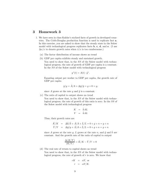
3 <strong>Homework</strong> 3<br />
1. We have seen in class Kaldor’s stylized facts of growth in developed countries.<br />
The Cobb-Douglas production function is used to replicate fact a.<br />
In this exercise, you are asked to show that the steady state in the Solow<br />
model with technological progress replicates facts b, c, d, ande. (I use<br />
∆x/x to denote growth rates when ˙x/x is too cumbersome.)<br />
(a) The factor distribution of income shows no trend<br />
(b) GDP per capita exhibits steady and sustained growth.<br />
You need to show that, in the SS of the Solow model with technological<br />
progress, the rate of growth of GDP per capita is a constant.<br />
In the SS of the Solow model with technological progress<br />
y ∗ (t) =A(t) · ˜y ∗ .<br />
Equating output per worker to GDP per capita, the growth rate of<br />
GDP per capita<br />
˙y/y = ˙ A/A + ∆˜y/˜y = g +0=g,<br />
since A grows at the rate g and ˜y is a constant.<br />
(c) The ratio of capital to output shows no trend<br />
You need to show that, in the SS of the Solow model with technological<br />
progress, the rate of growth of this ratio is zero. In the SS of<br />
the Solow model with technological progress<br />
Thus, their growth rates are<br />
K = ˜ kAL<br />
Y = ˜ kAL<br />
˙K/K = ∆ ˜ k/ ˜ k + ˙<br />
A/A + ˙ L/L =0+g + n = g + n<br />
˙Y/Y = ∆˜y/y + ˙ A/A + ˙ L/L =0+g + n = g + n<br />
since A grows at the rate g, L grows at the rate n, and ˜y and ˜ k are<br />
constant. And the growth rate of the ratio of capital to output<br />
∆ (K/Y )<br />
(K/Y ) = ˙ K/K − ˙ Y/Y =0<br />
(d) The real rate of return to capital shows no trend<br />
You need to show that, in the SS of the Solow model with technological<br />
progress, the rate of growth of r is zero. We know that<br />
rK = αY, or<br />
r = αY/K.<br />
9
Youjustshowinpartc. that Y/K is a constant and we know that<br />
α is a constant. Therefore<br />
˙r ˙α ∆ (K/L)<br />
= +<br />
r α (K/L) =0+0=0<br />
(e) Wages exhibit sustained growth<br />
You need to show that, in the SS of the Solow model with technological<br />
progress, the rate of growth of w is a constant. We know<br />
that<br />
wL = (1−α)Y, or<br />
w = (1−α)y. Youjustshowinpartb. that y grows at the rate g and we know<br />
that (1 − α) is constant. Therefore<br />
˙w ∆(1 − α) ˙y<br />
= + =0+g = g.<br />
w (1 − α) y<br />
2. (The answer from the textbook is enclosed. A printout for my answer is<br />
also enclosed: differences between the two answers are due to rounding<br />
errors)<br />
It is easier to start calculating the case in which A converges completely;<br />
i.e., Â =1. The third column in the Table calculates ˆs, the fifth calculates<br />
h = exp(0.1 ∗ u) andthesixthcalculatesˆ h, the 8th calculates d0 = d + g +<br />
n =0.075 + n and the 9th calculates ˆ d0. Column 10 then calculates<br />
µ 1/2<br />
ˆs<br />
ˆh<br />
ˆd0<br />
using columns 3, 6 and 9. To calculate the case in which the 1990 TFP<br />
ratios are maintained, we just need to multiply the previous answer by<br />
the 1990 TFP ratios (columns 10 and 12) to obtain column 13.<br />
The distance in this case is calculated following your method:<br />
ˆy ∗ − ˆy97<br />
ˆy ∗ .<br />
As you can see the countries are ranked by the rate of growth (or distance)<br />
in the first case 1 so Cameroon will grow the fastest and the US the slowest.<br />
In the second case, Argentina is predicted to grow at a rate below "normal"<br />
(that of the States) and the rank is as follows (from fastest to slowest):<br />
1) Cameroon, 2) Canada, 3) Thailand, 4) USA, 5) Argentina. (You were<br />
only asked which economy will be the fastest and which the slowest.)<br />
1 The answer in the textbook mixes cases a) and b)<br />
10
3 Empirical Applications of Neoclassical Growth Models<br />
Exercise 1. Where are these economies headed?<br />
From equation (3.9), we get<br />
ˆy ∗ =<br />
α <br />
ˆsK 1−α<br />
ˆh  =<br />
ˆx<br />
ˆsK<br />
<br />
(n + 0.075)<br />
α<br />
1−α<br />
e ψ(u−uU.S.) Â,<br />
where the (ˆ) is used to denote a variable relative to its U.S. value and x = n+g+d.<br />
The calculations below assume α = 1/3 and ψ = .10, as in the chapter.<br />
Applying this equation using the data provided in the exercise leads to the<br />
following results for the two cases: Case (a) maintains the 1990 TFP ratios, while<br />
case (b) has TFP levels equalized across countries. The Ratio column reports the<br />
ratio of these steady-state levels to the values in 1997.<br />
ˆy97 (a) ˆy ∗ Ratio (b) ˆy ∗ Ratio<br />
U.S.A. 1.000 1.000 1.000 1.000 1.000<br />
Canada 0.864 1.030 1.193 1.001 1.159<br />
Argentina 0.453 0.581 1.283 0.300 0.663<br />
Thailand 0.233 0.554 2.378 0.259 1.112<br />
Cameroon 0.048 0.273 5.696 0.064 1.334<br />
The country furthest from its steady state will grow fastest. (Notice that by<br />
furthest we mean in percentage terms). So in case (a), the countries are ranked by<br />
their rates of growth, with Cameroon predicted to grow the fastest and the United<br />
States predicted to grow the slowest. In case (b), Cameroon is still predicted to<br />
grow the fastest while Argentina is predicted to grow the slowest.<br />
Exercise 2. Policy reforms and growth.<br />
The first thing to compute in this problem is the approximate slope of the relationship<br />
in Figure 3.8. Eyeballing it, it appears that cutting output per worker in<br />
half relative to its steady-state value raises growth over a 37-year period by about 2<br />
percentage points. (Korea is about 6 percent growth, countries at the 1/2 level are<br />
about 4 percent, and countries in their steady state are about 2 percent).<br />
10
y97 s s-hat u h h-hat n d' d'-hat y* (A-hat=1) distance A90 y* (A-hat90) distance<br />
USA 1 0.204 1.000 11.9 3.287 1.000 0.01 0.085 1.000 1.000 0.000 1 1.000 0.000<br />
Canada 0.864 0.246 1.206 11.4 3.127 0.951 0.012 0.087 1.024 1.033 0.163 0.972 1.004 0.139<br />
Argentina 0.453 0.144 0.706 8.5 2.340 0.712 0.014 0.089 1.047 0.584 0.225 0.517 0.302 -0.499<br />
Thailand 0.233 0.213 1.044 6.1 1.840 0.560 0.015 0.09 1.059 0.556 0.581 0.468 0.260 0.105<br />
Cameroon 0.048 0.102 0.500 3.4 1.405 0.427 0.028 0.103 1.212 0.275 0.825 0.234 0.064 0.253
3. Unemployment and growth. Consider how unemployment would affect<br />
the Solow growth model. Suppose that output is produced according<br />
to the production function Y = K α [(1−u ∗ )L] 1−α ,whereu ∗ is the natural<br />
rate of unemployment. There is no technological progress. Assume again<br />
that the labour force equals population.<br />
(a) Express output per worker, y, as a function of capital per worker, k,<br />
and the natural rate of unemployment. Describe the steady state of<br />
this economy.<br />
Output per worker equals<br />
y = Y<br />
L = Kα (1 − u∗ ) 1−αL1−α =(1−u<br />
L<br />
∗ ) 1−α<br />
µ α<br />
K<br />
=(1−u<br />
L<br />
∗ ) 1−α k α .<br />
A decrease in the natural rate of unemployment increases output<br />
per worker y at all levels of capital per worker k since there is more<br />
output to divide about: the production function curves shifts up.<br />
(Remember that workers are everybody in the labour force, not only<br />
the employed ones.)<br />
Since output per worker increases at all levels of k, investmentincreases<br />
at all levels of k, other things being equal (the investment<br />
curves shifts up); therefore, the capital per worker in the steady state,<br />
k ∗ , depends on the natural rate of unemployment.<br />
(Analytically, the steady state condition is the same:<br />
substituting<br />
sy = d 0 k;<br />
s(1 − u ∗ ) 1−α k α = d 0 k<br />
and solving for k<br />
k ∗ ³<br />
s<br />
=<br />
d0 You were not required to do this part.)<br />
´ 1<br />
1−α<br />
(1 − u ∗ ).<br />
(b) Suppose that some change in government policy reduces the natural<br />
rate of unemployment. Describe how this change affects output both<br />
immediately and over time. Is the steady-state effect on output larger<br />
or smaller than the immediate effect? Explain (Your answer should<br />
include a graph).<br />
The immediate effect is the increase in output per worker y at the<br />
same level of capital per capita k ∗ 1 (the old steady state capital per<br />
capita), from y∗ 1 to y0 2 =(1−u∗ 2) 1−αk∗ 1. However, this immediate<br />
effect also increases savings from s · y∗ 1 to s · y0 2 >d0 · k∗ 1 , greater than<br />
depreciation; therefore, there exists net investment which will start<br />
the process of accumulating more capital and moving to a higher<br />
steady state; i.e., the eventual effect (steady state) includes the extra<br />
increase in output due to the consequent increase in capital.<br />
11
(Analytically, suppose that the natural rate of unemployment is u ∗ 1.In<br />
the steady state,<br />
´ 1<br />
1−α<br />
k ∗ 1 =<br />
³<br />
s<br />
d0 y ∗ 1 =<br />
³<br />
s<br />
d0 The first effect would be<br />
y = (1−u ∗ 2) 1−α<br />
∙ ³<br />
s<br />
d0 (1 − u ∗ 2) 1−α ³ s<br />
d0 (1 − u ∗ 1) and<br />
´ α<br />
1−α<br />
(1 − u ∗ ).<br />
but eventually output per capita equals<br />
y ∗ 2 =<br />
´ 1<br />
1−α<br />
(1 − u ∗ ¸α<br />
1) =<br />
´ α<br />
1−α<br />
(1 − u ∗ 1) α<br />
³<br />
s<br />
d0 ´ 1<br />
1−α<br />
(1 − u ∗ 2).<br />
Again you were not required to do this.)<br />
4. The answer is enclosed.<br />
12
From the Mankiw-Romer-Weil (1992) model, we have the production function:<br />
Divide both sides by AL to get<br />
Y = K α H β (AL) 1−α−β .<br />
y<br />
A =<br />
α β k h<br />
.<br />
A A<br />
Using the (˜) to denote the ratio of a variable to A, this equation can be rewritten as<br />
˜y = ˜ k α˜ h β .<br />
Now turn to the capital accumulation equation:<br />
˙K = sKY − dK.<br />
As usual, this equation can be written to describe the evolution of ˜ k as<br />
˙˜k = sK ˜y − (n + g + d) ˜ k.<br />
Similarly, we can obtain an equation describing the evolution of ˜ h as<br />
and<br />
˙˜h = sH ˜y − (n + g + d) ˜ h.<br />
In steady state, ˙˜ k = 0 and ˙˜ h = 0. Therefore,<br />
˜k =<br />
˜h =<br />
sK<br />
n + g + d ˜y,<br />
sH<br />
n + g + d ˜y.<br />
Substituting this relationship back into the production function,<br />
˜y = ˜ k α˜<br />
<br />
β sK<br />
h =<br />
n + g + d ˜y<br />
α <br />
sH<br />
n + g + d ˜y<br />
Solving this equation for ˜y yields the steady-state level<br />
˜y ∗ α <br />
sK<br />
sH<br />
=<br />
n + g + d n + g + d<br />
β<br />
.<br />
β 1<br />
1−α−β<br />
.<br />
14
Finally, we can write the equation in terms of output per worker as<br />
y ∗ α <br />
sK<br />
sH<br />
(t) =<br />
n + g + d n + g + d<br />
Compare this expression with equation (3.8),<br />
y ∗ <br />
sK<br />
(t) =<br />
n + g + d<br />
α<br />
1−α<br />
hA(t).<br />
β 1<br />
1−α−β<br />
A(t).<br />
In the special case β = 0, the solution of the Mankiw-Weil-Romer model is<br />
different from equation (3.8) only by a constant h. Notice the symmetry in the<br />
model between human capital and physical capital. In this model, human capital<br />
is accumulated by foregoing consumption, just like physical capital. In the model<br />
in the chapter, human capital is accumulated in a different fashion — by spending<br />
time instead of output.<br />
15


