Download
1 / 15
530 likes | 1.45k Views
Model ARIMA Box-Jenkins. Pertemuan 11. Metodologi Box-Jenkins:. . 1. Identifikasi model untuk sementara data lampau digunakan untuk mengidentifikasi model ARIMA yang sesuai. 2. Penaksiran parameter pada model sementara

E N D
Model ARIMA Box-Jenkins Pertemuan 11
Metodologi Box-Jenkins: 1. Identifikasi model untuk sementara data lampau digunakan untuk mengidentifikasi model ARIMA yang sesuai. 2. Penaksiran parameter pada model sementara data lampau digunakan untuk mengestimasi parameter dari model sementara. 3. Pemeriksaan diagnosa, apakah model memadai? berbagai diagnosa digunakan untuk memeriksa kecukupan model sementara. jika memenuhi, maka model bisa digunakan untuk meramalkan. Bila tidak, maka ditetapkan model sementara yang baru. 4. Meramalkan model sementara yang sudah sesuai dapat digunakan untuk meramalkan nilai yang akan datang.
Diagram Metodologi Box-Jenkins Stationary dannon- stationary ACF dan PACF 1. Identifikasi model sementara 2. Estimasi parameter Tdk Testing parameter Tingkat residu Distribusi Normal dari residual 3. Pemeriksaaan diagnosa [ apakah modelmemadai? ] Ya 4. Meramalkan Perhitungan peramalan
Pola umum data time series Nonseasonal Stationary models Nonseasonal Nonstationary models Intervention models Seasonal and Multiplicative models ACF dan PACF
Stationary dan Nonstationary data Time Series Stationer Nonstationer
Perbedaan pertama: Zt = Y2t – Y2t-1 Nonstationer Differences Stationer
Sample Autocorrelation Function (ACF) For the working series Z1, Z2, …, Zn :
1 1 0 8 8 Lag k 0 Lag k -1 -1 1 1 0 0 8 8 Lag k Lag k -1 -1 ACF for stationary time series dies down (exponential) cuts off no oscillation dies down (sinusoidal) dies down (exponential) oscillation
1 1 Lag k 0 0 8 -1 -1 Lag k 8 Dying down fairly quickly versus extremely slowly Dying down fairly quickly stationary time series (usually) Dying down extremely slowly nonstationary time series (usually)
Sample Partial Autocorrelation Function (PACF) For the working series Z1, Z2, …, Zn : Corr(Zt,Zt-k|Zt-1,…,Zt-k+1)
Calculation of PACF at lag 1, 2 and 3 The sample partial autocorelations at lag 1, 2 and 3 are:
MINITAB output of STATIONARY time series ACF PACF Dying down fairly quickly Cuts off after lag 2
MINITAB output of NONSTATIONARY time series ACF PACF Cuts off after lag 2 Dying down extremely slowly
Explanation of ACF … [MINITAB output] + + t/2 . se(rk) t/2 . se(rk)
General Theoretical ACF and PACF of ARIMA Models ModelACFPACF MA(q): moving average of order qCuts offDies downafter lag q AR(p): autoregressive of order pDies downCuts offafter lag p ARMA(p,q): mixed autoregressive-Dies downDies downmoving average of order (p,q) AR(p) or MA(q)Cuts offCuts offafter lag qafter lag p No order AR or MANo spikeNo spike(White Noise or Random process)