Quadrotor Real-Time Simulation: A Temporary Computational Complexity-Based Approach

Abstract

The interaction of digital systems with dynamic systems requires synchrony and the accomplishment of time constrains, so the simulation of physical processes needs an implementation by means of real-time systems (RTS). However, as it can be expected, every simulation and/or implementation might demand too many computational resources, surpassing the capacity of the processor used by computational systems. This is the reason for the need to perform a temporary computational complexity analysis based on the study of the behavior of the execution times of the implemented simulation. In this regard, the Real-Time Operating Systems (RTOS) feature time managing tools, which allow their precise measurement and the establishment of scheduling criteria in process execution. Therefore, this research proposes accomplishing a temporary computational complexity analysis of the real-time simulation by an embedded system (ES) of an unmanned aerial vehicle (UAV) propelled by four rotors. Derived from this analysis, formal definitions are elaborated and proposed, which establish a close relationship between the temporary computational complexity and typical real-time temporary constraints. To the best of the author’s knowledge, the definitions presented in this article have not been reported in the literature. Furthermore, to perform the temporary computational complexity analysis of the UAV, the mathematical modeling based on the Euler–Lagrange approach is presented in detail. Finally, simulations were performed using a real-time system implemented on the Embedded Computer System (ECS) Raspberry Pi 2 Model B+, in order to validate the suggested definitions.

1. Introduction

Nowadays, digital systems performing specific functions have been developed and innovated, in a way that, due to the constant technological progress, more precise sensors have been manufactured, as well as digital systems for a specific use, which are known as embedded systems (ES). There is a great influence of the ES in electronic systems, for example, in electrical household appliances, navigation systems, unmanned aerial vehicles (UAV), automobiles, communication networks, and electrical energy distribution networks, among others. Due to their system-on-chip (SoC) architecture, energy efficiency, low cost, and portability, embedded computers represent an alternative for the implementation of feedback control systems in robots, servomechanisms, and small aircrafts. In this sense, the interaction of ES with the physical world requires synchrony and the accomplishment of time constraints for its correct function; therefore, real-time study and analysis are required.

According to [1,2], a real-time system (RTS) is any system that actively interacts with an environment whose dynamics are known [3]. This interaction happens in a certain occurrence instant ${\mu }_k$ of the physical world. The system’s output will be related to its entry through a processing time intrinsic to the real-time system. In this context, an RTS must fulfill three main characteristics: (a) Direct interaction with a real-world process through devices, such as sensors, Analogic/Digital Converters (ADC), Digital/Analogic Converters DAC), and actuators, among others; (b) emission of results according to the established times; and (c) rendering of correct responses at all times.

It is important to underline that the emission of such correct responses can vary temporarily due to the processing or calculating capacity of the system in real time, as well as to the number of elementary operations required to obtain the result in the established times. According to the preceding, the specified time intervals must be tied to a deadline designated by the system dynamics, as well as the time criteria of the sampling proposed by Nyquist [4], Kotel’nikov [5], and others.

On the other hand, the computational complexity theory is used to study the necessary hardware resources to calculate the solution to a problem. For that, the analysis of the required time for the execution of an algorithm is taken as a baseline, as well as the number of computational resources (memory, processor, priority management, etc.) used to do the calculation [6,7].

A clear illustration of the utilization of dynamic systems, whose simulation requires a numerical and computational analysis, can be found in the robotics field, with unmanned aerial vehicles (UAVs) serving as a prime example of this article. Several research articles have been held referring to UAV’s modeling and simulation, such as [8,9,10,11,12,13,14,15,16,17,18,19,20]. An example is shown in [21], where an alternative to evaluating a UAV’s performance without a physical environment is presented by means of a Gazebo open code simulator and the Robot Operating System (ROS), which allows the simultaneous simulations of different aspects, such as flight dynamics, Inertial Measurement Unit (IMU) integrated sensor, external image sensors, and complex environments. In addition, the quadrotor dynamics model was parameterized by means of wind tunnel tests and validated by comparing simulated and real flight data. The applicability for complex UAV simulation systems is shown using Visual Simultaneous Localization and Mapping (V-SLAM) approaches based on Light Detection and Ranging (LIDAR), available as open code software.

Another example is presented in [22], where a quadrotor simulator named Flightmare is proposed, which is constituted by two main tools: a configurable rendered engine built on Unity and a flexible physics engine for dynamic simulation. Both components may work independently, allowing the simulator to be high speed: the rendered one reaches rates of up to 230 Hz. In comparison, the physical simulation reaches rates of up to 200 Hz on a laptop. The simulator has been implemented using a laptop with 12-core Intel(R) Core(TM) i7-8850H CPU at up to 2.60 GHz. This also includes a multimodal sensor, an Application Programming Interface (API) for reinforcement learning that simulates hundreds of quadrotors simultaneously, and a virtual reality helmet, allowing interaction in the simulated medium. Two tasks were undertaken to prove its usefulness: the control of the quadrotor using deep reinforcement learning and the planning of routes to avoid collisions in a complex 3D environment. Furthermore, the UAV in this study is modeled as a rigid body driven by four engines. Finally, the quadrotor’s dynamic model was used to design control algorithms in the real world.

In contrast, [23] provided a generalized flight dynamic model of a quadrotor based on a novel hybrid Blade Element Momentum (BEM) theory. It allowed testing and evaluation of novel control and guidance algorithms, in simple software or hardware-in-the-loop simulations, for precise and aggressive maneuvers with an adequate performance. The controller development reduced the need for iterative gain tuning through flight tests. The systematic validation of the model was done through experiments and flight tests performed on an instrumented quadrotor.

Moreover, in [24] a low-cost, multi-rate, real-time distributed computing platform for dynamic simulation, control implementation, data visualization, and communications was presented. This platform is suitable for rapid virtual testing of aircraft system dynamics and control, including mission/path planning, flight control, propulsion, and energy management, by leveraging the off-the-shelf design and testing tools. The development was built on heterogeneous computing hardware, including real-time multi-core processors (running Linux system and PX4-based flight simulation/control/visualization) and Field-Programmable Gate Arrays (FPGA—a reconfigurable, parallel computing device). The mathematical models were solved by a set of multi-rate computational solvers and executed on multiple hardware units with different simulation time steps (or rates), depending on the model’s time scale. The controllers were implemented on either real-time multi-core processors running the Linux operating system, FPGA computing modules, or remote hardware controllers. Finally, the main contributions of this article highlight the use of this platform and show the results of a flight simulation case involving difficult dynamics in an autonomous flight mission.

According to the research mentioned above, the numerical and computational complexity of a physical process analysis, modeling, and simulation implies rising importance, mainly when intended to achieve an implementation with real-time capabilities. Therefore, a study based on temporary computational complexity would dimension the hardware benefits of an embedded system used to perform the simulation of a specific process. In addition, this approach would provide an alternative way to establish the sampling period that can be used when real-time implementations are required without relying on fundamental characteristics, such as the dynamic system time constant (which is not defined trivially in non-linear multivariable systems), among others.

Therefore, one of the most relevant contributions of this research study is the presentation of a set of formal definitions and concepts that illustrate the relationship between the analysis of temporary computational complexity and the time constraints proper of the RTS. Derived from these definitions is established some conditions that the simulation of an algorithm must meet so that its performance is in real time.

To illustrate the proposed approach, a real-time simulation of a UAV’s dynamic model has been implemented in the ECS Raspberry Pi 2 Model B+. Notice that although the UAV’s dynamic model has already been reported in several manuscripts in the literature, its mathematical development based on the Euler–Lagrange approach is presented in detail in this paper. This implementation allows one to denote how definitions and conditions describe and determine the temporary computational complexity based on an analysis of the measured execution times of the real-time tasks when using different priorities.

Finally, through the application of the developed theory, an analysis for the determination of the real-time tasks (RTT) deadline (which is a fundamental time constraint of the RTS) is offered and presented using a computational complexity analysis. This fact highlights a close relationship between temporary computational complexity and real-time systems. This analysis allows for the selection and recommendation of sampling periods by sizing the computer system’s hardware features by applying the temporary computational complexity analysis. Such a methodology is also ideal for computer systems that demand a speedy response and/or do not fail in accomplishing the deadline associated with its execution: for example, while implementing a control strategy using an RTS.

This article is organized as follows: Section 2 deals with the dynamic model of a UAV aircraft composed of four rotors (referenced in the rest of the article as quadrotor). Section 3 presents the real-time simulation of the quadrotor performed in the ECS Raspberry Pi 2 model B+, so the real-time response analysis is also shown. Section 4 presents the definitions formulated for the temporary computational complexity analysis of the quadrotor simulation algorithm implemented in the ES. This same section also addresses the relationship between the real-time systems and the temporary computational complexity. Finally, the discussion of the results is provided in Section 5, and the conclusions are presented in Section 6.

2. Mathematical Modeling

The aerial experimentation vehicle (referred to in further sections as drone, quadrotor, or UAV) has four actuators. The potential motions of the UAV are specified by manipulating the actuators; such movements are: (a) movement along with the x-axis; (b) movement along with the y-axis; and (c) movement along with the z-axis. To achieve the mentioned movements (x, y, z), the quadrotor’s orientation must be manipulated, which is accomplished by modifying or changing the pitch angle $\theta$, roll angle $\varphi$, and the yaw axis $\psi$, defined with regards to the UAV’s orientation framework. Taking this into consideration, it is helpful to mathematically specify how the quadrotor’s orientation is represented. As it is shown in Figure 1, the quadrotor is subject to the frames of reference C and I. Accordingly, C represents the non-inertial frame of reference, that is, a coordinate axis whose center is the quadrotor’s mass center; whereas I represents the inertial frame of reference, which is subject to the land surface (ground or platform from where the drone starts its navigation).

The quadrotor’s dynamics are established by the performance of four motions: thrust, yaw, pitch, and roll, as seen in Figure 2. It is possible to modify the drone’s spatial location by generating these motions. The motions outlined above must be controlled simultaneously so the quadrotor follows certain trajectories provided by a flight plan [8].

The quadrotor’s translational positions $\left[x,y,z\right]$, in rectangular coordinates regarding the inertial framework I, are defined by vector $\xi$.

$$\xi ={\left[x,y,z\right]}^T\in {\mathbb{R}}^3.$$

(1)

The quadrotor’s angular positions $\left[\psi ,\theta ,\varphi ,\right]$ (quadrotor’s orientation) regarding the non-inertial framework C is denoted by vector $\mathbf{\eta }$ (also known as the Euler angles vector).

$$\mathbf{\eta }={\left[\psi ,\theta ,\varphi ,\right]}^T\in {\mathbb{R}}^3.$$

(2)

The quadrotor’s total rotation can be found using the following rotation composition matrix, in which, for simplicity, $sin=S$ and $cos=C$ have been used:

$$\begin{array}{c}{\mathbf{R}}_{\mathbf{I}}=\mathbf{R}(z,\psi )•\mathbf{R}(y,\theta )•\mathbf{R}(x,\varphi ),\\ \mathbf{R}\left(z,\psi \right)=\left[\begin{array}{ccc}cos\psi & -sin\psi & 0\\ sin\psi & cos\psi & 0\\ 0& 0& 1\end{array}\right],\\ \mathbf{R}\left(y,\theta \right)=\left[\begin{array}{ccc}cos\theta & 0& sin\theta \\ 0& 1& 0\\ -sin\theta & 0& cos\theta \end{array}\right],\\ \mathbf{R}\left(x,\varphi \right)=\left[\begin{array}{ccc}1& 0& 0\\ 0& cos\varphi & -sin\varphi \\ 0& sin\varphi & cos\varphi \end{array}\right],\\ {\mathbf{R}}_{\mathbf{I}}=\left[\begin{array}{ccc}C\psi C\theta & -S\psi C\varphi +C\psi S\theta S\varphi & S\psi S\varphi +C\psi S\theta C\varphi \\ S\psi C\theta & C\psi C\varphi +S\psi S\theta S\varphi & -C\psi S\varphi +S\psi S\theta C\varphi \\ -S\theta & C\theta S\varphi & C\theta C\varphi \end{array}\right].\end{array}$$

(3)

The rotation matrix referred to framework C is defined as:

$$\begin{array}{c}{\mathbf{R}}_{\mathbf{C}}={{\mathbf{R}}_{\mathbf{I}}}^T=\\ =\left[\begin{array}{ccc}C\psi C\theta & S\psi C\theta & -S\theta \\ -S\psi C\varphi +C\psi S\theta S\varphi & C\psi C\varphi +S\psi S\theta S\varphi & C\theta S\varphi \\ S\psi S\varphi +C\psi S\theta C\varphi & -C\psi S\varphi +S\psi S\theta C\varphi & C\theta C\varphi \end{array}\right].\end{array}$$

(4)

Therefore, taking into account the above expressions, it is possible to represent the quadrotor dynamics in terms of the generalized coordinate vector $\mathbf{q}$, which is defined as:

$$\mathbf{q}={\left[x,y,z,\psi ,\theta ,\varphi \right]}^T\in {\mathbb{R}}^6.$$

(5)

The Euler–Lagrange equation, which allows the quadrotor to describe kinetic and potential energy, is defined as:

$$\Gamma {}_{\mathbf{i}}=\frac{d}{dt}\left(\frac{\partial L}{\partial \dot{{\mathbf{q}}_{\mathbf{i}}}}\right)-\frac{\partial L}{\partial {\mathbf{q}}_{\mathbf{i}}},$$

(6)

where:

• L is the Lagrangian function.
• ${\mathbf{q}}_{\mathbf{i}}$ is the generalized coordinate vector.
• $\dot{{\mathbf{q}}_{\mathbf{i}}}$ is the time derivative regarding the generalized coordinate vector.
• $\Gamma$${}_{\mathbf{i}}$ is the set of concurring forces acting over the aircraft.

The Lagrangian function is defined according to the following expression:

$$L=T-V.$$

(7)

where:

• T is the total kinetic energy.
• V is the total potential energy.

To develop the quadrotor’s dynamic model, the translational and rotational dynamics are analyzed separately, as is shown in the following:

Translational dynamics is determined by the elements that constitute vector $\xi$ given by (1), and it is defined as:

$$T_{traslacional}=\frac{m}{2}{\dot{\xi }}^{\mathbf{T}}\dot{\xi },$$

(8)

where m is the quadrotor’s mass and $\dot{\xi }$ denotes the time derivative of vector $\xi$.

Potential energy is defined as:

$$V=mgz,$$

(9)

where:

• g is the gravity’s acceleration.
• z is the quadrotor’s height.

The Lagrangian function for translational dynamics is defined as:

$$L_{traslacional}=T_{traslacional}-V.$$

(10)

Substituting (8) and (9) in (10), it is obtained:

$$L_{traslacional}=\frac{m}{2}{\dot{\xi }}^{\mathbf{T}}\dot{\xi }-mgz.$$

(11)

According to the Euler–Lagrange formalism (6), it is obtained for translational dynamics:

$$F_{\xi }=\frac{d}{dt}\left(\frac{\partial L_{traslacional}}{\partial \dot{\xi }}\right)-\frac{\partial L_{traslacional}}{\partial \xi },$$

(12)

where:

• $F_{\xi }$ represents the generalized force acting in the drone’s translational dynamics.

Solving (12) term by term, the following equations are obtained:

$$\frac{\partial L_{traslacional}}{\partial \xi }=-mg{\mathbf{E}}_{\mathbf{z}},$$

(13)

$${\mathbf{E}}_{\mathbf{z}}=\left[\begin{array}{c}0\\ 0\\ 1\end{array}\right],$$

(14)

$$\frac{\partial L_{traslacional}}{\partial \dot{\xi }}=m\dot{\xi },$$

(15)

$$\frac{d}{dt}\left(\frac{\partial L_{traslacional}}{\partial \dot{\xi }}\right)=m\ddot{\xi }.$$

(16)

Expressions (13)–(16) according to (12) can be more broadly represented as:

$${\mathbf{F}}_{\xi }=m\ddot{\xi }+mg{\mathbf{E}}_{\mathbf{z}}.$$

(17)

The generalized force ${\mathbf{F}}_{\xi }$ is also expressed in terms of the rotation composition matrix ${\mathbf{R}}_{\mathbf{I}}$ as:

$${\mathbf{F}}_{\xi }={\mathbf{R}}_{\mathbf{I}}\widehat{\mathbf{F}}\in {\mathbb{R}}^{\mathbf{3}}.$$

(18)

From Expression (18), $\widehat{\mathbf{F}}$ represents a compound vector in each element for each one of the forces delivered to the quadrotor´s engines. Such a vector is defined as follows:

$$\widehat{\mathbf{F}}=\left[\begin{array}{c}0\\ 0\\ u\end{array}\right].$$

(19)

From (19), u is defined as shown below:

$$u=f_1+f_2+f_3+f_4=f_i,i=1,2,3,4.$$

(20)

where:

• $f_i$ represents the force generated by each one of the aircraft’s four engines.

The forces generated by each one of the engines incorporated into the quadrotor are defined as:

$$f_i=k_i{{\omega }_i}^2,i=1,2,3,4$$

(21)

where:

• $k_i>0$ is a proportionality constant.
• ${\omega }_i$ is the angular velocity of each engine.

Substituting (18) and (3) into (17), it is obtained:

$${\mathbf{R}}_{\mathbf{I}}\widehat{\mathbf{F}}=m\left[\begin{array}{c}\ddot{x}\\ \ddot{y}\\ \ddot{z}\end{array}\right]+mg\left[\begin{array}{c}0\\ 0\\ 1\end{array}\right].$$

(22)

Developing the previous expression:

$$\left[\begin{array}{ccc}C\psi C\theta & -S\psi C\varphi +C\psi S\theta S\varphi & S\psi S\varphi +C\psi S\theta C\varphi \\ S\psi C\theta & C\psi C\varphi +S\psi S\theta S\varphi & -C\psi S\varphi +S\psi S\theta C\varphi \\ -S\theta & C\theta S\varphi & C\theta C\varphi \end{array}\right]\left[\begin{array}{c}0\\ 0\\ u\end{array}\right]=\left[\begin{array}{c}m\ddot{x}\\ m\ddot{y}\\ m\ddot{z}+mg\end{array}\right].$$

(23)

Translational dynamics is obtained by developing (23), resulting in:

$$\begin{array}{c}\ddot{x}=\left(S\psi S\varphi +C\psi S\theta C\varphi \right)\frac{u}{m},\\ \ddot{y}=\left(-C\psi S\varphi +S\psi S\theta C\varphi \right)\frac{u}{m},\\ \ddot{z}=\left(C\theta C\varphi \right)\frac{u}{m}-g.\end{array}$$

(24)

To develop the rotational dynamics modeling, it is first established that the generalized velocities $\dot{\mathbf{\eta }}$ are related to the angular velocity vector ${\omega }_{\mathbf{c}}$ regarding the quadrotor’s coordinate axis, as shown in (25):

$$\dot{\mathbf{\eta }}={{\mathbf{W}}_{\mathbf{\eta }}}^{-1}{\omega }_{\mathbf{c}}.$$

(25)

The calculation of ${\mathbf{W}}_{\mathbf{\eta }}$ implicit in (25) is given by (for more information see Appendix A):

$${\mathbf{W}}_{\mathbf{\eta }}=\left[\begin{array}{ccc}-S\theta & 0& 1\\ S\varphi C\theta & C\varphi & 0\\ C\varphi C\theta & -S\varphi & 0\end{array}\right].$$

(26)

The matrix $\mathbb{J}=\mathbb{J}\left(\mathbf{\eta }\right)$, defined by (27), acts as an inertia matrix in the calculation of the rotational kinetic energy.

$$\mathbb{J}={{\mathbf{W}}_{\mathbf{\eta }}}^T\mathbf{I}{\mathbf{W}}_{\mathbf{\eta }}.$$

(27)

Assuming that the quadrotor’s structure is symmetrical, from (27), the matrix $\mathbf{I}$ is defined as:

$$\mathbf{I}=\left[\begin{array}{ccc}{I}_{xx}& 0& 0\\ 0& I_{yy}& 0\\ 0& 0& I_{zz}\end{array}\right].$$

(28)

Substituting (28) and (26) in (27), it is obtained:

$$\mathbb{J}=\left[\begin{array}{ccc}-S\theta & S\varphi C\theta & C\varphi C\theta \\ 0& C\varphi & -S\varphi \\ 1& 0& 0\end{array}\right]\left[\begin{array}{ccc}{I}_{xx}& 0& 0\\ 0& I_{yy}& 0\\ 0& 0& I_{zz}\end{array}\right]\left[\begin{array}{ccc}-S\theta & 0& 1\\ S\varphi C\theta & C\varphi & 0\\ C\varphi C\theta & -S\varphi & 0\end{array}\right].$$

(29)

According to the previous expressions, the rotational kinetic energy is defined as:

$$T_{rotacional}=\frac{1}{2}{\dot{\mathbf{\eta }}}^{\mathbf{T}}\mathbb{J}\dot{\mathbf{\eta }}.$$

(30)

The torque or moments of roll ${\tau }_{\varphi }$, pitch ${\tau }_{\theta }$, and yaw ${\tau }_{\psi }$ (also known as generalized moments) are defined by the following expression:

$${\mathbf{\tau }}_{\mathbf{\eta }}=\left[\begin{array}{c}{\tau }_{\psi }\\ {\tau }_{\theta }\\ {\tau }_{\varphi }\end{array}\right]=\left[\begin{array}{c}{\tau }_{m1}-{\tau }_{m2}+{\tau }_{m3}-{\tau }_{m4}\\ (f_1-f_3)l\\ (f_2-f_4)l\end{array}\right],$$

(31)

where:

• l is the distance between the engines and the quadrotor’s mass center.

The moment produced by each one of the quadrotor’s engines is defined as:

$${\tau }_{mi},i=1,2,3,4.$$

(32)

The moment of yaw is also defined as:

$${\tau }_{\psi }=\left(f_1+f_3\right)l-\left(f_2+f_4\right)l.$$

(33)

The Lagrangian function for rotational dynamics is defined as:

$$L_{rotacional}=\frac{1}{2}{\dot{\mathbf{\eta }}}^{\mathbf{T}}\mathbb{J}\dot{\mathbf{\eta }}.$$

(34)

Substituting (34) on the Euler–Lagrange formalism (6), it is obtained for rotational dynamics:

$${\mathbf{\tau }}_{\mathbf{\eta }}=\frac{d}{dt}\left(\frac{\partial L_{rotacional}}{\partial \dot{\mathbf{\eta }}}\right)-\frac{\partial L_{rotacional}}{\partial \mathbf{\eta }}.$$

(35)

The equations defined by (35) can also be expressed as:

$${\mathbf{\tau }}_{\mathbf{\eta }}=\frac{d}{dt}\left(\mathbb{J}\dot{\mathbf{\eta }}\right)-\frac{1}{2}\frac{\partial }{\partial \mathbf{\eta }}\left({\dot{\mathbf{\eta }}}^{\mathbf{T}}\mathbb{J}\dot{\mathbf{\eta }}\right).$$

(36)

Performing operations in (36), it is obtained:

$${\mathbf{\tau }}_{\mathbf{\eta }}=\mathbb{J}\ddot{\mathbf{\eta }}+\dot{\mathbb{J}}\dot{\mathbf{\eta }}-\frac{1}{2}\frac{\partial }{\partial \mathbf{\eta }}\left({\dot{\mathbf{\eta }}}^{\mathbf{T}}\mathbb{J}\dot{\mathbf{\eta }}\right).$$

(37)

From (37), the Coriolis vector $\mathbf{V}(\mathbf{\eta },\dot{\mathbf{\eta }})$ is defined as:

$$\mathbf{V}(\mathbf{\eta },\dot{\mathbf{\eta }})=\dot{\mathbb{J}}\dot{\mathbf{\eta }}-\frac{1}{2}\frac{\partial }{\partial \mathbf{\eta }}\left({\dot{\mathbf{\eta }}}^{\mathbf{T}}\mathbb{J}\dot{\mathbf{\eta }}\right).$$

(38)

The Coriolis matrix $\mathbf{C}\left(\mathbf{\eta },\dot{\mathbf{\eta }}\right)$ defines the centrifuge and gyroscopic effect typical of rotational dynamics. Such a matrix is obtained from (38) and it is expressed as:

$$\mathbf{V}\left(\mathbf{\eta },\dot{\mathbf{\eta }}\right)=\left[\dot{\mathbb{J}}-\frac{1}{2}\frac{\partial }{\partial \mathbf{\eta }}\left({\dot{\mathbf{\eta }}}^{\mathbf{T}}\mathbb{J}\right)\right]\dot{\mathbf{\eta }}=\mathbf{C}\left(\mathbf{\eta },\dot{\mathbf{\eta }}\right)\dot{\mathbf{\eta }}.$$

(39)

Considering Expressions (38) and (39), Equation (37) is also defined as:

$${\mathbf{\tau }}_{\mathbf{\eta }}=\mathbb{J}\ddot{\mathbf{\eta }}+\mathbf{V}(\mathbf{\eta },\dot{\mathbf{\eta }}),$$

(40)

$${\mathbf{\tau }}_{\mathbf{\eta }}=\mathbb{J}\ddot{\mathbf{\eta }}+\mathbf{C}\left(\mathbf{\eta },\dot{\mathbf{\eta }}\right)\dot{\mathbf{\eta }}.$$

(41)

The Coriolis matrix calculation possesses the general form of the following:

$$\mathbf{C}\left(\mathbf{\eta },\dot{\mathbf{\eta }}\right)=\left[\dot{\mathbb{J}}-\frac{1}{2}\frac{\partial }{\partial \mathbf{\eta }}\left({\dot{\mathbf{\eta }}}^{\mathbf{T}}\mathbb{J}\right)\right]=\left[\begin{array}{ccc}{C}_{11}& C_{12}& C_{13}\\ C_{21}& C_{22}& C_{23}\\ C_{31}& C_{32}& C_{33}\end{array}\right].$$

(42)

Appendix A of this article contains the calculation for the inertia $\mathbb{J}$ and the Coriolis matrix $\mathbf{C}\left(\mathbf{\eta },\dot{\mathbf{\eta }}\right)$. Finally, the quadrotor’s rotational dynamics can be represented by the following expression, which is obtained from (41):

$$\ddot{\mathbf{\eta }}={\mathbb{J}}^{-1}\left[{\mathbf{\tau }}_{\mathbf{\eta }}-\mathbf{C}\left(\mathbf{\eta },\dot{\mathbf{\eta }}\right)\dot{\mathbf{\eta }}\right].$$

(43)

The operation point is settled around the equilibrium point, in which the quadrotor is in a stationary state, to perform the reduced rotational dynamics modeling; that is, it is regarded that $(\psi =0,\theta =0,\varphi =0)$. The necessity to explore these reduced dynamics stems from the fact that the dynamics defined by (43) are not simple. It is essential to underline that the approach described above only works for flight trajectories with no abrupt transitions. Thus, the Euler angles will be small.

According to the preceding considerations, given the reduced rotational dynamics, it is proved that:

$$sin\psi \approx sin\theta \approx sin\varphi =0.$$

(44)

$$cos\psi \approx cos\theta \approx cos\varphi =1.$$

(45)

Substituting the small-angle considerations described by (44) and (45) into the defined rotational dynamics defined by (41), it is obtained:

$${\mathbf{\tau }}_{\mathbf{\eta }}=\overline{\mathbb{J}}\ddot{\mathbf{\eta }}+\overline{\mathbf{C}}\left(\mathbf{\eta },\dot{\mathbf{\eta }}\right)\dot{\mathbf{\eta }},$$

(46)

where:

$$\overline{\mathbb{J}}=\left[\begin{array}{ccc}{I}_{zz}& 0& 0\\ 0& I_{yy}& 0\\ 0& 0& I_{xx}\end{array}\right],$$

(47)

$$\overline{\mathit{C}}\left(\mathbf{\eta },\dot{\mathbf{\eta }}\right)=\left[\begin{array}{ccc}0& I_{yy}\dot{\varphi }-I_{zz}\dot{\varphi }& {-I}_{xx}\dot{\theta }\\ 0& 0& I_{xx}\dot{\psi }+I_{yy}\dot{\psi }-I_{zz}\dot{\psi }\\ 0& {-I}_{xx}\dot{\psi }-I_{yy}\dot{\psi }+I_{zz}\dot{\psi }& 0\end{array}\right].$$

(48)

Solving the matrix operations of Expression (46), it is obtained:

$$\left[\begin{array}{c}{\tau }_{\psi }\\ {\tau }_{\theta }\\ {\tau }_{\varphi }\end{array}\right]=\left[\begin{array}{c}{I}_{zz}\ddot{\psi }+\left(I_{yy}\dot{\varphi }-I_{zz}\dot{\varphi }{-I}_{xx}\dot{\varphi }\right)\dot{\theta }\\ I_{yy}\ddot{\theta }+(I_{xx}\dot{\psi }+I_{yy}\dot{\psi }-I_{zz}\dot{\psi })\dot{\varphi }\\ I_{xx}\ddot{\varphi }+(-I_{xx}\dot{\psi }-I_{yy}\dot{\psi }+I_{zz}\dot{\psi })\dot{\theta }\end{array}\right].$$

(49)

Solving and rewriting the implicit expressions in (49), the quadrotor’s reduced rotational dynamics are defined as:

$$\begin{array}{c}\ddot{\psi }=\frac{{\tau }_{\psi }}{I_{zz}}+\frac{(I_{xx}-I_{yy})\dot{\varphi }\dot{\theta }}{I_{zz}}+\dot{\varphi }\dot{\theta },\\ \ddot{\theta }=\frac{{\tau }_{\theta }}{I_{yy}}+\frac{(I_{zz}-I_{xx})\dot{\psi }\dot{\varphi }}{I_{yy}}-\dot{\psi }\dot{\varphi },\\ \ddot{\varphi }=\frac{{\tau }_{\varphi }}{I_{xx}}+\frac{(I_{yy}-I_{zz})\dot{\psi }\dot{\theta }}{I_{xx}}+\dot{\psi }\dot{\theta }.\end{array}$$

(50)

Finally, the aircraft’s non-linear dynamic model is defined by combining the translational dynamics (24) with the reduced rotational dynamics (50), resulting as follows:

$$\begin{array}{c}\ddot{x}=\left(S\psi S\varphi +C\psi S\theta C\varphi \right)\frac{u}{m},\\ \ddot{y}=\left(-C\psi S\varphi +S\psi S\theta C\varphi \right)\frac{u}{m},\\ \ddot{z}=\left(C\theta C\varphi \right)\frac{u}{m}-g,\\ \ddot{\psi }=\frac{{\tau }_{\psi }}{I_{zz}}+\frac{(I_{xx}-I_{yy})\dot{\varphi }\dot{\theta }}{I_{zz}}+\dot{\varphi }\dot{\theta },\\ \ddot{\theta }=\frac{{\tau }_{\theta }}{I_{yy}}+\frac{(I_{zz}-I_{xx})\dot{\psi }\dot{\varphi }}{I_{yy}}-\dot{\psi }\dot{\varphi },\\ \ddot{\varphi }=\frac{{\tau }_{\varphi }}{I_{xx}}+\frac{(I_{yy}-I_{zz})\dot{\psi }\dot{\theta }}{I_{xx}}+\dot{\psi }\dot{\theta },\end{array}$$

(51)

where the inputs to the model are defined by:

$$\begin{array}{c}u=f_1+f_2+f_3+f_4,\\ {\tau }_{\psi }=\left(f_1+f_3\right)l-\left(f_2+f_4\right)l,\\ {\tau }_{\theta }=(f_1-f_3)l,\\ {\tau }_{\varphi }=(f_2-f_4)l.\end{array}$$

(52)

3. Real-Time Simulation

Nowadays, real-time systems (RTS) play a primordial role in human existence because they are in nearly everything we use: cellphones, microwave ovens, washing machines, TV sets, etc. For example, an RTS is used in the accurate operation of power plants and telephone stations, so the reliability of these services is guaranteed. Currently, there is a misconception about real-time systems in which it is expected that when they engage with a process, they do so immediately. However, fast systems are frequently mistaken for RTS.

Furthermore, according to [1,2], an RTS is such a digital system that is tailored to the time constraints given by the system or dynamic process according to diverse sampling criteria. It is thus established that a fast system produces its output without considering or respecting the time constraints of the environment’s process with which it interacts. Then, for this class of systems, we may state that the time it takes for data to get to the digital system is unimportant; only the time it takes for the output to be produced is important.

An RTS can be integrated by a personal computer (PC) and a RTOS that fulfills the constraints imposed by the dynamic process. For this, RTOS such as QNX^®, Lynx^®, RT-Linux^®, Emlid RT^®, and so on, can be used. These operating systems can provide proper support because of their multitasking capacities, synchronization, and message transmission, among other real-time system properties. As a result, the real-time systems implemented in a digital computer interact with the physical environment by using reconditioned variables by means of sensors, ADC, DAC, actuators [25], etc., which process their requests by means of real-time tasks $\left(J_i\right)$ [26,27,28]. A real-time task is an executable job entity $J_i$, which is at least characterized by an arrival time and a time constraint [2,29]. It is formed by a set of instances $j_{i,k}$, such that $J_i=\left\{j_{i,k}\right\},i,k\in {\mathbb{Z}}^{+}$, where i represents the task index and k represents the instance index [2,30]. Accordingly, an instance $j_{i,k}$ is a job unit of a task $J_i$, and it is defined with the following five-time constraints [1,2]:

$$\left(l_{i,k},s_{i,k}{,c}_{i,k},{f_{i,k},d}_{i,k}|i,k\in {\mathbb{Z}}^{+}\right).$$

(53)

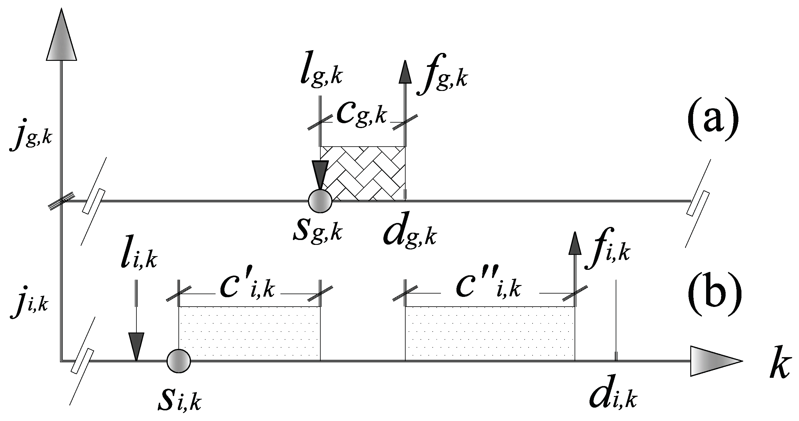
The definition of the time constraints associated with instances $j_{i,k}$ is the following:

Arrival time $l_{i,k}$: it is the time at the beginning of the process in which a task’s instance is placed in the ready queue. It is an absolute time in which the instance is queued until it is attended.

Start time $s_{i,k}$: it is the time when a task’s instance starts its execution.

Execution time $c_{i,k}$: it is the time when a real-time task’s instance performs its operations without considering its displacements in the processor.

Ending time $f_{i,k}$: it is the time when a task’s instance finishes its execution within interval k.

Deadline $d_{i,k}$: it is the maximum time when a local response has to be obtained from a real-time task’s instance without negatively altering the process dynamics.

The time constraints of a real-time task’s instance have the graphic interpretation that can be seen in Figure 3.

Note that the execution time of an instance is not always equal to the difference between the ending time and the start time; instead, it may change according to scheduling criteria established by an RTT scheduler. A general way of describing said execution times is illustrated in Figure 4. However, it is important to note that this research work is carried out in the context of analyzing the temporary computational complexity of an algorithm whose execution times have been determined without focusing on specific RTT scheduling criteria.

In context with that mentioned above, the quadrotor’s dynamic model defined by (51) and (52) has been programmed in the ECS Raspberry Pi^®. For this purpose, some functions from a self-development library have been programmed using C language and the RTOS Emlid RT^®. This RTOS provides real-time support and time and priorities management tools that could allow a running algorithm to meet the time constraints imposed by a physical process, obtain correct answers, and consequently, meet the deadline associated with the RTT [31,32].

In addition, some functions of the developed software library are (a) use of matrices and vectors, (b) dynamic memory management, (c) simulation of systems expressed in state space form, and (d) numerical integration procedures based on Euler’s method. Therefore, for a real-time simulation of the drone’s mathematical model, the parameters shown in

Table 1. Parameters used for the real-time simulation of the drone dynamic model.

Parameter	Parameter Value	Units
Quadrotor’s mass (m)	1.4	Kg
Engine mass	0.088	Kg
Arm length	1.0	m
Axis x inertia ($I_{xx}$)	0.0116	Kg m${}^2$
Axis y inertia ($I_{yy}$)	0.0116	Kg m${}^2$
Axis z inertia ($I_{zz}$)	0.0232	Kg m${}^2$

, have been used.

To perform the quadrotor’s real-time simulation, the model described by (51) and (52) is recast in terms of the generalized coordinates specified by (5), taking into account that (54) is an alternate representation of the drone’s dynamic model.

$$\begin{array}{c}\ddot{\mathbf{q}}={\left[\ddot{x},\ddot{y},\ddot{z},\ddot{\psi },\ddot{\theta },\ddot{\varphi }\right]}^T\in {\mathbb{R}}^6=\\ {\ddot{q}}_1=\ddot{x}=\left(S\psi S\varphi +C\psi S\theta C\varphi \right)\frac{u}{m},\\ {\ddot{q}}_2=\ddot{y}=\left(-C\psi S\varphi +S\psi S\theta C\varphi \right)\frac{u}{m},\\ {\ddot{q}}_3=\ddot{z}=\left(C\theta C\varphi \right)\frac{u}{m}-g,\\ {\ddot{q}}_4=\ddot{\psi }=\frac{{\tau }_{\psi }}{I_{zz}}+\frac{(I_{xx}-I_{yy})\dot{\varphi }\dot{\theta }}{I_{zz}}+\dot{\varphi }\dot{\theta },\\ {\ddot{q}}_5=\ddot{\theta }=\frac{{\tau }_{\theta }}{I_{yy}}+\frac{(I_{zz}-I_{xx})\dot{\psi }\dot{\varphi }}{I_{yy}}-\dot{\psi }\dot{\varphi },\\ {\ddot{q}}_6=\ddot{\varphi }=\frac{{\tau }_{\varphi }}{I_{xx}}+\frac{(I_{yy}-I_{zz})\dot{\psi }\dot{\theta }}{I_{xx}}+\dot{\psi }\dot{\theta }.\end{array}$$

(54)

The dynamic model simulation defined by (54), considering the entries defined by (52), has been performed by successively integrating $\ddot{\mathbf{q}}$ and $\dot{\mathbf{q}}$ according to what is established in (55) and (56).

$$\dot{\mathbf{q}}=\int \ddot{\mathbf{q}}dt.$$

(55)

$$\mathbf{q}=\int \dot{\mathbf{q}}dt.$$

(56)

Euler’s numerical method was used to obtain the approximate solution for Expressions (55) and (56), and a real-time task $J_1$ was programmed with a simulation time of $20s$, and an iteration rate of $△t=$ 25 ms was proposed, resulting in 800 real-time instances. The simulation results are depicted in the following figures:

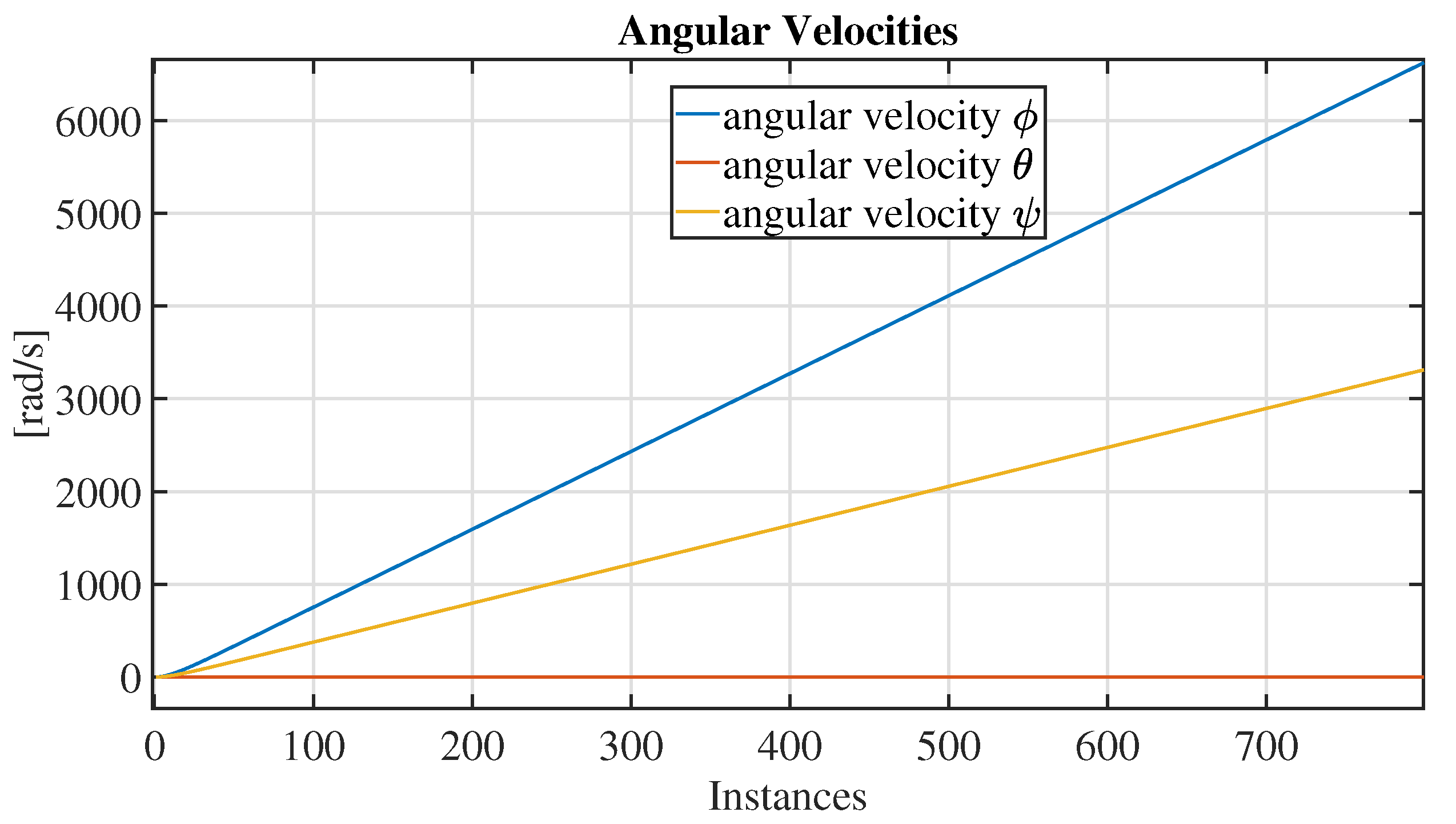
In Figure 5, the angular velocities $\varphi$, $\theta$, $\psi$ obtained in the quadrotor’s real-time simulation can be seen.

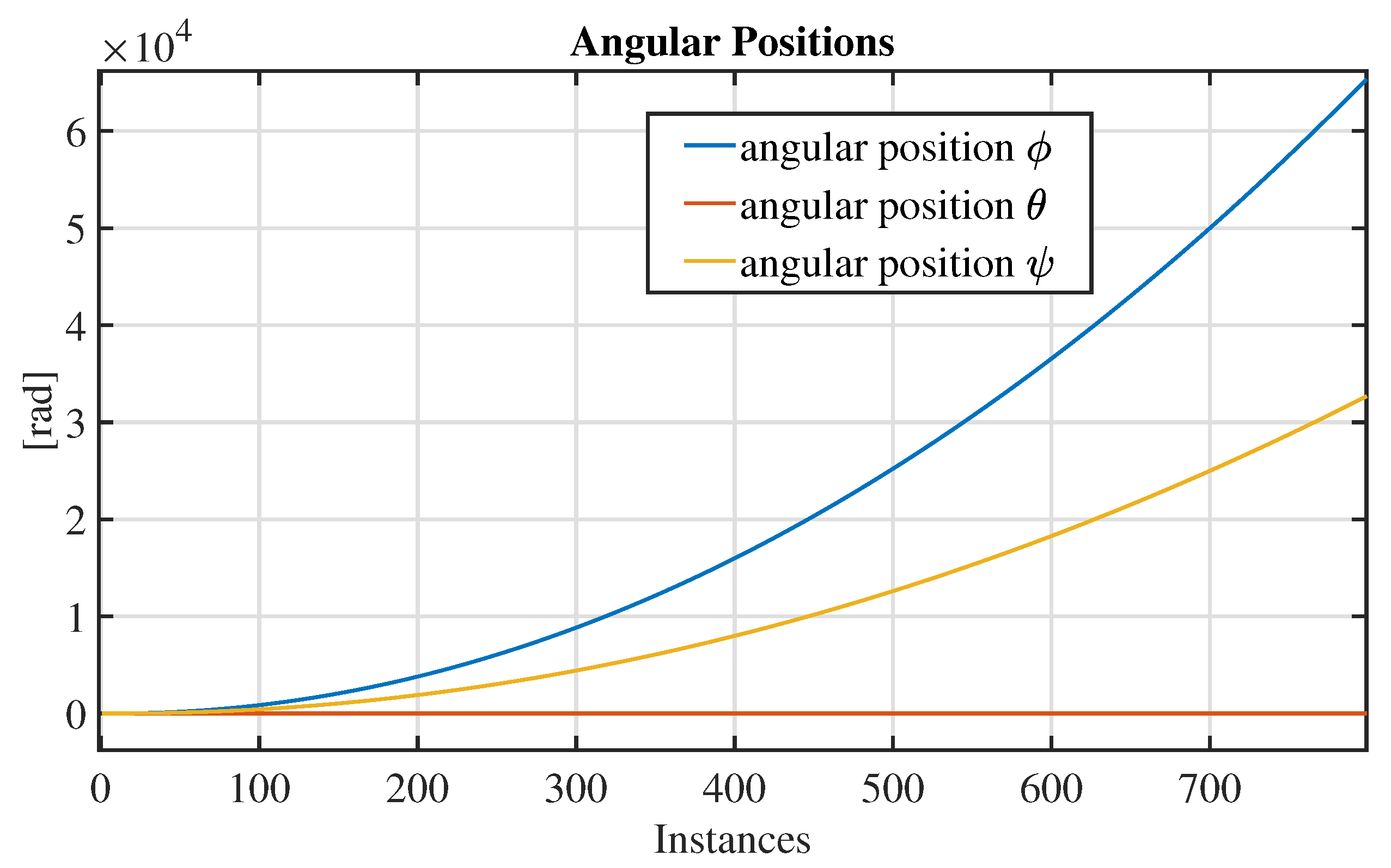
In Figure 6, the angular positions $\varphi$, $\theta$, $\psi$ obtained in the quadrotor’s real-time simulation are depicted.

In Figure 7, the translational velocities x, y obtained in the quadrotor’s real-time simulation are shown.

The translational velocities x, y, z acquired from the quadrotor’s real-time simulation are shown in Figure 8.

In Figure 9, the translational positions x, y obtained in the quadrotor’s real-time simulation can be seen.

The translational positions x, y, z obtained in the quadrotor’s real-time simulation are presented in Figure 10.

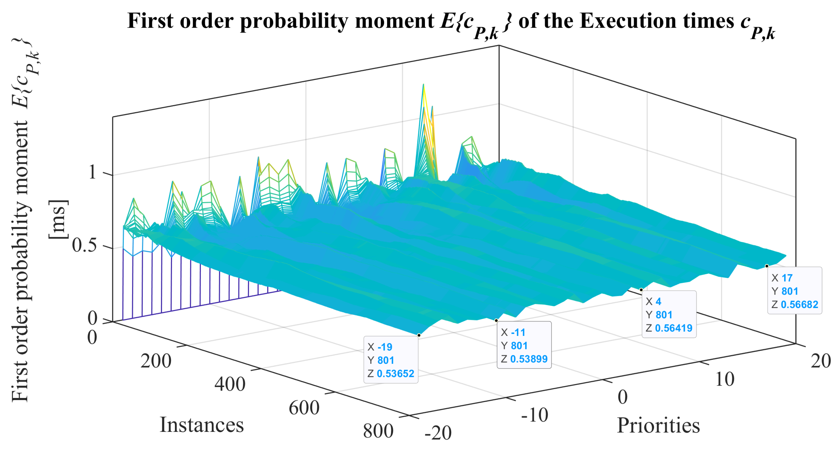
Once the quadrotor’s non-linear dynamic model was programmed, a simulation of this was performed in the embedded system, using distinct task execution priorities for that, which are comprehended in the interval from $-19$ and 19. Furthermore, the execution times of each instance were measured using the time management tools of the RTOS Emlid RT^®, yielding the execution times shown in Figure 11.

It is important to emphasize that in real-time operating systems, priority management indirectly impacts the RTT execution times because a real-time task that executes and has been configured with a higher priority is less likely to have its execution postponed (evicted in the processor) due to attending an RTT configured with a lower priority [33]. Consequently, those tasks configured with a high priority tend to define lower execution times than those with a lower priority. On the other hand, it is also important to note that according to [33,34,35], the use of RTT schedulers guarantees that those RTTs that are subject to eviction by the processor receive the necessary resources until completing their ending time (see Figure 4). However, note that the latter is outside of the purpose of this research work because the experimentation using different RTT schedulers has not been carried out; this is a proposal for future work. In this sense, and as it can be seen in Figure 12, where it is shown the first probability moment $E\left\{{\mathit{c}}_{\mathit{p},\mathit{k}}\right\}$ of the execution times of Figure 11 using a priority $p=-19$, it can be inferred that the highest possible priority is being used. Thus, the greatest amount of resources for the execution of the real-time task is being assigned. It is worth noting that using a priority $p=19$ implies that fewer resources are being given to the task’s execution.

As seen in Figure 11 and as it happens in any physical process, the behavior of execution times is random and varies over time. In this context, they also may be described as stochastic processes. The random behavior of such times is caused by various inherent characteristics in real-time operating systems such as pipeline, caching, process scheduling criteria, and priority management. It is important to note that although the behavior of the execution times is random, the deadlines determination based on a study of a temporary computational complexity of the algorithm could allow for the definition as to whether it has real-time performance or not. Therefore, this fact is part of the main motivation of the present research work, in which a study is proposed to evaluate the hardware benefits and their capability to meet specific RTT deadlines. This study is carried out through the elaboration of mathematical definitions aimed at justifying that the execution of the algorithm is performed by an RTS.

In real-time systems, the analysis and characterization of execution times $c_{i,k}$ and the deadline $d_{i,k}$ imposed for real-time task execution are critical for its good performance. Consequently, for each one of the real-time task’s instances $j_{1,k}$, the time constraint described by the following Expression (57) is considered.

$$d_{1,k}=△t=25\mathrm{ms}.$$

(57)

According to what has been stated above, it can be noted that every physical process in which the characterization of its time constraints is done could fulfills what is established by (58) and (59). In addition, if it is implemented in an embedded digital system, it has certain potentialities which allow it to be implemented in real-time using a real-time embedded system (RTES). In this sense, when a physical process is simulated using an algorithm programmed in an embedded digital computer, the analysis of its execution times $c_{i,k}$ and the fulfillment of the time constraint $d_{1,k}$ justify that the process simulation is working in real time. In this scenario, and according to the preceding reasons, the process simulation is appropriate to take place in real time. As a result, the following RTS classification is proposed.

Definition 1

(Hard Real-Time System HRTS).Any hard real-time system is the one in which the ending times $f_{i,k}$ are always in synchrony with the physical dynamics in all the evolution intervals. In these systems, it is mandatory that, for any instance, the following must be accomplished:

$$c_{i,k}<f_{i,k}\le d_{i,k}\forall c_{i,k},f_{i,k},d_{i,k}\in \mathbb{R}\wedge i,k\in {\mathbb{Z}}^{+}.$$

(58)

Definition 2

(Soft Real-Time System SRTS).Any soft real-time system is the one that, globally and in a sense of probability for its instances, accomplishes:

$$E\left\{c_{i,k}\right\}<d_{i,k}\forall c_{i,k},d_{i,k}\in \mathbb{R}\wedge i,k\in {\mathbb{Z}}^{+}.$$

(59)

Based on the real-time analysis previously stated, it can be summarized that the quadrotor’s simulation has been done by a hard real-time system, as the fulfillment of the deadline is performed according to what is established by (57). This implies that all the execution times $c_{i,k}$ (and their first probability moments) are less than the deadline imposed for the execution of the real-time task.

4. Temporary Computational Complexity

The study of the number of resources required by computational algorithms from the computer system is critical in their implementation. Despite technological advancements and the development of faster computers with more functions, their processing and storing capacity remains limited. Therefore, the amount of time and the number of memory sectors used by a computer system may describe a program in execution [36]. The description of this approach can be performed using a mathematical language in terms of functions and notations that may have universal validity and could represent a field of study. Thus, an algorithm’s temporary computational complexity determines the amount of time it takes to run. Likewise, the spatial computational complexity defines the amount of memory that an algorithm demands from a computing system to be executed.

Moreover, the temporary complexity is the amount of time it takes an algorithm to run in a digital system when its input data increases. However, regardless of how precise the time management tools of RTOS are, as is illustrated in Figure 11, execution times have a random evolution like any other physical process because they are influenced by additive noises, which also can be modeled as internal or external noises in the process [37]. Then, defining the behavior of an algorithm’s execution times without concern for the growth in its entry data or the computational system on which it is implemented is a topic of interest in scientific computing. Therefore, this research article proposes the representation of an algorithm’s temporary complexity by the function $T\left(n\right)$, where n denotes its entry data. According to this, the following definition is stated:

Definition 3

(Real-Time System’s Temporary Complexity TCC-RTS).The temporary complexity $T\left(n\right)$ of a real-time system is defined as a function that takes as its entry data the instances of an algorithm and maps them to the set of execution times $c_{i,k}$ measured, thus:

$$T\left(n\right):\left(n\right|n=j_{i,k})\to c_{i,k}.$$

(60)

According to the definition above, and considering that the temporary complexity is the amount of time that an algorithm requires to converge to a solution at the time that its entries increase, for any algorithm, these are essentially the evolution forms of $T\left(n\right)$ illustrated in Figure 13.

It is necessary to rebound, according to Figure 13, that any algorithm whose temporary complexity is of the linear $\left(T\right(n)=n)$, constant $\left(T\right(n)=1)$ or polynomial $(T\left(n\right)=n^x\forall x\ne n\wedge x\in \mathbb{R})$, is known as an algorithm with $\left(P\right)$ complexity or polynomial time.

In contrast to the previous algorithms, algorithms whose temporary complexity is of the non-polynomial $(T\left(n\right)=n^n)$ kind, also known as non-polynomial (NP) or of non-polynomial time, are hardly implemented using a real-time system, because those need too many resources from the computer system processor and are therefore deemed to potentially have an exponential complexity $(T\left(n\right)=2^n)$.

Therefore, knowing an algorithm’s temporary complexity entails understanding the behavior of its execution times $c_{i,k}$ and how these evolve over time, which itself represents a complex problem to solve. Moreover, as shown in Figure 11, the execution times of any algorithm implemented in an embedded computer by using an RTOS have a non-deterministic behavior. Consequently, and as a mathematical tool that provides an alternate solution to this problem, asymptotic notation is used to express the behavior of $T\left(n\right)$ as the number of entries n increases.

Asymptotic notation is named based on asymptotic functions, which appear to converge in one point when evaluated in specific threshold values; nonetheless, these never touch each other. As shown in Figure 14, asymptotic notation defines the function $g\left(n\right)$ as an upper or lower bound in describing deterministically the global behavior of the temporary complexity $T\left(n\right)$.

Therefore, the following definition of the function $g\left(n\right)$ is proposed:

Definition 4

(Function $\mathit{g}\left(\mathit{n}\right)$). Function $g\left(n\right)$ depicts the first probability moment of the random behavior of execution times $c_{i,k}$. Then, $g\left(n\right)$ can be represented as a function that tends to determinism and it is expressed as follows:

$$g\left(n\right)=\frac{1}{n}\sum _{n=1}^k{c}_{i,k}=E\left\{c_{i,k}\right\}.$$

(61)

The function described by (62) is proposed in this article as an alternative to (61), which defines a particular function that denotes execution times in a probabilistic approach. Then, function $g_D\left(n\right)$ is proposed, which is defined in terms of the constant $c_D$, execution times, and their initial probability moments, as follows:

$$g_D\left(n\right)=E\left\{c_{i,k}+c_{D}E\left\{c_{i,k}\right\}\right\}\forall c_D\in \mathbb{R}.$$

(62)

Given the definition of function $g_D\left(n\right)$ and the linearity properties of the first probability moment, the following mathematic manipulations can be proposed:

$$g_D\left(n\right)=E\left\{c_{i,k}\right\}+E\left\{c_{D}E\left\{c_{i,k}\right\}\right\},$$

(63)

$$g_D\left(n\right)=E\left\{c_{i,k}\right\}+c_{D}E\left\{E\left\{c_{i,k}\right\}\right\},$$

(64)

$$g_D\left(n\right)=E\left\{c_{i,k}\right\}+c_{D}E\left\{c_{i,k}\right\},$$

(65)

$$g_D\left(n\right)=\left(1+c_D\right)E\left\{c_{i,k}\right\},$$

(66)

$$g_D\left(n\right)=c\times g\left(n\right)\forall c\in \mathbb{R}|c>0\wedge c=1+c_D.$$

(67)

The Expressions (66) and (67) define the function $g_D\left(n\right)$ in terms of the function $g\left(n\right)$ and the constant c. Consequently, by means of the use of the condition denoted in the previous expressions, the function can either define an upper or a lower bound for function $T\left(n\right)$. According to Figure 14, the input to the algorithm in which an intersection between the functions $T\left(n\right)$ and $g\left(n\right)$ has occurred is called $n_0$.

Considering this analysis, the definition of function $g_{DCS}\left(n\right)$ is presented as follows:

Definition 5

(Function${\mathit{g}}_{\mathit{DCS}}\left(\mathbf{n}\right)$). Function $g_{DCS}\left(n\right)$ is every upper bound for every function $T\left(n\right)$ (and, consequently, for execution times $c_{i,k}$) and is defined by the following expression:

$$\begin{array}{c}{g}_{DCS}\left(n\right)=\underset{n\to \infty }{lim}\left\{g_D\left(n\right)\right\}=c\times g\left(n\right)|c\times g\left(n\right)\ge T\left(n\right)\\ \forall n>n_0|\parallel n_0\parallel \to 0\wedge \parallel n-n_0\parallel >\parallel n_0\parallel .\end{array}$$

(68)

Notice that every function $g_{DCS}\left(n\right)$ for which $n_0=0$ satisfies intrinsically the condition denoted by Expression (68), and, therefore, it can be established that its nature is to define an upper bound of $T\left(n\right)$ for all n.

The discrepancy $e_{GCS,T}\left(n\right)$ between any function $g_{DCS}\left(n\right)$ and $T\left(n\right)$ can be analyzed according to the following expression:

$$e_{GCS,T}\left(n\right)=\underset{n\to \infty }{lim}\left\{g_{DCS}\left(n\right)-T\left(n\right)\right\}.$$

(69)

It is important to underline that, according to the definitions stated above, and as long as the condition denoted by (68) is met, the magnitude of $e_{GCS,T}\left(n\right)$ can be decreased, as the magnitude of c decreases.

Similarly to Expression (68), the definition of function $g_{DCI}\left(n\right)$ is presented thus:

Definition 6

(Function${\mathit{g}}_{\mathit{DCI}}\left(\mathit{n}\right)$).Function $g_{DCI}\left(n\right)$ is every lower bound for every function $T\left(n\right)$ (and, consequently, for execution times $c_{i,k}$) and is defined by the following expression:

$$\begin{array}{c}{g}_{DCI}\left(n\right)=\underset{n\to \infty }{lim}\left\{g_D\left(n\right)\right\}=c\times g\left(n\right)|c\times g\left(n\right)\le T\left(n\right)\\ \forall n>n_0|\parallel n_0\parallel \to 0\wedge \parallel n-n_0\parallel >\parallel n_0\parallel .\end{array}$$

(70)

Based on the analysis of (68) and (70), it is feasible to determine that these may be used to dimension the hardware features of the embedded system where the physical process simulation is being performed. As a result, for each function $g_{DCS}\left(n\right)$, the smaller the magnitudes $\parallel c\parallel$ and $\parallel n_0\parallel$, the greater the processing power in the computing system used. In addition, notice that in real-time simulation, smaller sampling periods can be used, ensuring at all times and for future simulations the correct functioning in task execution. This allows for the avoidance of the overloading of the computing system by performing excessive operations that result in its blockage, which is derived from its memory overload, which is affected directly in the unfulfillment of the RTT’s deadline $d_{i,k}$.

Finally, using the definitions (60)–(62), (67), and (68), the temporary complexity of a real-time algorithm may be analyzed by the following definition:

Definition 7

(Function${\mathit{g}}_{\mathit{DD}}\left(\mathit{n}\right)$).Let us ${n=j}_{i,k}$ a set of instances of an algorithm implemented by a real-time system; the function $g_{DD}\left(n\right)$ is such that it maps its execution times to their deadlines, which is:

$$g_{DD}\left(n\right):c_{i,k}\to d_{i,k}|g_{DD}\left(n\right)=g_{DCS}\left(n\right).$$

(71)

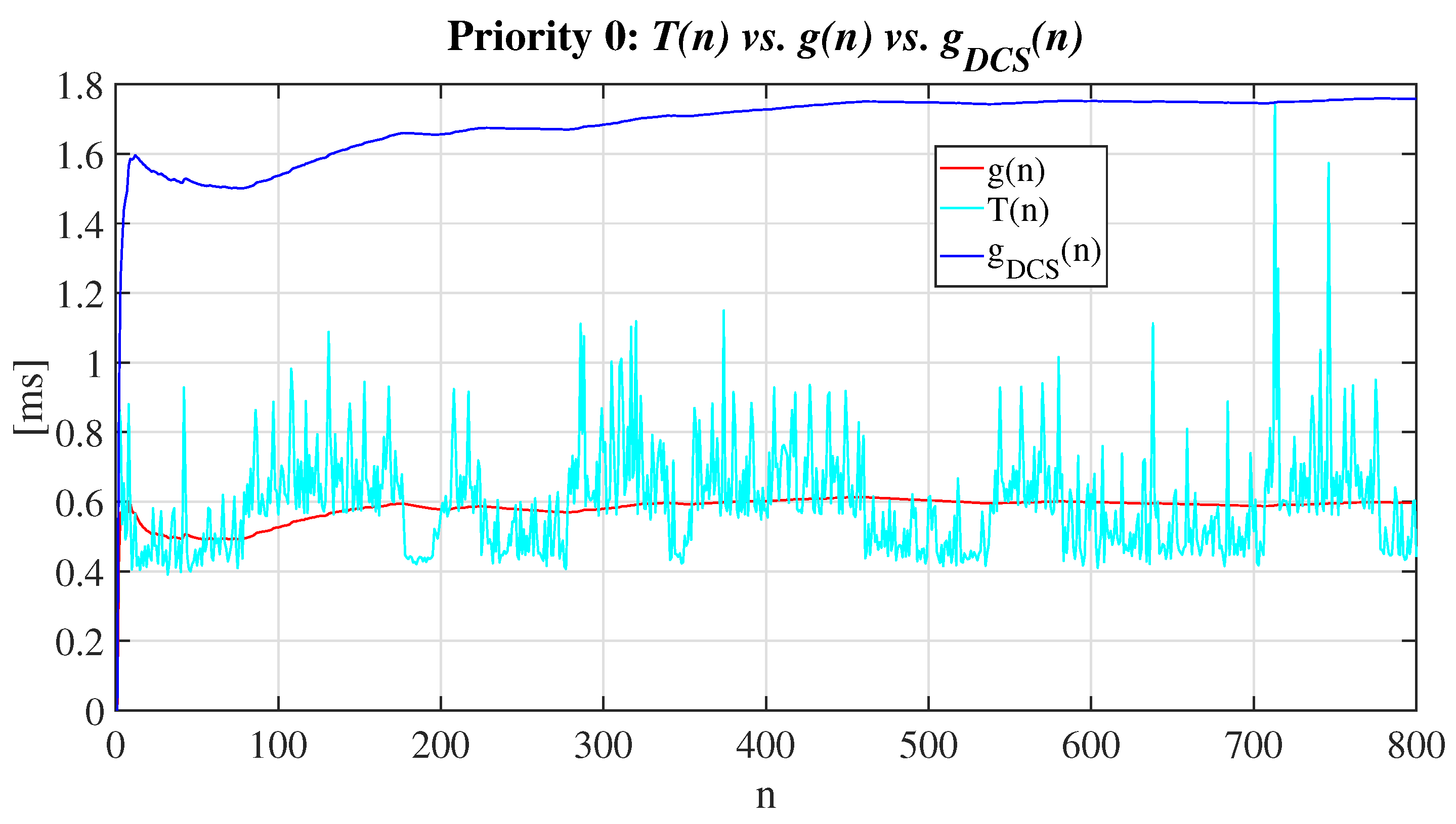
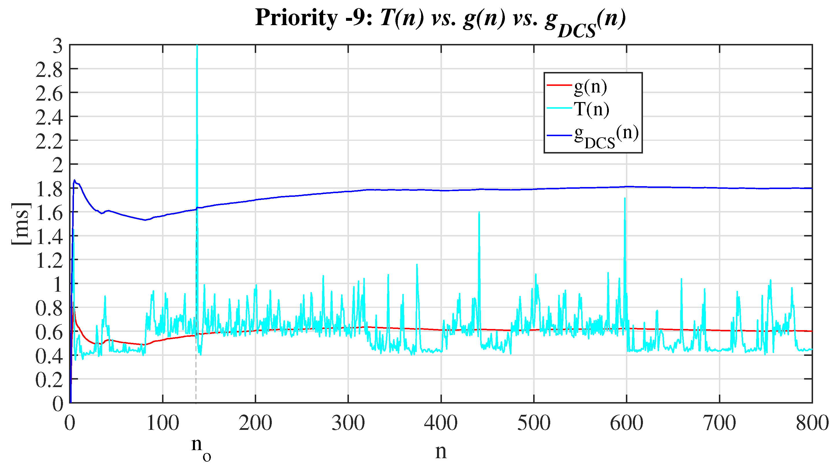
To validate the definitions proposed by this article, the results of the temporary computational complexity analysis of the algorithm performing the quadrotor’s real-time simulation (see Section 3) is presented. Consequently, the measured execution times of said algorithm are presented below. For that purpose, the priorities 19, 0, and $-19$ were taken into consideration; that is, in order to simulate the dynamic system by means of a real-time task, minimum, zero, and maximum priorities were used.

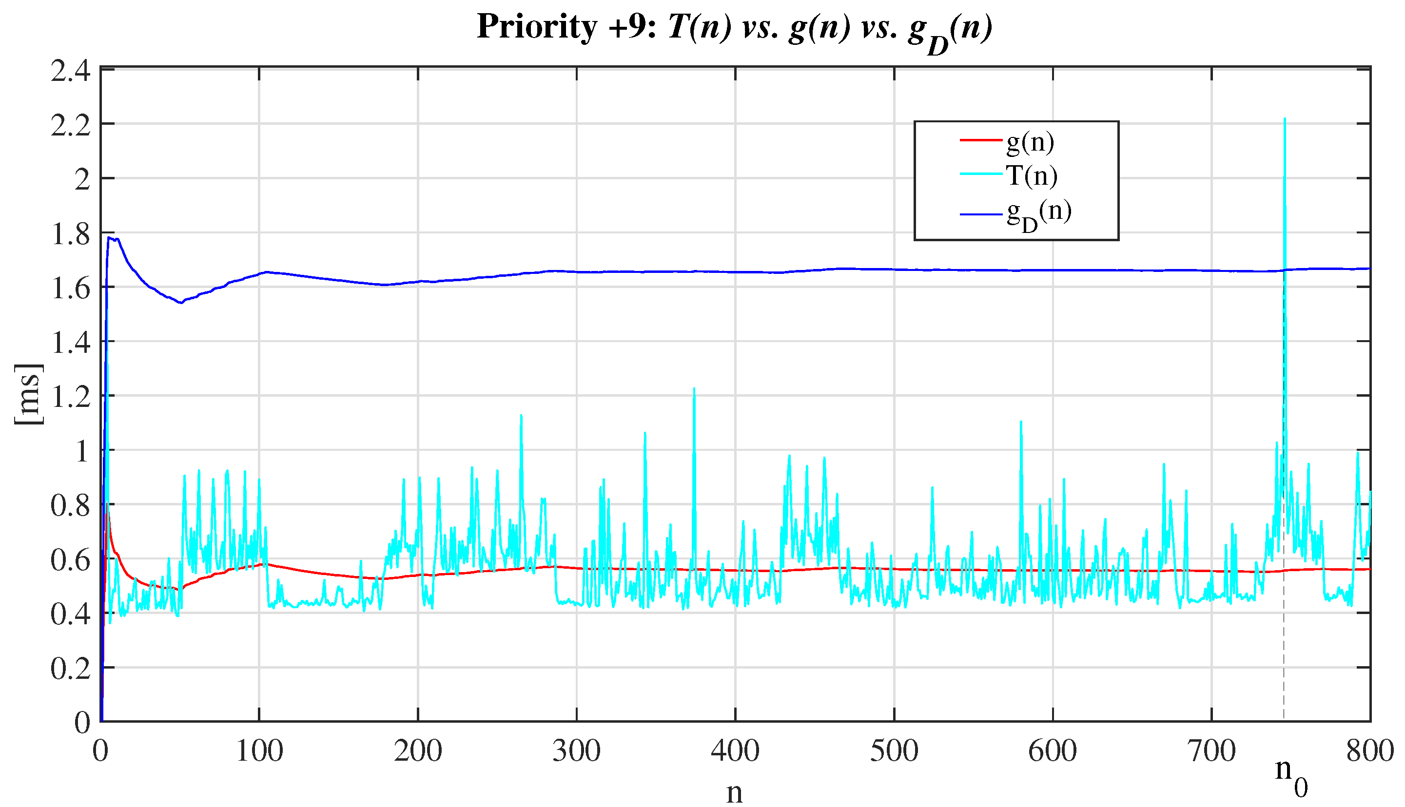
As shown in Figure 15, the use of the minimum priority in the execution of the algorithm that performs the quadrotor’s simulation has a direct influence on the measured execution times. When analyzing this response and comparing it to the responses of Figure 16, Figure 17, Figure 18 and Figure 19, it is possible to conclude that using this priority generates the maximum execution times in the embedded system; however, from these, it is possible to use the definition proposed by (68) to define the function $g_{DSC}\left(n\right)$, whose intrinsic nature is to represent an upper bound for function $T\left(n\right)$, because $n_0=0$.

Based on the analysis of $e_{GCS,T}\left(n\right)$ in Figure 15, and given the random behavior of $T\left(n\right)$, it can be concluded that this difference will tend to highlight the non-deterministic effect of the temporary computational complexity. Thus, for the analysis of $e_{GCS,T}\left(n\right)$, the following expression is proposed in addition to (69):

$$e_{GCS,G}\left(n\right)=\underset{n\to \infty }{lim}\left\{g_{DCS}\left(n\right)-g\left(n\right)\right\}.$$

(72)

The magnitude of the difference indicated in (72) (which can be seen in Figure 15) can be reduced when performing the quadrotor’s simulation using alternative priorities in the RTT’s execution. As a result, the experimentation shown in Figure 16, Figure 17, Figure 18 and Figure 19 denotes the possible dependency between the behavior of the execution times and the priorities. Regarding the results shown by Figure 16, which have used the priority $p=9$ and which have occurred in an intersection between $T\left(n\right)$ and $g_D\left(n\right)$ (domain value defined as $n_0$), the magnitude of $e_{GCS,G}\left(n\right)$ decreases effectively. However, function $g_D\left(n\right)$ does not fulfill the condition denoted by (68), as it is not accomplished for all domain n that $c\times g\left(n\right)\ge T\left(n\right)$. Additionally, the magnitude $\parallel n-n_0\parallel$ is not greater than $\parallel n_0\parallel$. Thus, function $g_D\left(n\right)$ does not acquire the character of upper bound, concluding that $g_D\left(n\right)\ne g_{DCS}\left(n\right)$.

As illustrated in Figure 17, the criterion set by (68) is met for all n; hence, the function $g_D\left(n\right)$ presented represents a upper bound for function $T\left(n\right)$. In consequence, it is proven that, given the intrinsic nature of $g_D\left(n\right)$, it is accomplished that: $g_D\left(n\right)=g_{DCS}\left(n\right)$. In this context, the fulfillment of the condition denoted by (68) prevails also for Figure 18 and Figure 19. Nevertheless, for the case that can be analyzed in Figure 18, function $g_D\left(n\right)$, does not fulfill $c\times g\left(n_0\right)\ge T\left(n\right)$; however, taking into account that condition (68) is accomplished for all $n>n_0$ and also $\parallel n-n_0\parallel >\parallel n_0\parallel$, it is possible to conclude (though not intrinsically) that: $g_D\left(n\right)=g_{DCS}\left(n\right)$.

It is worth noting, regarding Figure 19, that, similarly to what happens in Figure 15 and Figure 17, for all domain n, it is intrinsically fulfilled that $c\times g\left(n\right)\ge T\left(n\right)$. This, in consequence, for all three cases, we can prove that $g_D\left(n\right)=g_{DCS}\left(n\right)$ and that $n_0=0$. According to what was previously stated, and after analyzing the discrepancy $e_{GCS,G}\left(n\right)$ described by (72) and comparing such figures, it can be concluded that the lesser magnitude of such difference was obtained in the achieved experimentation using priorities $p=9$ and $p=-19$ in the RTT’s execution, resulting very similar in both cases (around 1.1 ms). The significant difference between these two cases is that only for this last priority the condition expressed by (68) is intrinsically fulfilled, because $n_0=0$, and this justifies that the optimal priority to perform the quadrotor’s real-time simulation in the used embedded system should be $p=-19$. Consequently, the selection of the algorithm execution priority in embedded systems that use a RTOS could be performed in the future using an optimal criterion in terms of decreasing the magnitude of $e_{GCS,G}\left(n\right)$, by fulfilling (preferably intrinsically) the condition (68).

Furthermore, using different priorities can influence the behavior of function $T\left(n\right)$, so that, for values close to $p=-19$, the amplitude of the function $g_{DCS}\left(n\right)$ associated with it can be minimized. As a result, if this process is performed fulfilling the condition expressed by (68), it is possible to use shorter sampling periods in the real-time simulation of dynamic systems, which is especially useful when these have very small time constants. The sampling period in a system’s real-time simulation is then represented by the temporary constraint described as deadline $d_{i,k}$. Then, as shown in this manuscript, one of the contributions presented is that the achievement of this temporary constraint can be studied in terms of the temporary computational complexity $T\left(n\right)$ and its interaction with the functions $g_D\left(n\right)$ and $g_{DCS}\left(n\right)$. In this regard, this research study provides as one of its contributions a technique for dimension the deadline $d_{i,k}$ in a real-time dynamic system simulation, whose application criterion is defined by (71).

One of the direct applications of the theory developed in this study might be the categorization of real-time systems based on the computational complexity analysis of algorithms implemented using an RTS. As a result of (71), and in addition to the definitions given by (58) and (59), in this article, the following categorization is proposed:

Definition 8

(Hard Real-Time System according to Temporary Computational Complexity Based Approach (HRTS-TCC)). All HRTS-TCC is HRTS whose temporary computational complexity should be intrinsically accomplished, that is to say, for all domain n, with the condition denoted by Expression (73). In these systems, it is imperative that $n_0=0$ when fulfilling such condition, this is:

$$\underset{n\to \infty }{lim}\left\{g_D\left(n\right)\right\}=c\times g\left(n\right)|c\times g\left(n\right)\ge T\left(n\right)|n_0=0.$$

(73)

Definition 9

(Soft Real-Time System according to Temporary Computational Complexity Based Approach SRTS-TCC). All SRTS-TCC is SRTS whose temporary computational complexity fulfills that denoted by (74). In these systems, it is imperative that $n_0\ne 0$ when fulfilling such condition, this is:

$$\begin{array}{c}\underset{n\to \infty }{lim}\left\{g_D\left(n\right)\right\}=c\times g\left(n\right)|c\times g\left(n\right)\ge T\left(n\right)\\ \forall n>n_0|\parallel n_0\parallel \to 0\wedge \parallel n-n_0\parallel >\parallel n_0\parallel .\end{array}$$

(74)

Notice that the behavior of function $T\left(n\right)$ when the number of entries of an algorithm increases can be defined in terms of function $g_D\left(n\right)$. In this context, its temporary computational complexity can be classified as it is established in

Table 2. Classification of the temporary computational complexity of an algorithm based on the behavior analysis of $T\left(n\right)$.

TCC	Relationship of $\mathit{T}\left(\mathit{n}\right)$ and ${\mathit{g}}_{\mathit{D}}\left(\mathit{n}\right)$	Execution Times
Exponential Complexity	$g_D\left(n\right)=2^n$	$c_{ei,k}$
Quadratic Complexity	$g_D\left(n\right)=n^2$	${c_{ci,k}|c_{ci,k}<c}_{ei,k}$
Linear Complexity	$g_D\left(n\right)=n$	${c_{li,k}|c_{li,k}<c}_{ci,k}$
Logarithmic Complexity	$g_D\left(n\right)=log\left(n\right)$	${c_{logi,k}|c_{logi,k}<c}_{li,k}$
Constant Complexity	$g_D\left(n\right)=1$	${c_{cti,k}|c_{cti,k}<c}_{logi,k}$

.

According to Table 2, each algorithm may be categorized based on an analysis of its temporary computational complexity. Then, those algorithms with a temporary complexity of the exponential kind, also known as non-polynomial time algorithms (NP) and whose function is $g_D\left(n\right)=2^n$ (implicit in Table 2), show that an increase in the entries n is translated into an increase in the exponential term. This implies that the growth rate of the function $T\left(n\right)$ increases, resulting in greater execution times $c_{ei,k}$ which lead to Table 2. The quadratic, linear, logarithmic, and constant complexity algorithms are known as polynomial-time algorithms (P). In this sense, they need substantially less processing time from the computer than NP-type algorithms when implemented. Therefore, one of the advantages of determining the temporary computational complexity of an algorithm is that it can predict how the time demand will rise when it is performed in the computer system. This is not straightforward because, as established in this article, execution times exhibit non-deterministic behavior. In addition to the aforesaid, it is necessary to know how they will behave (invariably from the computer system in which they are produced) when increasing the inputs to the algorithm; this indeed represents another aspect that complicates the computational complexity analysis.

Asymptotic notation is used to describe the temporary computational complexity; therefore, such notation is denoted by functions $T\left(n\right)$ and $g\left(n\right)$. As a result, the following definitions are provided below:

Definition 10

(Asymptotic Notation Big O).Temporary complexity $T\left(n\right)$ of an algorithm, has notation big O, that is to say, $T\left(n\right)\in O\left(g_D\left(n\right)\right)$ or $T\left(n\right)$ is of the order of $g_D\left(n\right)$, if constants $c\in \mathbb{R}$ and $n_0\in {\mathbb{Z}}^{+}$ exist, such that:

$$c\times g\left(n\right)\ge T\left(n\right)|c\times g\left(n\right)=g_D\left(n\right)=g_{DCS}\left(n\right).$$

(75)

Definition 11

(Asymptotic Notation Little o).Temporary complexity $T\left(n\right)$ of an algorithm, has notation little o, that is to say, $T\left(n\right)\in o\left(g_D\left(n\right)\right)$ or $T\left(n\right)$ is of the order of $g_D\left(n\right)$, if constants $c\in \mathbb{R}$ and $n_0\in {\mathbb{Z}}^{+}$ exist, such that:

$$c\times g\left(n\right)>T\left(n\right)|c\times g\left(n\right)=g_D\left(n\right)=g_{DCS}\left(n\right).$$

(76)

Definition 12

(Asymptotic Notation Big$\mathsf{\Omega }$). Temporary complexity $T\left(n\right)$ of an algorithm, has notation big Ω, that is to say $T\left(n\right)\in \Omega \left(g_D\left(n\right)\right)$ or $T\left(n\right)$ is of the order of $g_D\left(n\right)$, if constants $c\in \mathbb{R}$ and $n_0\in {\mathbb{Z}}^{+}$ exist, such that:

$$c\times g\left(n\right)\le T\left(n\right)|c\times g\left(n\right)=g_D\left(n\right)=g_{DCI}\left(n\right).$$

(77)

Definition 13

(Asymptotic Notation Little$\mathbf{\omega }$).Temporary complexity $T\left(n\right)$ of an algorithm, has notation little ω, that is to say, $T\left(n\right)\in \omega \left(g_D\left(n\right)\right)$ or $T\left(n\right)$ is of the order of $g_D\left(n\right)$, if constants $c\in \mathbb{R}$ and $n_0\in {\mathbb{Z}}^{+}$ exist, such that:

$$c\times g\left(n\right)<T\left(n\right)|c\times g\left(n\right)=g_D\left(n\right)=g_{DCI}\left(n\right).$$

(78)

Definition 14

(Asymptotic Notation Big$\mathsf{\Theta }$).Temporary complexity $T\left(n\right)$ of an algorithm, has notation big Θ, that is to say, $T\left(n\right)\in \mathsf{\Theta }\left(g_D\left(n\right)\right)$ or $T\left(n\right)$ is of the order of $g_{DS}\left(n\right)$ and of $g_{DI}\left(n\right)$, if constants $c_s,c_i\in \mathbb{R}$ and $n_{0s}$,$n_{0i}\in {\mathbb{Z}}^{+}$ exist, such that:

$$\begin{array}{c}{c}_s\times g_{DS}\left(n\right)\ge T\left(n\right)\ge c_i\times g_{DI}\left(n\right)\\ {|c}_s\times g_{DS}\left(n\right)=g_{DCS}\left(n\right)\wedge c_i\times g_{DI}\left(n\right)=g_{DCI}\left(n\right).\end{array}$$

(79)

According to the above definitions, the quadrotor’s temporary computational complexity may be described in terms of functions $g_D\left(n\right)$, as shown in Figure 15, Figure 16, Figure 17, Figure 18 and Figure 19. That is, functions $g_D\left(n\right)$ can be considered (taking into account Expressions (68) and (70)) as upper or lower bounds of functions $T\left(n\right)$. Then, as shown only in Figure 15 and Figure 17, Figure 18 and Figure 19 and by the accomplishment of the Expression (68), it can be concluded that functions $g_D\left(n\right)$ represent upper bounds for functions $T\left(n\right)$; this fact can confirm the Expression (71). In this context, as shown in the images, when n approaches infinity, the function $g_D\left(n\right)$ converges to a value (about $1.7milliseconds$), and this value may be stated according to what is established by (80).

$$\underset{n\to \infty }{lim}\left\{g_D\left(n\right)\right\}=0.0017\mathrm{s}.$$

(80)

An alternative way for Expression (80) to define the convergence value of the function $g_D\left(n\right)$, is as it is established by the following expression:

$$\underset{n\to \infty }{lim}\left\{g_D\left(n\right)\right\}=c_{D1}\underset{n\to \infty }{lim}\left\{g_{D1}\left(n\right)\right\}=0.0017\mathrm{s}.$$

(81)

It is important to note that, in (81), it is considered that the constant $c_{D1}=0.0017\in \mathbb{R}$ exists, and that function $g_{D1}\left(n\right)$ has the definition that can be observed in (82).

$$g_{D1}\left(n\right)=\left\{\begin{array}{c}1\forall n\ge 0\\ 0\forall n<0\end{array}\right.$$

(82)

Notice that, if, given the computational complexity of an algorithm $T\left(n\right)$, it is accomplished for all n that $c_{D1}\times g_{D1}\left(n\right)\ge g_D\left(n\right)$, in such a way that $g_D\left(n\right)$ is a upper bound for such $T\left(n\right)$. This implies that the condition denoted by (68) is fulfilled, and consequently $g_D\left(n\right)=g_{DCS}\left(n\right)$. In addition, by transitivity, it will be accomplish Expression (83), such that:

$$c_{D1}\times g_{D1}\left(n\right)\ge T\left(n\right)|c_{D1}\times g_{D1}\left(n\right)=g_{DCS}\left(n\right).$$

(83)

According to the behavior of functions $g_{DCS}\left(n\right)$, which can be seen in Figure 15 and Figure 17, Figure 18 and Figure 19, and to the definition of function $g_{D1}\left(n\right)$ given by (82) and Table 2, it can be summarized that the real-time simulation of the quadrotor’s dynamics presented in this article has a constant temporary computational complexity. Moreover, based on the analysis of (75) and (80)–(83), it is also established that complexity $T\left(n\right)$ of the real-time simulations reported in this article can be described by the asymptotic notation: big O.

5. Discussion

As it has been analyzed previously in this article, the computational complexity is a mathematical tool that permits the determination of, a priori, what the demand of resources will be, whether in time or space, of an algorithm whose entries increase when executed on a computer system. In this context, such analysis can be applied to any algorithm, whether it is implemented by means of a real-time system or not. Then, when an algorithm is implemented in a digital computer to simulate a dynamic system or physical process, this can or cannot accomplish the time constraints imposed by the process of the system which simulates the one with which it interacts. The fulfillment of this condition is one of the characteristics of real-time systems. The correct performance of those depends not only on the logical result that the computer retrieves but also on the time in which such a result is produced. For the RTS, they must respond to external events during their evolution, and results must be sent regularly, always meeting the deadlines set to the programmed real-time tasks. To achieve this goal, execution times (internal time) in the RTS must be measured precisely and on the same scale as environmental time (external time). When an RTS is implemented using RTOS, a real-time clock is used, as well as other tools, such as timers, concurrent programming, and priority management.

In contrast with the definition of RTS, an online system, whether rapid or instantaneous, produces its output without considering nor accomplishing the time constraints of the environment with which it interacts. For this kind of system, the time in which the data arrive at the digital system is not important but only the speed with which the output is produced. In other words, the speed in giving the response within a time interval whose measurement is better when smaller is the only important factor. That is, for this system, the cost of generating such a response, the accomplishing time constraints (deadlines), or the synchrony and periodicity do not matter, which are mandatory aspects in any RTS.

Considering the facts stated above, and according to the approach proposed in this article, an algorithm that interacts with or simulates a physical process in real time has a different kind of temporary computational complexity in comparison to one which is not implemented in real time. Therefore, the simulation of the model of a quadrotor achieved by means of an online system, (or off-line in the worst-case scenario) which depends on the number of iterations, and then, considering them as its entries, it would clearly have a linear kind of temporary computational complexity. Taking into account the previous analysis, it is evident that functions $T\left(n\right)$ seen in Figure 15, Figure 16, Figure 17, Figure 18 and Figure 19 have a complexity of the constant kind. This fact also justifies that the quadrotor (also known as drone) real-time simulation presented in this article has a temporary computational complexity of the constant kind and can be described using asymptotic notation big O. Regarding the functions $g_{DCS}\left(n\right)$ defined by (68), and which are observed in the previously mentioned figures, it can be assumed that the fact of using priorities close to $-19$ in the quadrotor’s real-time simulation modifies the discrepancy $e_{GCS,G}\left(n\right)$. This fact denotes a certain tendency to decrease it, and consequently, it could be interpreted that there is a strongly bounded dependency between c and p, in such a way that any modification of the value of p would imply a modification of the value of c. This interpretation is mistaken, as in this manuscript a constant value of c has been used in the definition of function $g_{DCS}\left(n\right)$. According to this, the most valid interpretation lies in the fact that, modifying the priority in a RTT’s execution, the discrepancy $e_{GCS,G}\left(n\right)$ is modified because the processor increases or decreases the number of task displacements according to the priority chosen and a scheduling criteria. Thus, when using a priority $p=-19$, the processor assigns the maximum quantity of hardware resources to the execution of the task in progress, reducing then the possibility of displacement by the necessity to attend any process requiring attention. This generates smaller execution times $c_{i,k}$, and consequently, the function $T\left(n\right)$ which converges to smaller values is defined, these being delimited by the function $g_{DCS}\left(n\right)$, which achieves convergence also to smaller values.

According to the definition of function $g\left(n\right)$ denoted by (61), and on which the analysis presented in this article is based, it is possible to assume that it is somewhat contradictory that the computing of this, when n is increased, will have, naturally, a temporary computational complexity of the linear kind. This fact represents an incongruency with the conclusion, in which the temporary complexity of the algorithm performing the real-time simulation is of the constant kind. However, it is important to highlight that, as it is shown in Appendix B of this article, function $g\left(n\right)$ can be expressed recursively and iteratively, which allows such function to be calculated in each instance of the real-time task that the quadrotor’s simulation performs. Finally, it is important to mention that the recursive expression of function $g\left(n\right)$ allows its easy implementation in any embedded system.

6. Conclusions

RTS are systems that, when interacting with a physical process, must accomplish at all times with certain temporary constraints. If these temporary constraints are not met, there is the possibility of the occurrence of a failure and/or collapse when real-time implementations of these physical processes are performed in embedded systems. Therefore, this research article proposes a set of formal definitions, such as; Real-Time System’s Temporary Complexity TCC-RTS, Hard Real-Time System with a Temporary Computational Complexity based Approach HRTS-TCC, Soft Real-Time System with a Temporary Computational Complexity based Approach SRTS-TCC, Asymptotic Notations, among others. These definitions contribute to the theory that allows the analysis of the temporary computational complexity of iterative algorithms programmed in embedded systems by means of RTS. Moreover, these definitions denote and establish a close relationship that can exist between the time constraints common to all RTS and the temporary computational complexity of the simulation and/or implementation of dynamic systems in embedded systems by proposing the use of different execution priorities. Therefore, one of the proposals of this research article allows for quantifying the hardware features and determining the conditions to accomplish the deadline of the RTT’s instances. To validate the definitions formulated in this manuscript, the detailed modeling of a quadrotor (UAV) according to the Euler–Lagrange approach was presented, where the simulation, implementation, and experimentation were carried out by means of an RTS implemented in the ECS Raspberry Pi 2 Model B+. This analysis of the real-time implementation allowed us to validate the characterization of the execution times of the implemented algorithm (UAV simulation) and also allowed us to present and analyze its temporary computational complexity through the definitions elaborated in this paper. This analysis also made it possible to determine the deadline of the real-time task, without analyzing the convergence rate of the dynamic system (quadrotor model). Therefore, this fact allows for the determination of the sampling periods that can be used by making a balance between the hardware features of the embedded computer system (Raspberry Pi), where the algorithm is implemented and its temporary computational complexity is found.

On the other hand, it is possible to highlight that by applying the developed theory in this manuscript, it would be possible to improve the performance of the autonomous flight algorithms in unmanned aerial vehicles. All this since it has been detected in the literature that tests in the studied UAVs still imply the risk of damage and/or failure due to the absence of implementation of their flight algorithms by means of an RTS, in which the deadline to be used is determined by an analysis of its temporary computational complexity. That is to say, the lack of analysis of the time constraints associated with the RTS can provoke the unfulfillment of the deadline of a specific task, in this way generating delays that impact negatively the stability of closed-loop control systems. This is the particular case of the implementation of the autonomous flight systems in UAVs.