Determinants of the Cost of Financial Intermediation: Evidence from Emerging Economies

Abstract

This study examines the determinants of financial intermediation costs of banks in ten Emerging Economies (EEs) in the period 2000–2018 using panel data of 1335 banks. Empirically, this study applies the single-stage dealership model and its extensions by introducing new bank and country-level variables. We find robust evidence that investment in government securities and market openness positively affect bank intermediation costs while the trilemma index negatively affects them. During the world financial crisis, bank intermediation costs increased. Moreover, we observe that cost inefficiency, credit risk, and regulatory regime are the crucial drivers of bank intermediation costs. We draw important implications for scholars and policymakers.

1. Introduction

A banking intermediary is a process of collecting surplus money from savers (those who have excess funds) and transferring it to borrowers (those who need funds) and thus plays a crucial role in economic development (Rahman et al. 2021). The banking industry contributes to the growth of several countries, of which emerging economies are no exception. As surveyed by (Zheng et al. 2017), efficiency in financial intermediation fosters economic growth. In addition to economic progress, tolerating bank margins also ensure social welfare. Thus, how much should the bank margin and its determinants be? It is an open empirical question that deserves special attention. Considerably too low and too high net interest margin is a persistent problem as this is the financial sector’s most important factor, such as the difference between lending interest rates and borrowing interest rates of the banks’ total earning assets. High-interest margin edge the financial intermediaries’ ability to contribute to growth and development, whereas the low return on deposits reduces the savings pattern of potential depositors and lessens the finance for future borrowers, subsequently deteriorating the possible investment flow and economic progress (Barajas et al. 1999). Similarly, Brock and Suarez (2000) argued that higher interest margins, on the one hand, could contribute to bank capitalization by transferring the profit earned to the capital base. On the other hand, higher interest margins are generally an indicator of banking sector inefficiency, and thus it would adversely affect domestic real savings and investment.

Meanwhile, the higher net interest margins induce the frictions of service cost and asymmetric information. Therefore, its impact is likely to be more severe in emerging economies. There are fewer chances of regulatory arbitrage by financial innovation in underdeveloped capital markets and, therefore, they are weak, causing a larger portion of firms and individuals to depend on banks to solve their external financing needs (Rahman et al. 2018). Thus, the emerging economies banking systems are mainly centered on bank-based rather than market-based. On the contrary, (Beck et al. 2003) suggest that the existence of high bank margins in emerging and less developed economies’ banking systems may be necessary, at least temporarily, to survive bank franchise value and avoid financial instability (Gorton and Winton 1998). Since the importance of banking firms in facilitating financial intermediation deserve special concentration in policy dialogue, numerous studies have been conducted to unravel the determinants of interest margin. However, the determinants and their influences differ across countries and regions as well. For instance, market concentration is positively associated with Latin America (Peria and Mody 2004), but negatively in Nigeria (Hesse 2007), whereas it is insignificant in 80 countries worldwide (Ash Demirgüç-Kunt and Huizinga 1999).

Most recently, considering Ho and Saunders’ (1981) dealership model, adding some macro, industry, and bank-specific variables in four South Asian countries, Bangladesh, India, Nepal, and Pakistan (Islam and Nishiyama 2016) it can be concluded that net interest margins have a positive relationship with liquidity and equity positions, required reserve and operating expenses to total asset ratios, while the relative size of the banks, market power, and economic growth are affected inversely. Amuakwa-Mensah and Marbuah (2015) tested the dealership model and explained that NIM increased as the lousy debt grew during the 2007–2009 financial crisis in the Ghanaian banking industry, whereas risk aversion, operating cost, inflation rate, and the previous year’s GDP growth were robust drivers of NIM. Though several scholars subsequently extended Ho and Saunders’ (1981) dealership model, the model is not free of criticism. Lerner (1981) critiqued the dealership model in that it fails to recognize the banks as a firm having certain production functions related to the process of intermediation service, especially the existence of cost inefficiency in the production process having a distortionary effect on the bank margin. Maudos and De Guevara (2004) responded to this criticism by employing a non-structural accounting ratio of inefficiency (operating expenses to total assets). Nonetheless, we answered this criticism with structural (SFA) and non-structural calculations of cost inefficiency that might produce important aspects of contribution to the existing literature. Moreover, they modified the dealership model, named the augmented dealership model, which was recently used by (Poghosyan 2010, 2013) and subsequently criticized the dealership model as it cannot be applied directly to study the determinants of interest margin in a cross-country pattern since it does not recognize the differences in the regulatory, macroeconomic and intuitional environment in which banks operate. Additionally, it pointed out the disadvantages of the two-stage dealership model as it involves long time series for obtaining reliable estimates of the “pure” margin. Thus, following the criticism, in this study, we develop a single-stage model followed by (Angbazo 1997; Maudos and De Guevara 2004; McShane and Sharpe 1985), and tested the determinants of net interest margin in emerging economies considering a wider range of bank, industry and macroeconomic-specifics with the alteration of country, regulatory and institutional level determinants. Based on the above inconclusive nature of the previous literature, we ask, “What determines the cost of financial intermediation in Emerging Economies (EEs)?”

To answer the question, we follow the single-stage modified dealership model proposed by Maudos and De Guevara (2004) and exercise its subsequent extension with bank-level (government securities to total assets) and country-level (Trilemma Index and Market openness1) determinants by using a panel dataset of 1335 banks of Bangladesh, Brazil, China, India, Korea Republic, Malaysia, Pakistan, Russian Federation, Singapore, and South Africa over the period from 2000 to 2018. The reason behind the selection of emerging economies is threefold; first, the previous literature largely focuses on the USA, Europe, Latin America, and most others in a single country study2. However, in the case of pioneer EEs of the world, this study is a unique contribution to the literature on the determinants of bank net interest margins. Second, since the EEs capital market remains underdeveloped compared to developed countries, the external funding source for the firms and individuals largely depends on the banking sector; hence the research regarding this important issue remains undiscovered. Third, the significance of EEs in the world is growing. For example, EEs represent 80% of the world’s population and produce over 45% of the world’s gross domestic product (GDP)3.

The contributions of this study to the existing literature are straightforward; first, this study is complementary to Ho and Saunders’ (1981) dealership model of bank interest margins and Ash Demirgüç-Kunt and Huizinga’s (1999) comprehensive model of bank profitability. These two models were subsequently extended by influential determinants, such as bank-level (investment in government securities) and country-level (Trilemma Index and Market openness) that were ignored in the past. Second, we addressed Lerner’s (1981) critique of the dealership model by both structural (SFA) and nonstructural calculation of cost inefficiency and found its strong influence on bank interest margins that might produce important implications for this debate. Nonetheless, Maudos and De Guevara (2004) responded to this criticism by employing a non-structural accounting ratio of inefficiency (operating expenses to total assets) and found complementary evidence for this study. Third, as mentioned, this study is the complete set of estimation techniques with post-millennium 19 years of panel data comprising bank, industry, country, institution, and macro-level determinants to provide strong evidence regarding emerging economies’ banking sector margins. We thus suggest that this study would be a policy paper, and the findings can be generalized to other developing and emerging economies with similar economic conditions.

The rest of the paper is designed as follows. Section 2 summarizes the review of the determinants of net interest margins. Section 3 introduces data, variables, and models. Section 4 presents empirical findings. The last section concludes with policy directions.

2. Review of the Determinants of the Cost of Financial Intermediation

The model employed in the literature of the determinants of net interest margin is largely based on the dealership model suggested by Ho and Saunders (1981). In their historical initiative, they assumed banks are risk-averse intermediates in the financial market; empirically, they proposed the two-stage model of interest margin using data on 100 major US banks. More specifically, in stage one, the authors estimated a regression of ‘pure spread’ by employing individual bank-specific variables, including implicit interest rates (IR), the opportunity cost of reserve (OR), and default premiums (DP). In stage two, they subsequently estimated the ‘pure spread’ as a function of the volatility of interest rates. We also observed that in their model, the pure spread is calculated as the difference between the bank lending rate (L_R) and the deposit rate (D_R). Since the bank faces transaction uncertainty derived from the inventory nature of channeling money, they set their interest rates as a margin of the interest rates of the money market (m). It can be seen as,

D_R = m − α

(1)

and

L_R = m + b

(2)

where α and b are the fees, net of transaction costs, for providing deposits and loans, respectively. Thus, considering banks as ‘dealers’, pure spread (S) could be estimated as follows:

S = L_R − D_R = α + b

(3)

Angbazo (1997) stated that the objectives of the banks are to ensure the optimal margins α and b, which maximize the expected utility of the net charge of banks and, therefore, the terminal wealth of the bank derived from the single conditional transaction occurring, expressed as follows:

Max_α,b EU(∆W_T) = β_α(∆W_T/deposit) + β_b EU (∆W_T/loan)

(4)

where EU is the expected utility, ∆W_T is the change in the terminal wealth of the bank; β_α and β_b are the likelihoods of the expected utility of the changes in the terminal wealth based on the conditional transaction of deposits and loans in turn. Afterward, solving the maximization problem in Equation (1), Angbazo (1997) suggests that the pure lending rate spread(b-α) is expressed as:

$$\mathrm{S}*=\frac{\mathsf{\beta }}{\mathsf{\lambda }} -\frac{\mathsf{Ű}\left(\mathsf{Ŵ}\right)}{4\mathsf{Ú}\left(\mathsf{Ŵ}\right)}[(\mathrm{Q}+2{\mathrm{L}}_0){\mathsf{\delta }}^2(\mathrm{DR})+2\mathrm{Q}{\mathsf{\delta }}^2(\mathrm{MR})+2({\mathrm{C}}_0-\mathrm{Q}){\mathsf{\delta }}^2(\mathrm{DM})]$$

(5)

where S* is the risk-neutral spread which tends to increase the monopoly power, and subsequently, δ² (DR), δ² (MR), and δ² (DM) denote the adjustments for pure default risk, market interest rates rise, and interaction between default risk and market interest rates risk. He also documented that the cross-sectional differences in liquidity risk and the volatility of market interest rates are linked to differences in off-balance sheet exposure. Specifically, banks with higher riskier loan and interest rates risk might expose the loan and deposit rates to achieve a higher net interest margin.

In this research domain, the pioneering work of Ho and Saunders (1981) documented the effect of competition and the volatility of interest rates to which the bank is exposed in U.S. banking. Moreover, this study extends and integrates the hedging and expected utility approaches to analyze the determinants of bank margin and produce a dealership model considering banks as ‘a dealer’ (a demander of deposits and supplier of the loan) has been studied for many years by several scholars and in extended format. Allen (1988) contributed to portfolio effects on the spread, and McShane and Sharpe (1985) revised the measurement of interest rates risk to capture the uncertainties of the money market. Angbazo (1997) examines the dealership model by considering credit risk and interest rate risk. Saunders and Schumacher (2000) introduce the regulatory components, risk premium components, and market structure elements to determine a bank’s net interest margin. Other notable extensions to the model include Ash Demirgüç-Kunt and Huizinga (1999) who tested 80 cross-country sample studies and incorporated ownership structure, taxation, financial leverage, and institutional determinates, which are notable; while Maudos and De Guevara (2004) extended the dealership model, observing banks as the firm allowing for the operating expenses to be considered as an account.

In addition to the dealership model, an alternative approach observed in the literature is viewed as a single-stage regression technique based on the dealership model of a banking firm in which various influential determinants of bank margin are reported. Ash Demirgüç-Kunt and Huizinga (1999) documented a large number of potential determinants of net interest margin followed by bank-specific variables, macroeconomic condition, taxation, deposit insurance, overall financial structure, and numerous legal and institutional determinants. In this way, several authors explain the banking intermediary as a process of the ‘cost of goods sold’ approach, where deposits are the ‘material’, and loans are the ‘works in progress’ field (Finn and Frederick 1992), among others. Similarly, Sealey and Lindley (1977) present the bank dealer through a production function, where deposit and lending represent the inputs and outputs of a financial institution. Thus, the estimation of the net interest margin by employing the dealership model is not straightforward. By following McShane and Sharpe (1985), and Angbazo (1997), recently, Maudos and De Guevara (2004) provided a single-stage modified dealership model in which the set of theoretically-motivated determinants of bank margin includes operating cost, degree of risk aversion, credit risk, market structure, liquidity risk and the size of bank operations. Later, employing the modified single-stage model, Poghosyan (2010) re-examined the impact of foreign bank participation on interest margins in emerging economies. Based on the augmented dealership model, our study is also related to Poghosyan (2013), who assessed the impact of bank, industry and macroeconomic determinants on bank margin with the alteration of institutional and regulatory factors, essentially, we extended this study with country-level determinants which were ignored in the literature of the past. Since the empirical literature on bank net interest margins is abounding, we present a wide-ranging summary of bank, industry and macroeconomic-specific determinants of bank margins (See Appendix A 

Table A1. Detailed literature on determinants of NIM.

Variables/ Authors	Bank-Specific Determinants											Industry		Macro-Specific			Followed Model	Estimation Method	Period	Sample
	GOVS	CINEY	OPCR	NPLTL	NLMIR	OETTA	NNIR	OCR	LL	TLTD	CIR	HHI	CR	INF	GDP	SDMIR
We	(+)	(+)	(+)	(+)	(?)	(+)	(+)	(+)	(?)	(?)	(−)	(?)	N/A	(?)	(?)	(+)	Modified Dealership model *	FE, RE, OLS System GMM	2000 to 2015	10 countries from Emerging Economies
(Ho and Saunders 1981)	N/A	N/A	N/A	(+)	N/A	N/A	(+)	(+)	N/A	N/A	N/A	N/A	(+)	N/A	N/A	(+)	Introduce Dealership model **	OLS	1976 to 1979	100 major US Banks
(Saunders and Schumacher 2000)	N/A	N/A	N/A	N/A	N/A	(+)	(+)	(+)	N/A	N/A	N/A	N/A	(+)	N/A	N/A	(+)	Dealership model **	Cross- sectional OLS	1988 to 1995	US and six European banks
(Afanasieff et al. 2002)	N/A	N/A	(+)	N/A	N/A	N/A	N/A	(+)	(+)	N/A	N/A	N/A	N/A	(−)	(−)	(−)	Dealership model **	GARCH model	1997 to 2000	Brazilian commercial banks (142)
(Angbazo 1997)19	N/A	N/A	N/A	(+)	(?)	(+)	(?)	(+)	N/A	N/A	(+)	N/A	N/A	N/A	N/A	(−)	Dealership model **	GLS	1989 to 1993	US commercial banks (286)
(McShane and Sharpe 1985)	N/A	N/A	N/A	N/A	N/A	(+)	N/A	N/A	(?)	N/A	N/A	N/A	(+)	N/A	N/A	(+)	Dealership model **	Time series analysis	1962 to 1981	Australian Trading banks
(Brock and Suarez 2000)20	N/A	N/A	(+)	(+)	N/A	N/A	N/A	(+)	N/A	N/A	N/A	N/A	N/A	(+)	(+)	(+)	Dealership model **	Panel OLS regression	1991 to 1996	7 countries from Latin America
(Maudos and De Guevara 2004)	N/A	N/A	(+)	N/A	(−)	(+)	(+)	N/A	(−)	N/A	(−)	(+)	(+)	N/A	N/A	(+)	Dealership model *	FE, OLS	1993 to 2000	5 European countries
(J. Maudos and Solís 2009)	N/A	N/A	(+)	(+)	(−)	(+)	(+)	(+)	(+)	N/A	(−)	N/A	(+)	(?)	(?)	(+)	Dealership model **	FE, GMM	1993 to 2005	Mexican Banking
(Valverde and Fernández 2007)21	N/A	N/A	(+)	(+)	N/A	(+)	N/A	N/A	N/A	N/A	N/A	(?)	N/A	N/A	(−)	(+)	Dealership model **	GMM	1994 to 2001	7 European countries
(Hawtrey and Liang 2008)	N/A	N/A	(+)	(+)	(?)	(+)	(+)	(+)	(−)	N/A	(−)		(+)	N/A	N/A	(+)	Dealership model **	Pooled GLS, FE	1987 to 2001	14 OECD countries
(Fungáčová and Poghosyan 2011)22	N/A	N/A	N/A	(−)	N/A	(+)	N/A	N/A	(−)	N/A	N/A	(−)	N/A	N/A	N/A	N/A	Dealership model **	FE	1999 to 2007	All Russian banks
(Tarus et al. 2012)	N/A	N/A	(+)	(+)	N/A	N/A	N/A	N/A	N/A	N/A	N/A	(−)	(−)	(+)	(−)	N/A	Dealership model **	FE, Polled panel OLS	1999 to 2007	Kenyan banks
(Ash Demirgüç-Kunt and Huizinga 1999)	N/A	N/A	(+)	(+)	N/A	(+)	N/A	N/A	(?)	N/A	N/A	N/A	(?)	(+)	(?)	N/A	N/A	Pooled WLS	1988 to 1995	80 countries worldwide
(Doliente 2005)23	N/A	N/A	(+)	(+)	N/A	(+)	N/A	N/A	N/A	N/A	N/A	N/A	N/A	N/A	N/A	(+)	Dealership model **	Pooled OLS	1994 to 2001	4 Southeast Asian countries
(Gelos 2009)	N/A	N/A	(+)	N/A	N/A	(+)	N/A	(+)	(−)	N/A	N/A	N/A	(−)	(+)	(−)	(+)	N/A	FE, RE	1999 to 2002	85 countries worldwide
(Khediri and Ben-Khedhiri 2010)	N/A	N/A	(+)	N/A	N/A	(+)	(+)	(+)	N/A	N/A	(−)	N/A	N/A	N/A	N/A	N/A	Dealership model **	FE, RE	1996 to 2005	Tunisian Banks
(Claeys and Vennet 2008)24	N/A	(+)	N/A	(+)	N/A	(+)	N/A	N/A	N/A	N/A	N/A	N/A	(+)	(+)	(−)	(+)	Dealership model **	Cross-sectional OLS	1994 to 2001	31 West and Eastern Euro. country
(Gounder and Sharma 2012)	N/A	N/A	(+)	(+)	N/A	(?)	(+)	(?)	N/A	N/A	(−)	N/A	(+)	N/A	N/A	N/A	Dealership model **	PLS, FE, RE	2000 to 2010	Fijian banks
(Zhou and Wong 2008)	N/A	N/A	(+)	(+)	N/A	(−)	(+)	(+)	(−)	N/A	(−)	N/A	N/A	N/A	N/A	N/A	Dealership model **	FE	1996 to 2003	Mainland Chinese banks
(Amuakwa-Mensah and Marbuah 2015)	N/A	N/A	(+)	(?)	N/A	(+)	N/A	N/A	(?)	N/A	N/A	(?)	N/A	(+)	(?)	N/A	N/A	System GMM	1997 to 2011	Ghanaian banks
(Horvath 2009)	N/A	N/A	(+)	(+)	N/A	(−)	N/A	N/A	(−)	N/A	N/A	(?)	N/A	(+)	(?)	N/A	N/A	System GMM	2000 to 2006	Czech banks
(Schwaiger and Liebeg 2007)	N/A	N/A	(+)	N/A	(−)	(+)	(+)	N/A	(?)	N/A	(−)	N/A	(+)	(+)	(+)	(+)	Dealership model **	FE, OLS	2000 to 2005	11 Central & eastern Euro. countries
(Hesse 2007)	N/A	N/A	(+)	N/A	N/A	(+)	N/A	N/A	N/A	N/A	N/A	(−)	N/A	(+)	N/A	N/A	Dealership model **	Pooled OLS, FE	2000 to 2005	Nigerian banks
(Dablanorris and Floerkemeier 2007)	N/A	N/A	(+)	N/A	N/A	(−)	N/A	N/A	(?)	N/A	N/A	(+)	(+)	(?)	(?)	(+)	N/A	OLS	2002 to 2006	Armenian banks
(Williams 2007)	N/A	N/A	(+)	(+)	(?)	(−)	(+)	(?)	(?)	N/A	(−)	N/A	(+)	N/A	N/A	(?)	Dealership model **	Pooled OLS, RE	1989 to 2001	Australian banks
(Poghosyan 2013)25	N/A	N/A	(+)	(+)	N/A	(−)	N/A	(+)	(−)	N/A	N/A	(+)	(+)	(?)	(?)	N/A	Modified Dealership model *	FE, System GMM	1996 to 2010	Low income countries
(Islam and Nishiyama 2016)	N/A	N/A	(+)	(−)	(?)	(+)	(?)	N/A	(?)	(?)	(?)	(−)	(−)	(?)	(−)	(?)	Dealership model **	FE	1997 to 2012	4 countries from South Asia

Note: (+), (−), (?), N/A, (*) and (**) indicate positive, negative, used differently, not applicable, modified dealership model, and dealership model respectively.

). We also assessed the two limitations of this summarized literature: first, we failed to report the different ways of measuring the variables; second, it only considers the bank, industry and macroeconomic-specific determinants, so other factors like regulatory, institutional and country-level are not presented here.

Several interested groups (i.e., scholars and policymakers) studied the impact of bank, industry, and macroeconomic-specific determinants on bank interest margins, but the extension of the model with the country, regulatory and institutional determinants has not produced enough evidence in this domain. That has driven us to create influential NIM determinants that were ignored in the previous literature. Asli Demirgüç-Kunt et al. (2004) studied the relationship between net interest margin, capital regulation, and institutional index using data over the period 1995–1999, for a sample of 72 countries worldwide. In addition, some bank, industry, and macro-specific determinants, documented that the friction of entry denied, activity restriction and reserve requirements induce the bank margin, in line with (Poghosyan 2013), whereas, KKZ institutional index, banking freedom, economic freedom, and property rights assist in reducing the bank margin. In what follows, Poghosyan (2013) produced some back files to (Asli Demirgüç-Kunt et al. 2004) to show that KKZ institutional index, the rule of law, control of corruption backing to reduce the bank interest margin but the regulatory quality (overall private sector) induces the bank margin. Similarly, our study is to some extent complementary to Asli Demirgüç-Kunt et al. (2004) and Poghosyan (2013), as activity restrictions positively influenced the bank margin while among the institutional determinants, thriving government effectiveness and the rule of law assist in reducing the bank margin. Moreover, we integrate capital stringency and supervisory power as regulatory determinants, which might significantly negatively impact bank interest margins. Last but not least, we place selected country-level determinants in the dealership model, which seems to be new, such as the Trilemma Index (composite of country scores in the area of Exchange Rate Stability, Monetary Independence, and Financial Openness) as well as Market openness (composite of country scores in the area of Trade Freedom, Investment Freedom, and Financial Freedom) and these were found to be robust drivers of bank interest margin in EEs’.

The recent global financial crisis of 2007–2009 and the ensuing debate on bank margins deserves special attention. In this regard, Poghosyan (2013) studied the determinants of financial intermediation cost in low-income countries, estimated a separate regression to assess the crisis’s impact, and found it insignificant as expected. They argued that LICs banks have decoupled during the global financial crisis because it was initiated in advanced economies. Amuakwa-Mensah and Marbuah (2015) examined the impact of the crisis on the Ghanaian banking industry and documented that, between 1997 and 2006, the average NIM was 9.2%, but this rate reduced to 6.8% during the period of crisis. Islam and Nishiyama (2016) found the impact of the recent crisis on NIM was negative and highly significant in South Asia. López-Espinosa et al. (2011) analyzed the effect of various accounting reporting standards and the recent global financial crisis 2007–2008 impact on bank interest margins.

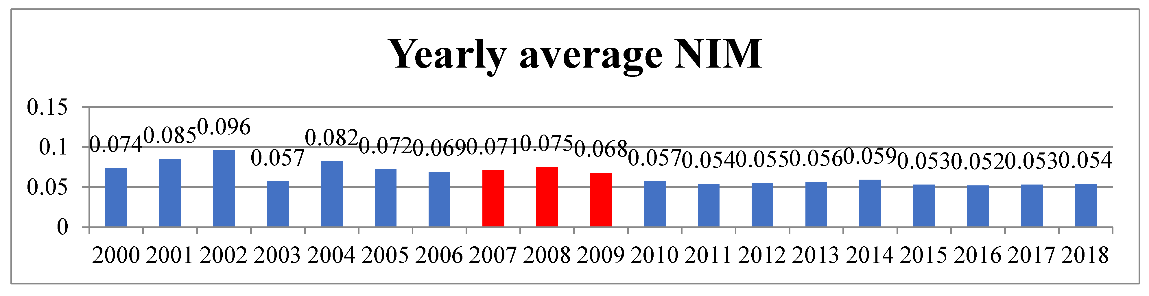
In this study, we assess the impact of the recent global financial crisis on bank margins and find the banking sector in EEs was significantly positively affected during the crisis. The yearly average net interest margin figure is presented below.

Figure 1 shows that the net interest margins were comparatively higher than the previous year during the crisis (2007 to 2009), and the aftermath. The average between 2000 and 2006 was around 7.6%, during the crisis it was 7.1%, but this rate reduced to 5.5% for the rest of the period (three red boldfaced bars represent a period of crisis).

3. Data, Variables, and Model

The data used in this study is collected from various sources: the data for the bank and industry-level determinants was downloaded from Bureau Van Dijk’s BankFocus database and made user-specific thereafter. The data for country-level determinants is composed of that from Aizenman et al. (2010) and Freedom_House (2017). Data for banking regulatory determinants was taken from Barth et al. (2013). Institutional variables are from the World Governance Indicators database of Kaufmann et al. (2011). Finally, among the macroeconomic indicators, Inflation and GDP were collected from the World Development Indicators (WDI) of the World Bank and monthly averages of daily money market interest rates taken from International Financial Statistics (IMF) and made user-specific thereafter. Below

Table 1. Determinants of the cost of financial intermediation: Variable definitions.

Variables	Symbol	Definition	Variable Reference	Data Source
Dependent Variables
Net Interest Margin	NIM1	Difference between interest income and interest expense over total earning assets	(Rahman et al. 2018)	BankFocus database
	NIM2	Difference between interest income and interest expense over total assets	(Rahman et al. 2018)	BankFocus
Independent Control Variables
Bank-Level
Govt. securities	GOVS	Investment in govt. securities to total assets	Author’s Idea	BankFocus
Cost Inefficiency	CINEY	Use stochastic frontier 4.1	(Rahman et al. 2021)	BankFocus
Operating Cost Ratio	OPCR	Operating expenses over total assets ratio	(Rahman et al. 2021)	BankFocus
Credit Risk	NPLTL	Non-performing loan to total loan ratio	(Rahman et al. 2021)	BankFocus
Credit Risk*SDint	NLMIR	NPL times SD of market interest rates	Author’s Calculation	BankFocus and Inter. Financial Stat. (IMF)
Capital Ratio	OETTA	Equity to total assets ratio	(Zheng et al. 2017)	BankFocus
Net Non-Interest Income Ratio	NNIR	Non-interest expense less non-interest revenue over total earning assets	(Rahman et al. 2017)	BankFocus
Opportunity Cost of Bank Reserves	OCR	Measured by the ratio of cash due from banks divided by total assets	Author’s Calculation	BankFocus
Size of Operations	LL	Logarithm of total loans	(Rahman et al. 2021)	BankFocus
Funding Strength	TLTD	Total loan to total deposit ratio	(Rahman et al. 2018)	BankFocus
Management Efficiency	CIR	Measured by the ratio of cost to income	(Rahman et al. 2017)	BankFocus
Industry-Level
Hirschman-Herfindahl Index	HHI	Sum of square of market share is a proxy for market concentration variable	(Rahman et al. 2021)	BankFocus and Authors’ calculations
Country-Level
Trilemma Index	TRMET	Composite of country scores in the area of Exchange Rate Stability, Monetary Independence, and Financial Openness4. For every measure, index ranges from 0 to 1 where a higher value indicates more Exchange Rate Stability, Monetary Independence, and Financial Openness	Author’s Idea	(Aizenman et al. 2010)
Market Openness	MKTOPN	Composite of country scores in the area of Trade Freedom, Investment Freedom, and Financial Freedom5. For every measure, index ranges from 0 to 1 where a higher value indicates more Trade Freedom, Investment Freedom, and Financial Freedom	Author’s Idea	Freedom_House (2017)
Regulatory-Level
Capital Stringency	CAPR	CAPR is an index of required capital that accounts for both initial and overall capital stringency. The index ranges from 0 to 10 where a higher value indicates more stringent capital requirements for banks in a country	(Barth et al. 2013)	Bank Regulation and Supervision Database, World Bank; (Barth et al. 2013)
Activity Restrictions	ACTR	This variable score reflects the level of regulatory restrictiveness for bank participation in securities, insurance, real estate activities, and owning other firms. Variable ranges from 4 to 16, with higher values, indicating greater restrictiveness	(Barth et al. 2013)	Bank Regulation and Supervision Database, World Bank; (Barth et al. 2013)
Supervisory Power	SPR	SPR is an index measuring the power of supervisory agencies specifying the extent to which these authorities could take actions against bank and board management, shareholders, and bank auditors. Variable ranges from 0 to 14, with higher values, indicating more supervisory power	(Barth et al. 2013)	Bank Regulation and Supervision Database, World Bank; (Barth et al. 2013)
Institutional-Level
Govt. Effectiveness	GVTETV	GVTETV is an index that reflects the perceptions of the quality of public services, the superiority of the civil service and the degree of its independence from political pressure, the quality of policy formulation and implementation, and the integrity of the government’s obligation to such policies. Variable ranges from −2.5 to 2.5, with higher values, indicating more Govt. Effectiveness	(Kaufmann et al. 2011)	(Kaufmann et al. 2011)
Rule of Law	ROL	ROL is an index that replicates the views of the extent to which peoples have confidence in and abide by the rules of society and in particular the quality of contract prosecution, property rights, the police, and the courts, as well as the possibility of crime and violence. Variable ranges from −2.5 to 2.5, with higher values, indicating more public-friendly law and enforcement	(Kaufmann et al. 2011)	(Kaufmann et al. 2011)
Macro-Level
SD of Market Interest Rates	SDMIR	Annualized standard deviation of monthly average of daily money market interest rates for an individual country	Author’s Calculation	Inter. Financial Statistics (IMF), and Authors’ calculations
Inflation, Consumer Prices (annual %)	INF	Annual rate of inflation (%)	(Rahman et al. 2020)	World Development Indicators (WDI)
GDP growth (annual %)	GDP	Annual growth of GDP	(Rahman et al. 2020)	World Development Indicators (WDI)

is a detailed explanation of the variables and data sources employed in our study.

3.1. Sample

The accounting data from a financial statement for commercial, investment, savings, cooperative, foreign, and bank holdings companies over the period 2000–2018 were collected from Bureau Van Dijk’s BankFocus database, and it encompasses only the active banks to avoid misleading information. All bank-level determinant values are measured in a million US dollars from the consolidated financial statement and are computed at fiscal year-end. Sample construction was started by erasing all bank observations with missing necessary financial data. The zero and negative figures for input and output measures of cost efficiency were also deleted since they required a log form of all data to run with SFA (Stochastic Frontier Analysis). Banks with less than three valid observations were deleted over the sample period. Finally, all bank-specific determinants were winsorized at one and ninety-nine percent to eliminate the outlier effects.

3.2. Measurement of Bank Net Interest Margin

Following the pioneering work of Ho and Saunders (1981), and its subsequent extension by several scholars, we appointed net interest margin (NIM1) as a dependent variable and defined it as the difference between interest income and interest expense divided by total earning assets. To test the sensitivity of our findings, we employed another proxy of net interest margin (NIM2) calculated as the difference between interest income and interest expense divided by total assets. Higher values of both of these measures represent the higher cost of financial intermediation and vice versa.

3.3. Bank-Level Control Variables

Following the previous literature, ten bank-level determinants, Govt. Securities (GOVS), Cost Inefficiency (CINEY), Credit Risk (NPLTL), Credit Risk*SDint (NLMIR), Capital Ratio (OETTA), Net Non-Interest Income Ratio (NNIR), Opportunity Cost of Bank Reserves (OCR), Size of Operations (LL), Funding Strength (TLTD) and Management Efficiency (CIR) are used to determine the bank interest margin. The detailed way of measuring the variables and data source is presented in Table 1, and for the references to the origin of variables, we suggested going through Table A1.

3.4. Industry-Level Variable

We used Hirschman-Herfindahl Index (HHI) in our model as a proxy for market power to capture its relationship with bank interest margin in EEs. It has been defined as the sum of squares of individual bank asset shares in the total banking sector assets for a country. Following, we expect a positive relationship with net interest margin (NIM) in EEs, explaining that the bank might enjoy monopoly power by demanding a higher spread when facing relatively inelastic demand and supply functions in the markets. The result is that it would hinder banking competitiveness. Since changes may occur in net interest margin during the global financial crisis 2007–2009, we employ a dummy variable, equal to 1 for the period of crisis and 0 otherwise, to estimate its impact on net interest margin by assessing a separately fixed effect regression.

3.5. Country-Level Determinants

Two variables are employed as proxies of country-level determinants. Trilemma Index is the composite of country scores in the area of Exchange Rate Stability (ERS), Monetary Independence (MI), and Financial Openness (FO) compiled by Aizenman et al. (2010). These indexes quantify the degree of achievement based on the three aspects of the ‘trilemma’ hypothesis (ERS) and are measured as the standard deviations of the monthly exchange rate between the home country and the base country. (MI) is communal of the annual correlation between the monthly interest rates of the home country and the base country6. (FO) index, also known as the Kaopen index measures the extent of openness in cross-border capital account transactions based on the existence of multiple exchange rates, restrictions on capital and current account transactions, and the requirement of the surrender of export proceeds. For every measure, the index ranges from 0 to 1 where a higher value indicates more Exchange Rate Stability, Monetary Independence, and Financial Openness, which leads us to predicted negative association with bank margins.

The market Openness index is the composite of country scores in the area of Trade Freedom (TF), Investment Freedom (IF), and Financial Freedom (FF) compiled by the Heritage Foundation. Where (TF) index quantifies the extent of control on imports and exports of goods and services, based on two inputs: the trade-weighted average tariff rate and nontariff barriers, (IF) index quantifies the extent of restrictions on foreign investment in a country based on seven broad areas. (FF) this index quantifies the extent of government control and interference in the financial sector based on five broad areas7. For every measure, the index ranges from 0 to 1 where a higher value indicates more market openness and is expected to be allied with lower margins.

3.6. Regulatory-Level Determinants

Three variables are employed as proxies of regulatory-level determinants. The data for Capital Stringency (CAPR), Activity Restrictions (ACTR), and Supervisory Power (SPR) determinants are collected from Barth et al. (2013). Since the data are compiled from the World Bank surveys on bank regulations and supervisions conducted in 1999, 2003, 2007, and 2011, we use data from the survey held in 1999 for bank observations over the year 2000 to 2002, in 2003 for bank observations over the year 2003 to 2006, in 2007 for bank observations over the year 2007 to 2010, and in 2011 for bank observations over the period 2011 to 2018. Capital Stringency is a sum of 10 questions8, which includes two sun-indices: initial and overall capital stringency index. CAPR index indicates the extent of capital requirements based on the quantity and quality9 of capital, sensitivity to credit, and market and operational risks. Moreover, it also reflects whether the regulatory authorities verified the sources of injecting capital and what types of losses are deducted to calculate the capital adequacy ratio. CAPR Index ranges from 0 to 10 where a higher value shows more stringent capital requirements and vice versa. By influencing the findings of Zheng et al. (2017), we also expect a negative association between CAPR and bank interest margin since well-capitalized banks suffered from lower bankruptcy costs and, hence the investments seem to be secure. As a result, the shareholders might expect a lower rate of return on equity; this may assist in reducing the bank margin.

ACTR index reflects the extent to which the banks face restrictions on non-traditional activities such as securities markets, insurance, real estate, and owning shares in nonbanking firms. Variable ranges from 4 to 16, with higher values indicating greater restrictiveness and vice versa. Following Poghosyan (2013), we expect a positive relationship between activity restrictions and bank margins, arguing that restrictions on market-based banking may hinder the banking system efficiency, which might induce the bank margins.

SPR is an index to measure the power of supervisory agencies specifying the extent to which these authorities could take action against bank and board management, shareholders, and bank auditors. Variables range from 0 to 14, with higher values indicating more supervisory power and vice versa. Since the stringent supervisory power ensures market discipline and a levelplaying field for the banking firm, it would assist in reducing the bank interest margins.

3.7. Institutional-Level Determinants

Two variables are employed as proxies of institutional-level determinants:

The data for institutional determinants such as Government Effectiveness (GVTETV) and Rule of Law (ROL) is collected from Worldwide Governance Indicators: World Bank, compiled by Kaufmann et al. (2011).

GVTETV is an index that reflects the perceptions of the quality of public services, the superiority of the civil service and the degree of its independence from political pressure, the quality of policy formulation and implementation, and the integrity of the government’s obligation to such policies. Variable ranges from −2.5 to 2.5; a higher index indicates better government effectiveness and is expected to be related to lower bank interest margins.

ROL is an index that replicates the views of the extent to which peoples have confidence in and abide by the rules of society and, in particular, the quality of contract prosecution, property rights, the police, and the courts as the possibility of crime and violence. Variable ranges from −2.5 to 2.5; a higher index indicates better rules of law and is expected to be related to lower bank interest margins

3.8. Macroeconomic-Level Determinants

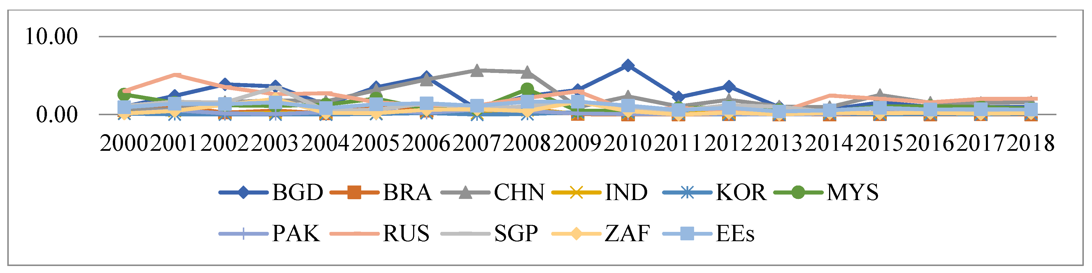
Following Ho and Saunders (1981), and its subsequent extension by Islam and Nishiyama (2016), we employed three determinants as a proxy of macroeconomic determinants such as standard deviation of money market interest rates (SDMIR), inflation, consumer prices (INF), and GDP growth (GDP). The SDMIR, INF, and GDP data have been collected from International Financial Statistics (IFS): IMF and World Development Indicators (WDI): World Bank, respectively. We calculate SDMIR as the annualized standard deviation of the monthly average of daily money market interest rates for an individual country to capture the impact of interest rate risk on bank interest margins. The banks might face the variation of money market rates with the inventory nature of the deposit fund and are expected to be positively related to bank interest margins. Figure 2 shows the standard deviation of money market interest rates for individual countries that we have selected in this study.

As shown in Table A1, several interested groups tested the impact of inflation and GDP growth on bank net interest margin. Among them, Tarus et al. (2012) argued that in the short-term, interest rates may not vary with inflationary adjustment, but in the medium and long-term, banks certainly adjust their interest rates to compensate for the inflationary premium and are expected to be positively related to bank interest margins. Likewise, the economic growth of an economy facilitate diverse investment opportunities for the banking sector, and therefore Islam and Nishiyama (2016) argued that the boost in economic growth generates various scope of investments and creates green fields for investors and bankers as well. This might help to do business in an accessible environment and thus may assist in charging lower bank margins.

3.9. Specified Model

Considering the limitations of Ho and Saunders’ (1981) dealership model, we develop the single-stage modified dealership model followed by Maudos and De Guevara (2004), who argued that the period considered in this study covers the years 2000 to 2018. The availability of annual observations for 19 years makes it impossible to apply the two-stage methodology, so we use the single-stage methodology.

The empirical specification of the augmented dealership model to be estimated for the determinants of net interest margins of banks in EEs takes the following linear form:

$${\mathrm{an}\mathrm{NIM}}_{\mathrm{ij},\mathrm{t}}=\mathrm{C}+{\displaystyle \sum }_{\mathrm{b}=1}^{\mathrm{B}}{\mathsf{\beta }}_{\mathrm{b}}{\mathrm{Y}}_{\mathrm{it}}^{\mathrm{b}}+{\mathsf{\beta }}_1\mathrm{Market}\mathrm{Power}\mathrm{j},\mathrm{t}+{\displaystyle \sum }_{\mathrm{c}=1}^{\mathrm{C}}{\mathsf{\beta }}_{\mathrm{c}}{\mathrm{Y}}_{\mathrm{it}}^{\mathrm{c}}+{\displaystyle \sum }_{\mathrm{r}=1}^{\mathrm{R}}{\mathsf{\beta }}_{\mathrm{r}}{\mathrm{Y}}_{\mathrm{it}}^{\mathrm{r}}+{\displaystyle \sum }_{\mathrm{i}=1}^{\mathrm{I}}{\mathsf{\beta }}_{\mathrm{i}}{\mathrm{Y}}_{\mathrm{it}}^{\mathrm{i}}+{\displaystyle \sum }_{\mathrm{m}=1}^{\mathrm{M}}{\mathsf{\beta }}_{\mathrm{m}}{\mathrm{Y}}_{\mathrm{it}}^{\mathrm{m}}+T{D}_{\mathrm{t}}+{\in }_{\mathrm{ijt}}$$

(6)

where i, j, and t subscripts stand for the bank, country, and year, respectively, and NIM is the net interest margin. C is a constant term. ${\mathrm{Y}}_{\mathrm{it}}$ with superscripts b, c, r, i, and m are the vectors of the bank, country, regulatory, institutional, and macroeconomic-specific determinants, respectively, and ${\in }_{\mathrm{ijt}}$ is an i.i.d. random error. The Hirschman-Herfindahl Index is used as the proxy of market power. Detailed definitions of all employed variables are given in Table 1. Bank-specific heterogeneity is seized by the fixed effects intercept term C and the time-specific variation is seized by a vector of time dummies TD. Moreover, we precede the following two tests for the econometric model:

First, we checked whether the effects of the individual determinants are fixed or random with the relevant Hausman test. The null hypothesis is that the individual effects of the control variables are random, and we reject the null hypothesis10 for equation 6, approving the evidence in favor of a fixed effect modeling. Second, we examined whether the bank-level heterogeneity exists in the model with the relevant White test. The null hypothesis is that the individual effects are homogeneous in nature and we reject the null hypothesis11 for equation 6, justified the estimate regression with robust standard error and clustered at the individual bank level. Next, as explained earlier, we address Lerner’s (1981) criticism of the dealership model with structural (Stochastic Frontier Analysis) calculation of production function (Cost Inefficiency) by employing the following model:

$${\mathrm{lnTC}}_{\mathrm{it}}=\mathrm{C}+{\displaystyle \sum }_{\mathrm{n}=1}^3{\mathsf{\beta }}_{\mathrm{n}}{\ln \mathrm{P}}_{\mathrm{nit}}+{\displaystyle \sum }_{\mathrm{k}=1}^3{\mathsf{\delta }}_{\mathrm{k}}{\mathrm{lnY}}_{\mathrm{kit}}+{\displaystyle \sum }_{\mathrm{n}=1}^3{\displaystyle \sum }_{\mathrm{m}=1}^3{\mathsf{\beta }}_{\mathrm{nm}}{\mathrm{lnP}}_{\mathrm{nit}}{\mathrm{lnP}}_{\mathrm{mit}}+{\displaystyle \sum }_{\mathrm{k}=1}^3{\displaystyle \sum }_{\mathrm{j}=1}^3{\mathsf{\delta }}_{\mathrm{kj}}{\mathrm{lnY}}_{\mathrm{kit}}{\mathrm{lnY}}_{\mathrm{jit}}+{\displaystyle \sum }_{\mathrm{n}=1}^3{\displaystyle \sum }_{\mathrm{k}=1}^3{\mathsf{\gamma }}_{\mathrm{nk}}{\mathrm{lnP}}_{\mathrm{nit}}{\mathrm{lnY}}_{\mathrm{kit}}+{\in }_{\mathrm{it}}$$

(7)

Here, the dependent variable is total cost (TC), which is defined as the sum of total interest, personal, and other operating expenses. In the specification of the inputs and outputs, we follow the intermediation approach and specify input prices (p) as the price of fund (PF), the price of labor (PL), and the price of capital (PC)12. The outputs (Y) are defined as total loans (TN), other earning assets (OEA), and total assets (TA), (Pessarossi and Weill 2015).

4. Empirical Analysis

4.1. Summary Statistics and Correlation Matrix

Table 2. Summary statistics and correlation matrix (Total sample).

6VARIABLES		1	2	3	4	5	6	7	8	9	10	11	12	13	14	15	16	17	18	19	20	21	22
NIM1	(1)	1
GOVS	(2)	0.03	1
CINEY	(3)	0.07	0.02	1
NPLTL	(4)	0.17	0.01	0.15	1
NLMIR	(5)	0.14	0.00	0.08	0.69	1
OETTA	(6)	0.34	0.01	−0.19	0.13	0.10	1
NNIR	(7)	0.71	0.02	0.02	0.11	0.11	0.16	1
OCR	(8)	−0.05	−0.01	−0.07	−0.03	−0.04	−0.09	−0.10	1
LL	(9)	−0.28	0.01	0.033	−0.06	−0.09	−0.52	−0.22	0.06	1
TLTD	(10)	0.00	0.00	−0.02	0.00	0.01	0.01	0.01	−0.02	0.00	1
CIR	(11)	0.09	−0.01	−0.28	0.09	0.08	0.19	0.36	−0.09	−0.48	0.02	1
HHI	(12)	−0.05	0.00	0.03	0.01	−0.01	−0.07	−0.04	0.02	0.19	0.00	−0.08	1
TRMET	(13)	0.01	−0.02	−0.32	−0.07	−0.14	0.13	0.03	0.04	−0.21	0.00	0.17	0.04	1
MKTOPN	(14)	0.05	−0.01	0.02	0.05	0.13	0.02	0.04	0.01	−0.07	−0.01	0.02	0.04	−0.11	1
CAPR	(15)	−0.02	−0.02	−0.08	−0.01	0.04	0.05	−0.01	0.00	−0.10	0.01	0.09	−0.05	−0.12	0.05	1
ACTR	(16)	−0.23	0.01	0.13	−0.03	−0.02	−0.27	−0.18	0.13	0.51	−0.01	−0.44	0.11	−0.21	−0.01	−0.11	1
SPR	(17)	0.03	0.03	0.54	0.10	0.01	−0.17	−0.03	−0.06	0.36	−0.02	−0.41	0.10	−0.28	0.01	−0.15	0.49	1
GVTETV	(18)	−0.16	0.01	0.20	0.02	−0.06	−0.16	−0.12	0.15	0.45	−0.01	−0.26	0.14	−0.06	−0.01	−0.01	0.34	0.31	1
ROL	(19)	−0.17	0.01	0.33	0.07	−0.03	−0.22	−0.13	0.07	0.54	−0.01	−0.32	0.13	−0.26	−0.05	0.04	0.41	0.46	0.89	1
SDMIR	(20)	0.04	0.00	−0.04	0.00	0.40	0.04	0.03	−0.04	−0.11	0.01	0.04	−0.01	−0.18	0.22	0.11	−0.01	−0.05	−0.14	−0.10	1
INF	(21)	0.15	−0.01	−0.20	−0.01	0.20	0.20	0.12	−0.07	−0.45	0.02	0.28	−0.05	−0.02	0.43	0.24	−0.40	−0.29	−0.47	−0.54	0.37	1
GDP	(22)	−0.12	0.00	0.05	−0.15	−0.26	−0.17	−0.16	0.06	0.23	−0.03	−0.36	0.05	0.05	−0.04	−0.14	0.46	0.32	0.09	0.11	−0.17	−0.34	1
MEAN		0.062	0.025	0.250	0.049	0.001	0.173	0.032	0.067	5.48	0.793	0.719	0.002	1.33	1.39	6.60	8.51	9.12	−0.17	−0.55	0.014	8.10	3.68
S.D.		0.057	0.038	0.238	0.081	0.001	0.133	0.059	0.072	2.75	2.95	0.29	0.02	0.20	0.225	1.30	1.91	2.18	0.447	0.478	0.016	3.77	4.39
MIN14		−2.2	0.002	0.013	0.000	0.00	−1.1	−2.2	0.00	−3.67	0.00	0.05	0.00	0.61	0.796	3.00	6.00	6.00	−0.81	−1.1	0.00	−0.77	−7.82
MAX		0.859	0.25	1.77	1.25	0.022	0.992	0.903	0.821	14.42	25.91	8.40	0.735	2.32	2.55	9.00	15.00	14.00	2.43	1.89	0.207	21.46	15.24
OBS		12,347		12,347		12,347		12,347		12,347		12,347		12,347		12,347		12,347		12,347		12,347

Note: Govt. Securities (GOVS), Cost Inefficiency (CINEY), Credit Risk (NPLTL), Credit Risk*SDint (NLMIR), Capital Ratio (OETTA), Net Non-Interest Income Ratio (NNIR), Opportunity Cost of Bank Reserves (OCR), Size of Operations (LL), Funding Strength (TLTD), Management Efficiency (CIR), Hirschman-Herfindahl Index (HHI), Trilemma Index (TRMET), Market Openness (MKTOPN), Capital Stringency (CAPR), Activity Restrictions (ACTR), Supervisory Power (SPR), Govt. Effectiveness (GVTETV), Rule of Law (ROL), SD of Market Interest Rates (SDMIR), Inflation (INF), and GDP growth (GDP).

and

Table 3. Mean of variables (Country-wise).

Variables	BGD	BRA	CHN	IND	KOR	MYS	PAK	RUS	SGP	ZAF
NIM1	0.0402	0.1033	0.0273	0.0322	0.0248	0.0254	0.0446	0.0672	0.0202	0.0645
GOVS	0.0230	0.0439	0.0278	0.01941	0.00553	0.01018	0.01284	0.02097	0.02824	0.03275
CINEY	0.1999	0.6808	0.2633	0.3394	0.2009	0.3187	0.3893	0.1565	0.2488	0.5083
NPLTL	0.0769	0.0881	0.0172	0.0454	0.0307	0.0571	0.1155	0.0429	0.0718	0.0628
NLMIR	0.0014	0.0010	0.00002	0.0011	0.0001	0.00003	0.0010	0.0007	0.0002	0.0003
OETTA	0.0765	0.1630	0.0861	0.0882	0.0813	0.1255	0.1502	0.2019	0.1665	0.1449
NNIR	0.0064	0.0593	0.0074	0.0072	0.0113	0.0054	0.0246	0.0367	0.0040	0.0050
OCR	0.0729	0.0153	0.1178	0.0511	0.0596	0.1417	0.0562	0.0657	0.0764	0.1364
LL	7.0496	6.4416	9.4795	7.9706	10.214	7.8112	6.2058	4.1805	8.5360	8.0142
TLTD	0.8548	0.82640	0.9440	0.56959	0.72130	0.90020	0.92021	0.71555	0.87902	0.77060
CIR	0.4906	0.6272	0.4092	0.4889	0.5945	0.5347	0.6890	0.8206	0.5315	0.5930
HHI	0.0040	0.0020	0.0033	0.0019	0.0038	0.0139	0.0156	0.0006	0.0265	0.0068
TRMET	1.3422	1.2008	1.4151	0.9588	1.4656	1.0989	1.0467	1.4013	2.0352	0.9945
MKTOPN	1.2689	1.3824	1.3199	1.4462	1.3374	1.3885	1.3857	1.3930	1.3271	1.3232
CAPR	5.7818	5.7101	4.4910	7.7877	7.1867	7.4171	7.9681	6.6903	6.9375	8.1073
ACTR	13.000	7.8309	12.789	11.0839	10.700	10.117	11.282	7.5270	9.8750	8.1631
SPR	11.109	13.424	10.721	10.2464	8.5933	11.126	13.106	7.8717	13.000	7.9227
GVTETV	−0.774	−0.078	0.1695	−0.0611	1.1452	1.0287	−0.717	−0.359	2.2025	0.4259
ROL	−0.775	−0.233	−0.389	0.0111	0.9690	0.5348	−0.839	−0.814	1.6961	0.1058
SDMIR	0.0223	0.0112	0.0012	0.0312	0.0020	0.0007	0.0086	0.0149	0.0021	0.0040
INF	7.2425	6.5368	2.6904	7.5814	1.9966	2.3688	7.6065	9.6417	2.2767	5.8616
GDP	6.1990	2.8491	8.5797	7.1576	3.4610	5.2102	4.2245	2.7272	5.7258	0.0645
OBS	197	1235	858	910	179	418	224	7914	134	278

deliver the descriptive statistics of net interest margin and its determinants for EEs and sample countries. The average net interest margin is 6.2%, with the highest in Brazil being 10% and the lowest in Singapore being 2%. The average investment in government securities as a portion of total assets is 2.5%, where the highest in Brazil is 4.3%, and the lowest in the Korean Republic is 0.05%. The overall mean cost inefficiency is 25%, which means substantial efficiency in the banks, averaging 75% of the total cost, suggesting that there is an opportunity to reduce the net interest margin by increasing the efficiency up to 25% of the total cost. Among the sample countries, Russian banking efficiency is the highest at 84.4%, while Brazil suffers from the lowest efficiency at 32%. The mean of the non-performing loan over the total loan is 4.9%, whereas the maximum in Pakistan is 11.5%, and the lowest in China is 1.7%. The average of equity over total assets is 17.3%, where the highest in Russia is 20%, and the lowest in Bangladesh is 7.6%. The banking sector of Bangladesh holds some nationalized banks whose owner’s equity to total assets is negative (Zheng et al. 2017), which would be a severe case that could turn into insolvency and require assistance from the lender as a last resort. The average market power is 0.02%, where the highest in Singapore is 2.6%, and the lowest is in India and Russia. The overall mean and sample countries’ mean indicates the banking sector in EEs is competitive, and the findings of this study proved it since HHI is insignificant as a determinant of NIM. As shown from the mean and standard deviation values, all bank, industry, country, regulatory, institutional, and macroeconomic-level determinants have a considerable variation across means. By countries, Bangladesh represents 2.6% of banks in our total sample, while Brazil, China, India, Korea Republic, Malaysia, Pakistan, Russian Federation, Singapore, and South Africa represent 9.6%, 10.56%, 6.2%, 2.4%, 5.5%, 3%, 56.70%, 1.4%, and 2%, respectively.

Further, Table 2 integrates the correlation matrix of dependent and explained control variables in EEs’ banks. The parallel correlation among the variables is reasonably small, advising that the explanatory power of selected variables as determinants of NIM can be distinguished at the time of total variation and thereafter. The highest correlation between NPLTL and NLMIR is 0.69, which indicates that the problem of multicollinearity is not undermining our results13.

4.2. Determinants of the Cost of Financial Intermediation: Main Specification

To analyze the determinants of the cost of financial intermediation, Equation (6) is estimated with fixed effect regression to address all proxies of bank, industry, country, regulatory, institutional, and macroeconomic determinants, which have been presented in

Table 4. Determinants of the cost of financial intermediation.

Variables	(1)	(2)	(3)	(4)	(5)	(6)	(7)	(8)
	NIM1
Bank-Level
GOVS	0.001 **	0.002 ***	0.001 ***	0.001 **	0.002 ***	0.001 ***	0.002 **	0.003 ***
CINEY	0.051 ***	0.053 ***	0.055 ***	0.051 ***	0.045 ***	0.051 ***	0.041 ***	0.043 ***
NPLTL	0.018 **	0.021 ***	0.018 **	0.018 **	0.020 ***	0.017 **	0.019 **	0.021 ***
NLMIR	−0.216	−0.369	−0.210	−0.216	−0.264	−0.188	−0.307	−0.263
OETTA	0.105 ***	0.106 ***	0.105 ***	0.105 ***	0.105 ***	0.105 ***	0.106 ***	0.105 ***
NNIR	0.584 ***	0.584 ***	0.584 ***	0.584 ***	0.584 ***	0.584 ***	0.584 ***	0.583 ***
OCR	0.047 ***	0.048 ***	0.047 ***	0.047 ***	0.048 ***	0.048 ***	0.047 ***	0.046 ***
LL	−0.001 *	−0.001	−0.001	−0.001 *	−0.001	−0.001 **	−0.001 **	−0.001
TLTD	−0.00001	−0.00001	−0.00001	−0.00002	−0.00002	−0.00001	−0.00002	−0.00001
CIR	−0.052 ***	−0.053 ***	−0.053 ***	−0.053 ***	−0.053 ***	−0.054 ***	−0.054 ***	−0.053 ***
Industry−Level
HHI	−0.016	−0.016	−0.016	−0.016	−0.016	−0.017	−0.014	-0.016
Country-Level
TRMET		−0.014 ***
MKTOPN			0.002 *
Regulatory-Level
CAPR				−0.001 *
ACTR					0.001 **
SPR						−0.001 **
Institutional-Level
GVTETV							−0.009 ***
ROL								−0.013 ***
Macro-Level
SDMIR	0.054 **	0.059 ***	0.052 **	0.054 **	0.051 **	0.055 **	0.038 *	0.061 ***
INF	0.00003	0.00002	0.00002	0.00002	0.0002	0.00003	0.00002	0.00002
GDP	−0.0001	−0.0002 **	−0.0001	−0.0001 *	−0.0001	−0.0001 *	−0.0001 *	−0.0001
Constant	0.050 ***	0.068 ***	0.047 ***	0.051 ***	0.042 ***	0.058 ***	0.056 ***	0.046 ***
Country dummies	Yes	Yes	Yes	Yes	Yes	Yes	Yes	Yes
Time dummies	Yes	Yes	Yes	Yes	Yes	Yes	Yes	Yes
R-squared	0.566	0.568	0.567	0.566	0.567	0.567	0.567	0.567
F-statistics (p-value)	439.70 (0.00)	487.68 (0.00)	484.11 (0.00)	483.65 (0.00)	484.53 (0.00)	484.46 (0.00)	485.57 (0.00)	485.66 (0.00)
Hausman Test, χ2 (p-value)	473.32 (0.00)	496.93 (0.00)	476.85 (0.00)	486.97 (0.00)	438.44 (0.00)	466.25 (0.00)	456.55 (0.00)	395.32 (0.00)
White Test, χ2 (p-value)	185.75 (0.00)	181.90 (0.00)	171.02 (0.00)	163.42 (0.00)	174.64 (0.00)	172.81 (0.00)	160.77 (0.00)	171.29 (0.00)
Observations	12,347	12,347	12,347	12,347	12,347	12,347	12,347	12,347
No of Banks	1335	1335	1335	1335	1335	1335	1335	1335

Note: Dependent Variable is NIM1 across all models. The table represents the regression output from the Fixed Effect estimation of the cost of financial intermediation determinants. ***, ** and * indicate significance at the 1%, 5% and 10% levels, respectively. Heteroskedasticity-robust standard errors clustered at the bank level are in parentheses. F-statistics (p-value) is the test for the goodness of fit of the model, while the Hausman test confirms the justification of using fixed effect estimation, and the White heteroskedasticity test justifies the use of robust standard error for the models. Variables definitions are presented in Table 1.

. Model 1 delivers the primary specification that estimates the impact of bank, industry, and macroeconomic determinants, and subsequently, models 2 to 8 are extended with alteration of country, regulatory and institutional determinants.

First, we consider the bank-specific determinants. Among them, our contributing variable GOVS plays a significant role in determining bank interest margins. As can be seen, there is a positive association between investment in govt. securities and the net interest margins across all models, arguing that even though the investment in govt. securities seem to be a risk-free investment, but there might be some opportunity costs, which could lead to charging a higher cost of intermediation. In concrete, a 1% increase in the investment in govt. securities would increase the net interest margin by around 0.02 basis points. As expected, we find that greater cost inefficiency (CINEY) in the production function might positively impact the bank’s net interest margins in EEs (Rahman et al. 2017). Supporting the efficient-structure hypothesis, we argued that the differences in interest margins are attributable to differences in operational efficiency among the banks and lead to an adverse association between operational efficiency and interest margins. Consequently, customers pay more to the less efficient banks in EEs. Non-performing loans as a portion of the total loan (NPLTL), which are captured as the credit risk of the banking firm, are found to be positive and statistically significant as a determinant of NIM through all models, suggesting that the higher non-performing loans increase the cost of the loan which may turn into the higher cost of capital in the form of bad debt (Rahman et al. 2021). Subsequently, the banks pass on this cost to the borrowers by charging higher interest rates on loans. The interaction of credit and interest rate risk (NLMIR) appeared negative but statistically insignificant in our study.

Equity to total assets (OETTA) significantly impacts bank margins, indicating that well-capitalized banks charge higher margins than lower-capitalized banks (Rahman et al. 2018). Based on the standard corporate finance theory of capital structure, we argued that equity is an expensive source of capital and a percentage increase in equity as capital increases the overall weighted average cost of capital (WACC) for the banks. Besides, the framework of Zheng et al. (2017) argued with another aspect of the capital structure theory that bank shareholders would not always expect a higher return from well-capitalized banks since with the increase in bank capital, the probability of expected default would reduce, and the banks are considered safer. However, the findings of this paper support our hypothesis that risk-averse banks charge higher net interest margins.

As expected, an increase in non-interest expenses as a portion of earning assets (NNIR) increases the bank interest margins. Thus the relationship is positive and highly significant across all models. Idle money in the form of reserve or cash over total assets ratio (OCR) and bank net interest margins are positively related, and the relationship is statistically significant at a 1% level. Since the increase in the cost of holding money will cause an increase in bank interest margins, subsequently, banks shift this cost burden to the clients (Rahman et al. 2017). The size of operation (LL) appeared to have a negative relationship with bank interest margin but was statistically insignificant in almost all models, arguing that the transaction economies or diseconomies of scale are not noteworthy in EEs’ banks. The total loan to total deposit (TLTD) ratio, which is captured as the finding strength of the banks, is negatively associated with bank interest margin through all models, but the relationship is ignorable. The cost-to-income ratio (CIR), which captures the management efficiency of the banks, enters negatively and significantly into EEs regressions, similar to (Rahman et al. 2017; Rahman et al. 2021; Rahman et al. 2018; Zheng et al. 2017). A higher ratio is associated with lower management efficiency. As expected, efficient management seems to be special, and the banks might charge more for their specialty.

Second, we consider the industry-specific determinants. As can be seen, Marker power (HHI) of banking in Emerging Economies (EEs) and net interest margins enters negatively associated but are found to be statistically insignificant. The findings disprove our initial prediction that higher market power will create an opportunity for charging higher bank interest margins. Instead, these divergent findings proved that, as evidenced by descriptive statistics; the banking industry of EEs’ has undergone a harsh competitive environment.

Third, Table 4 also analyzes the impact of country-level factors when controlling for bank, industry, and macroeconomic-specific determinants (models 2–3). As can be seen, the estimated results document a strong negative relationship between Trilemma Indices (TRMET) and bank interest margins. Thus, this proved our initial hypothesis and justified our research contribution. As explained earlier, Trilemma Index is the composite of country scores in the area of Exchange Rate Stability (ERS), Monetary Independence (MI), and Financial Openness (FO), and therefore, we argue that the more stable exchange rate, monetary systems, and financial openness create an opportunity for banks to reduce their interest rate risk through conducting their banking activities with a diversified and stable environment, which might help to reduce the bank interest margins.

To capture the scenario of market-based banking in EEs, we also consider Market Openness (MKTOPN) and found a positive association with bank interest margin. This finding disproved our initial hypothesis but justified its importance as a determinant of bank interest margins, which was not considered in the previous literature. As explained earlier, Market Openness is the composite of country scores in the area of Trade Freedom (TF), Investment Freedom (IF), and Financial Freedom (FF). One possible reason behind the divergent findings may be more freedom in trade, investment, and financial domains, the banks need to cover a wide range of activities, which might induce the personnel and administrative costs in operational procedures. Thus, the banks need to charge more to compensate for the higher operational costs. Among the regressions, the coefficient of Cost Inefficiency (model 3) is the largest (0.055), with market openness delivering documentation in favor of our argument.

Fourth, Table 4 also analyzes the impact of regulatory-level variables when controlling for bank, industry, and macroeconomic-specific determinants (models 4–6). As can be seen, Capital Stringency (CAPR) and Supervisory Power (SPR) enter negative and significant into the regressions, contrary to (Rahman et al. 2021). These results suggest that the regulatory restriction in capital and market discipline significantly affects bank interest margins. Economically speaking, a one standard deviation change in the Capital Stringency index (1.30) is associated with a change in net interest margin (NIM) of 0.0013 (0.001 × 1.30), where the mean NIM is 6.2%. These findings are consistent with the ‘public view’ hypothesis, whereby regulation is for the betterment of the public, not for a group of interested people. In contrast, it is opposite to the ‘private view’ hypothesis, whereby regulation is for the interested groups (i.e., the banks themselves to create managerial self-interest or the politically well-connected) rather than general people. Therefore, we deemed the banks operating with lower margins might significantly influence social well-being by making a reliable relationship with citizens.

Next, restrictions on non-traditional activities (ACTR), such as securities underwriting, insurance undertakings, real estate, and owning shares in nonbanking firms, have significant positive impacts on bank margins and are consistent with the findings of (Asli Demirgüç-Kunt et al. 2004; Poghosyan 2013). The existence of structural non-bank financial institutions in EEs deserves the participation of bank financial institutions to create a more synergic and competitive financial sector that might assist in reducing bank interest margins. Fifth, Table 4 also analyzes the impact of institutional-level factors when controlling for bank, industry, and macroeconomic-specific determinants (models 7–8). Consistent with the findings of Asli Demirgüç-Kunt et al. (2004) and Poghosyan (2013), the estimated results document a robust negative association between the institutional framework and bank interest margins. As reported, Govt. Effectiveness (GVTETV) and Rule of Law (ROL) enter negative and with a highly significant (at 1% level) coefficient in models 7 and 8, showing that the countries with a sound institutional quality have a significant positive role in the banking sector in reducing bank interest margins. Interestingly, among the regressions, the coefficient of investment in Govt. Securities (GOVS) enters highest with Govt. Effectiveness and Rule of Law. Besides, the coefficient of Cost Inefficiency comes lowest with Govt. Effectiveness and Rule of Law justify our argument that better institutional quality could promote the banking sector to operate in an efficient and competitive environment. Finally, we consider the macroeconomic-specific determinants. Among the variables, we found that the rate of Inflation (INF) and GDP growth (GDP) have no significant association in determining bank interest margins (Rahman et al. 2017; Rahman et al. 2018). However, these findings proved our initial hypothesis, that the severity of an impact on bank margins was immaterial. Alternatively, the standard deviation of money market interest rates (SDMIR) and net interest margins are positively and statistically significantly related. That is, if the interest rates risk increases by 1%, then we can expect five basis points (around) increase in the bank interest margins. Moreover, since the bank faces transaction uncertainty derived from the inventory nature of channeling money, they set their interest rates after compensating for the volatility of interest rates and thus enhance the bank interest margins.

4.3. Elasticity: Alternative Specification

We perform several robustness tests to confirm the main results further. Among them,

Table 5. Elasticity: Alternative variables (NIM2 and OPCR instead of NIM1 and CINEY).

Variables	(1)	(2)	(3)	(4)	(5)	(6)	(7)	(8)
	NIM2
Bank-level
GOVS	0.004 ***	0.003 ***	0.002 ***	0.002 ***	0.003 ***	0.002 ***	0.003 ***	0.004 ***
OPCR	0.016 ***	0.017 ***	0.018 ***	0.016 ***	0.016 ***	0.016 ***	0.017 ***	0.016 ***
NPLTL	0.003	0.005	0.002	0.003	0.005	0.002	0.004	0.007
NLMIR	−0.252	−0.360	−0.245	−0.252	−0.351	−0.242	−0.372	−0.376
OETTA	0.076 ***	0.076 ***	0.076 ***	0.075 ***	0.076 ***	0.076 ***	0.076 ***	0.075 ***
NNIR	0.426 ***	0.426 ***	0.426 ***	0.426 ***	0.426 ***	0.426 ***	0.426 ***	0.425 ***
OCR	0.021 ***	0.021 ***	0.021 ***	0.022 ***	0.019 ***	0.021 ***	0.021 ***	0.022 ***
LL	−0.001 ***	−0.001 ***	−0.001 ***	−0.001 ***	−0.001 *	−0.001 ***	−0.001 ***	−0.001**
TLTD	−0.00001	−0.00001	−0.00001	−0.00002	−0.00001	−0.00001	−0.00001	−0.00002
CIR	−0.045 ***	−0.045 ***	−0.045 ***	−0.045 ***	−0.045 ***	−0.045 ***	−0.045 ***	−0.044 ***
Industry-Level
HHI	−0.014	−0.014	−0.014	−0.013	−0.014	−0.014	−0.012	−0.015
Country-Level
TRMET		−0.010 ***
MKTOPN			0.002 **
Regulatory-level
CAPR				0.001 *
ACTR					0.002 ***
SPR						−0.001 **
Institutional-Level
GVTETV							−0.009 ***
ROL								−0.023 ***
Macro-Level
SDMIR	0.039 **	0.042 **	0.038 **	0.040 **	0.036 **	0.040 **	0.025	0.053 ***
INF	0.00004	0.00003	0.00004	0.00003	0.00004	0.00004	0.00003	0.0001 *
GDP	−0.0003 **	−0.0002 **	−0.0003 **	−0.0003 **	−0.0003 **	−0.0004 **	−0.0004 **	−0.0002 *
Constant	0.061 ***	0.074 ***	0.058 ***	0.060 ***	0.046 ***	0.064 ***	0.064 ***	0.049 ***
Country dummies	Yes	Yes	Yes	Yes	Yes	Yes	Yes	Yes
Time dummies	Yes	Yes	Yes	Yes	Yes	Yes	Yes	Yes
R-squared	0.538	0.539	0.538	0.538	0.539	0.538	0.539	0.542
F-statistics (p-value)	448.81 (0.00)	402.06 (0.00)	399.54 (0.00)	398.97 (0.00)	402.01 (0.00)	398.94 (0.00)	401.66 (0.00)	408.47 (0.00)
Observations	12,347	12,347	12,347	12,347	12,347	12,347	12,347	12,347
No of Banks	1335	1335	1335	1335	1335	1335	1335	1335

Note: Dependent Variable is NIM2 across all models. The table represents the regression output from the Fixed Effect estimation of the cost of financial intermediation determinants. ***, ** and * indicate significance at the 1%, 5% and 10% levels, respectively. Heteroskedasticity-robust standard errors clustered at the bank level are in parentheses. Variables definitions are presented in Table 1.

represents the robust findings of our main specified model of determinants of bank interest margins after considering Net Interest Margin (NIM2) and Operating Cost Ratio (OPCR) as alternative measures of Net Interest Margin (NIM1) and Cost Inefficiency (CINEY), respectively. Net Interest Margin (NIM2) has been calculated as the ratio of net interest income over total assets. In contrast, the Operating Cost Ratio (OPCR) has been calculated as the ratio of operating expenses to total assets. Maudos and De Guevara (2004) first respond the Lerner’s (1981) criticism of the dealership model15 by explicitly incorporating the non-structural calculation of Cost Inefficiency as simply the accounting ratio of operating expenses to total assets and proved the model empirically. Nevertheless, we addressed the Lerner (1981) criticism of the dealership model with the structural framework (SFA) of Cost Inefficiency; then, we checked the degree of robustness of such criticism with the non-structural framework (accounting ratio) of Cost Inefficiency, which may create a new dimension to the existing literature.

However, using (NIM2) and (OPCR) as alternative measures of net interest margin and cost inefficiency, we found neither changes in sign nor significant changes in coefficient values of the explanatory variables. Thus, the reported results in Table 4 confirm that the findings obtained for the main specified model, Equation (6), remain valid.

4.4. Impact of Global Financial Crisis (GFC)

Following Poghosyan (2013), we add the global financial crisis dummy variable with the main specified model, Equation (6), using fixed effect regression to examine whether the bank interest margins were affected during the crisis. The reported results in

Table 6. Impact of the global financial crisis.

Variables	(1)	(2)	(3)	(4)	(5)	(6)	(7)	(8)
	NIM1
Bank-level
GOVS	0.002 ***	0.002 ***	0.003 ***	0.003	0.002 ***	0.003 ***	0.002 ***	0.003 ***
CINEY	0.052 ***	0.055 ***	0.056 ***	0.053 ***	0.048 ***	0.052 ***	0.041 ***	0.045 ***
NPLTL	0.019 ***	0.024 ***	0.019 ***	0.020 ***	0.020 ***	0.018**	0.020 ***	0.021 ***
NLMIR	−0.254	−0.485	−0.249	−0.264	−0.273	−0.226	−0.369	−0.274
OETTA	0.105 ***	0.105 ***	0.105 ***	0.105 ***	0.105 ***	0.105 ***	0.105 ***	0.105 ***
NNIR	0.584 ***	0.583 ***	0.583 ***	0.584 ***	0.584 ***	0.584 ***	0.584 ***	0.583 ***
OCR	0.047 ***	0.049 ***	0.047 ***	0.048 ***	0.048 ***	0.048 ***	0.048 ***	0.046 ***
LL	−0.001 **	−0.001 *	−0.001 *	−0.001 **	−0.001	−0.001 ***	−0.001 ***	−0.001*
TLTD	−0.00002	−0.00001	−0.00001	−0.00002	−0.00001	−0.00002	−0.00002	−0.00002
CIR	−0.053 ***	−0.053 ***	−0.053 ***	−0.053 ***	−0.053 ***	−0.054 ***	−0.053 ***	−0.053 ***
Industry-Level
HHI	−0.016	−0.016	−0.016	−0.016	−0.016	−0.017	−0.013	−0.016
Crisis dummy	0.002 **	0.003 ***	0.002 ***	0.002 ***	0.002 **	0.002 ***	0.002 ***	0.002 ***
Country-Level
TRMET		−0.018 ***
MKTOPN			0.003 **
Regulatory- level
CAPR				−0.001 *
ACTR					0.002 ***
SPR						−0.001 **
Institutional-Level
GVTETV							−0.010 ***
ROL								−0.011 ***
Macro-Level
SDMIR	0.042 *	0.038 *	0.040 *	0.038 *	0.044 *	0.043 *	0.021	0.054 **
INF	0.00003	0.0002 **	0.00003	0.00004	0.00004	0.00003	0.00003	0.00003
GDP	−0.0001	−0.0002 **	−0.0001	−0.0001	−0.0002	−0.0001 **	−0.0001 *	−0.0001
Constant	0.051 ***	0.074 ***	0.047 ***	0.053 ***	0.045 ***	0.059 ***	0.057 ***	0.046 ***
Country dummies	Yes	Yes	Yes	Yes	Yes	Yes	Yes	Yes
Time dummies	No	No	No	No	No	No	No	No
R-squared	0.567	0.569	0.567	0.567	0.567	0.567	0.568	0.567
F-statistics (p-value)	784.64 (0.00)	741.28 (0.00)	736.07 (0.00)	735.81 (0.00)	735.77 (0.00)	736.37 (0.00)	737.87 (0.00)	736.66 (0.00)
Observations	12,347	12,347	12,347	12,347	12,347	12,347	12,347	12,347
No of Banks	1335	1335	1335	1335	1335	1335	1335	1335

Note: Dependent Variable is NIM1 across all models. The bold-faced crisis dummy is the specially observed variable regarding the impact of the recent global financial crisis from 2007 to 2009 as 1, 0 otherwise. The table represents the regression output from the Fixed Effect estimation of the cost of financial intermediation determinants. ***, ** and * indicate significance at the 1%, 5% and 10% levels, respectively. Heteroskedasticity-robust standard errors clustered at the bank level are in parentheses. Variables definitions are presented in Table 1.

suggest that the crisis positively affected the bank margin. Graphically, Figure 1 provides supporting evidence in favor of econometric findings that the bank margin was increased during the crisis in the EEs banking sector. However, Table 6 also confirms that the signs and coefficients of the explanatory variables remain qualitatively unchanged compared to Table 4 when accounting for the impact of the crisis. That is because we captured the year-fixed effect with the proxy of year dummies in the main specification.

4.5. Dropping the Contributing Variables and Endogeneity

The reported results in

Table 7. Dropping the contributing variables and Endogeneity.

Variables	Dropped (GOVS)	Dropped (GOVS)	Dropped (TRMET)	Dropped (MKTOPN)	CINEY (First Stage)	NIM1 (Second Stage)
					Endogeneity test: Instrumental variable regressions
	(1)	(2)	(3)	(4)	(5)	(6)
CINEY	0.053 ***	0.051 ***	0.052 ***	0.051 ***		0.051 ***
OPCR					0.006 ***
GOVS			0.002 ***	0.003 ***	−0.001 *	0.002 ***
TRMET	−0.014 ***
MKTOPN		0.002*
NPLTL	0.021 ***	0.018 **	0.018 **	0.018 **	−0.067 ***	0.018 **
NLMIR	−0.370	−0.210	−0.216	−0.216	3.285 ***	−0.216
OETTA	0.106 ***	0.106 ***	0.105 ***	0.105 ***	−0.001	0.105 ***
NNIR	0.584 ***	0.584 ***	0.584 ***	0.584 ***	0.005	0.584 ***
OCR	0.048 ***	0.047 ***	0.047 ***	0.047 ***	−0.019 ***	0.047 ***
LL	−0.001	−0.001	−0.001 *	−0.001 *	−0.005 ***	−0.001 *
TLTD	−0.00002	−0.00002	−0.00001	−0.00001	0.00004	−0.00001
CIR	−0.053 ***	−0.053 ***	−0.053 ***	−0.053 ***	−0.006 ***	−0.053 ***
HHI	−0.016	−0.016	−0.016	−0.016	0.066 ***	−0.016
SDMIR	0.059 ***	0.052 **	0.055 **	0.054 **	−0.122 ***	0.054 **
INF	0.00002	0.00003	0.00001	0.00003	0.00004	0.00003
GDP	−0.0002 **	−0.0001	−0.0001	−0.0001	−0.0002	−0.0002
Constant	0.068 ***	0.047 ***	0.051 ***	0.050 ***	0.284 ***	0.050 ***
Country dummies	Yes	Yes	Yes	Yes	Yes	Yes
Time dummies	Yes	Yes	Yes	Yes	Yes	Yes
R-squared	0.547	0.559	0.552	0.557	0.197	0.566
F-statistics (p-value)	493.88 (0.00)	510.02 (0.00)	498.92 (0.00)	469.70 (0.00)	470.85 (0.00)	483.70 (0.00)
Observations	12,347	12,347	12,347	12,347	12,347	12,347
No of Banks	1335	1335	1335	1335	1335	1335

Note: Dependent Variable is NIM1 for models 1–4 and 6; Cost inefficiency is the dependent variable in model 5. All models are estimated using Fixed Effect estimation. p-values are computed by the heteroskedastic-robust standard errors clustered at the bank level and are presented in parenthesis. ***, **, * represent statistical significance at 1%, 5%, and 10% levels, respectively. Detailed definitions of the variables are presented in Table 1.

(models 1–4) justify the contribution of this study to existing literature. As explained earlier, we contribute to the present literature in several ways; we have considered an investment in govt. securities to total assets (GOVS) as bank-level determinants, then Trilemma Index (TRMET) and Market openness (MKTOPN) as country-level determinants were not reported in the past literature. Therefore, the statistical significance of these variables as the determinants of bank interest margins has been proved. Moreover, we checked the intense impact on bank interest margin by dropping those variables one-by-one from the main specified model Equation (6). Citing the Islam and Nishiyama (2016) framework, we have confirmed the validation of the inclusion of these variables in our estimated Equation (6) by checking the R². In columns (1–2), where we exclude the GOVS variable, the R² is 0.547 and 0.559, while in columns (2–3) of Table 3, where we include the GOVS variable, the R² is 0.568 and 0.567. Thus the absences of the GOVS variable have a measurable impact on R², proving that the investment in govt. securities plays a significant role in determining bank interest margins. Moreover, reported results in columns (3–4) of Table 7 compared to columns (2–3) of Table 4 show that when we exclude the contributing variables (TRMET) and (MKTOPN) from baseline model Equation (6), the R² went down 0.568 to 0.552 as of 0.567 to 0.557. That also justifies the significant impact of the Trilemma Index and Market openness on bank interest margins in EEs.

Next, we turn to the endogeneity test. The theoretical relationship between net interest margin and cost inefficiency in the previous literature (Agapova and McNulty 2016) suggests that we need to address the possible concern with the results of endogeneity between them. To address this possibility, we follow the Ashraf (2017) instrumental variable approach for the main specification (Model 1 of Table 4), and the results are reported in Models 5 and 6 of Table 7. Finally, citing the arguments of Baum et al. (2003) that an instrument must satisfy the relevance and exogeneity conditions16, we use the Operating Cost Ratio (OPCR) as an instrument for Cost Inefficiency (CINEY). The more cost in the operational procedure increases the operational inefficiency on the one hand while addressing the ‘efficiency wage’ theory that higher operating costs, especially higher personnel pay, could hire skilled staff, and it would relate to greater productivity (Tan 2016). However, the first-hand logic is straightforward. The increased operational procedure cost involved the largest gap between asks and bid price, which might also induce inefficiency and bank interest margins. Consistent with the arguments, the OPCR variable enters positive and significant with CINEY in the first stage regression in Model 5. In Model 6, the CINEY comes positive and significant with Net Interest Margins (NIM1) in second-stage regression. These findings confirm that endogeneity is less important in the main specification.

4.6. Regression for BRICS Block and Dropped Russia from Whole Samples

BRICS (Brazil, Russia, India, China, and South Africa) are the top 10 emerging economies in the world. This block accounts for 20% of the world’s GDP and 42.59% of the world’s population, with more than a quarter of the world’s land (Samargandi and Kutan 2016). The rapid growth post-millennium up to 2015 averaged 7.96%, and the significant influences on the global economy have been intensifying day by day. Mainly, the early recovery of the BRICS economies17 after the financial tsunami of 2007–2008 and their relatively smooth banking sectors provide a reasonable experimental opportunity to study the determinants of bank interest margins. In this study, BRICS economies contain 85.06% of total observations, which raises a question; the results may be biased due to large observations from selected economies. Thus, we re-estimate Equation (6) using fixed effect regression and the results are reported in

Table 8. Regression for BRICS region.

Variables	(1)	(2)	(3)	(4)	(5)	(6)	(7)	(8)
	NIM1
Bank-Level
GOVS	0.001 **	0.001 **	0.002 **	0.002 **	0.002 **	0.001 **	0.002 **	0.001 **
CINEY	0.057 ***	0.061 ***	0.062 ***	0.058 ***	0.052 ***	0.059 ***	0.044 ***	0.050 ***
NPLTL	0.006	0.009	0.006	0.006	0.007	0.003	0.007	0.008
NLMIR	0.269	0.138	0.290	0.268	0.231	0.337	0.173	0.230
OETTA	0.104 ***	0.105 ***	0.104 ***	0.104 ***	0.104 ***	0.104 ***	0.104 ***	0.104 ***
NNIR	0.596 ***	0.596 ***	0.595 ***	0.596 ***	0.595 ***	0.596 ***	0.596 ***	0.595 ***
OCR	0.048 ***	0.049 ***	0.048 ***	0.048 ***	0.049 ***	0.050 ***	0.049 ***	0.048 ***
LL	−0.001 *	−0.001	−0.001	−0.001	−0.001	−0.001 **	−0.001 **	−0.001
TLTD	−0.00001	−0.00001	−0.00002	−0.00002	−0.00001	−0.00001	−0.00001	−0.00001
CIR	−0.062 ***	−0.062 ***	−0.062 ***	−0.062 ***	−0.062 ***	−0.064 ***	−0.063 ***	−0.062 ***
Industry-Level
HHI	0.038	0.043	0.038	0.038	0.038	0.033	0.044	0.036
Country-Level
TRMET		−0.019 ***
MKTOPN			0.003 **
Regulatory-Level
CAPR				−0.002 *
ACTR					0.001 **
SPR						−0.001 ***
Institutional-Level
GVTETV							−0.010 ***
ROL								−0.010 ***
Macro-Level
SDMIR	0.036	0.043 *	0.034	0.035	0.033	0.037	0.017	0.042 *
INF	0.00004	0.0001 *	0.0001	0.0001	0.00004	0.0001	−0.00004	−0.00004
GDP	−0.0001	0.0001	−0.0002	−0.0002	−0.0001	0.0003	0.0003	−0.0001
Constant	0.058 ***	0.082 ***	0.054 ***	0.059 ***	0.053 ***	0.072 ***	0.065 ***	0.054 ***
Country dummies	No	No	No	No	No	No	No	No
Time dummies	Yes	Yes	Yes	Yes	Yes	Yes	Yes	Yes
R-squared	0.576	0.577	0.576	0.584	0.575	0.572	0.579	0.571
F-statistics (p-value)	497.45 (0.00)	449.85 (0.00)	444.88 (0.00)	444.25 (0.00)	444.56 (0.00)	446.38 (0.00)	446.40 (0.00)	445.28 (0.00)
Observations	9382	9382	9382	9382	9382	9382	9382	9382
No of Banks	1136	1136	1136	1136	1136	1136	1136	1136

Note: Dependent Variable is NIM1 across all models. The table represents the regression output from the Fixed Effect estimation of the cost of financial intermediation determinants. p-values are computed by the heteroskedastic-robust standard errors clustered at the bank level and are presented in parenthesis. ***, **, * represent statistical significance at 1%, 5%, and 10% levels respectively. Detailed definitions of the variables are presented in Table 1.

, showing that the findings are qualitatively unchanged when we run the separate regression for the BRICS region, confirming our main results are unbiased due to the large sample from the selected countries.

Moreover, we re-estimated Equation (6) using fixed effect regression after dropping Russia (56.70% of total observation) from the whole sample, and the results are reported in

Table 9. Dropping Russia from the whole sample.

Variables	(1)	(2)	(3)	(4)	(5)	(6)	(7)	(8)
	NIM1
Bank-Level
GOVS	0.008 *	0.007 *	0.008 **	0.008 *	0.007 **	0.006 *	0.005 **	0.006 *
CINEY	0.040 ***	0.039 ***	0.041 ***	0.037 ***	0.037 ***	0.040 ***	0.041 ***	0.035 ***
NPLTL	0.042 ***	0.041 ***	0.043 ***	0.041 ***	0.043 ***	0.042 ***	0.042 ***	0.042 ***
NLMIR	0.543	0.562	0.469	0.551	0.493	0.542	0.555	0.526
OETTA	0.117 ***	0.117 ***	0.117 ***	0.116 ***	0.117 ***	0.117 ***	0.117 ***	0.116 ***
NNIR	0.987 ***	0.987 ***	0.987 ***	0.987 ***	0.987 ***	0.987 ***	0.987 ***	0.986 ***
OCR	0.023 **	0.023 **	0.023 **	0.022 **	0.025 ***	0.023 **	0.023 **	0.023 **
LL	−0.003 ***	−0.003 ***	−0.002 ***	−0.003 ***	−0.003 ***	−0.003 ***	−0.003 ***	−0.003 ***
TLTD	−0.00002	−0.00003	−0.00004	−0.00004	−0.00003	−0.00003	−0.00002	−0.00002
CIR	−0.053 ***	−0.053 ***	−0.053 ***	−0.053 ***	−0.053 ***	−0.053 ***	−0.053 ***	−0.053 ***
Industry-Level
HHI	−0.038 **	−0.038 **	−0.039 **	−0.038 **	−0.039 **	−0.038 **	−0.038 **	−0.038 **
Country-Level
TRMET		−0.001 **
MKTOPN			0.004 **
Regulatory-Level
CAPR				−0.001 *
ACTR					0.001 **
SPR						−0.003 **
Institutional-Level
GVTETV							−0.002 *
ROL								−0.006 *
Macro-Level
SDMIR	−0.006	−0.007	−0.007	−0.003	−0.006	−0.006	−0.004	−0.003
INF	0.00002	0.00002	0.00001	0.00001	0.00001	0.00001	−0.00001	−0.00001
GDP	−0.0001	−0.0002	−0.0002	−0.0001	−0.0002	−0.0001	−0.0001	−0.0001
Constant	0.046 ***	0.045 ***	0.036 ***	0.045 ***	0.039 ***	0.046 ***	0.045 ***	0.047 ***
Country dummies	No	No	No	No	No	No	No	No
Time dummies	Yes	Yes	Yes	Yes	Yes	Yes	Yes	Yes
R-squared	0.874	0.875	0.848	0.847	0.849	0.842	0.857	0.846
F-statistics (p-value)	937.25 (0.00)	954.46 (0.00)	956.70 (0.00)	955.88 (0.00)	955.38 (0.00)	949.40 (0.00)	954.49 (0.00)	955.63 (0.00)
Observations	3715	3715	3715	3715	3715	3715	3715	3715
No of Banks	578	578	578	578	578	578	578	578

Note: Dependent Variable is NIM1 across all models. The table represents the regression output from the Fixed Effect estimation of the cost of financial intermediation determinants. p-values are computed by the heteroskedastic-robust standard errors clustered at the bank level and are presented in parenthesis. ***, **, * represent statistical significance at 1%, 5%, and 10% levels respectively. Detailed definitions of the variables are presented in Table 1.

. However, estimating the separate regression after dropping Russia, we found no changes in signs and no significant changes in coefficient values of determinants, confirming our main results are unbiased due to the large sample from Russia.

4.7. Sensitivity Analysis: Methodological Issues

To confirm the main results (Table 4) derived from Equation (6) are unbiased due to the methodological issue, a number of additional estimation techniques, pooled panel OLS, random effect, and dynamic panel system GMM18 estimation have been performed, and the results are reported in

Table 10. Pooled panel OLS regression.

Variables	(1)	(2)	(3)	(4)	(5)	(6)	(7)	(8)
	NIM1
Bank-Level
GOVS	0.0001 ***	0.0001 ***	0.0001 ***	0.0001 ***	0.0001 ***	0.0001 ***	0.0001 ***	0.0001 ***
CINEY	0.015 ***	0.015 ***	0.017 ***	0.015 ***	0.013 ***	0.015 ***	0.015 ***	0.017 ***
NPLTL	0.065 ***	0.065 ***	0.066 ***	0.065 ***	0.062 ***	0.065 ***	0.066 ***	0.070 ***
NLMIR	−1.62 ***	−1.62 ***	−1.65 ***	−1.67 ***	−0.99**	−1.63 ***	−1.68 ***	−1.87 ***
OETTA	0.081 ***	0.081 ***	0.081 ***	0.082 ***	0.081 ***	0.081 ***	0.084 ***	0.083 ***
NNIR	0.714 ***	0.714 ***	0.714 ***	0.713 ***	0.715 ***	0.714 ***	0.713 ***	0.713 ***
OCR	0.031 ***	0.031 ***	0.031 ***	0.031 ***	0.038 ***	0.030 ***	0.036 ***	0.033 ***
LL	−0.003 ***	−0.003 ***	−0.003 ***	−0.003 ***	−0.002 ***	−0.003 ***	−0.003 ***	−0.003 ***
TLTD	−0.00003	−0.00004	−0.00002	−0.00004	−0.00003	−0.00003	−0.00003	−0.00002
CIR	−0.058 ***	−0.058 ***	−0.058 ***	−0.058 ***	−0.062 ***	−0.058 ***	−0.058 ***	−0.059 ***
Industry-Level
HHI	−0.005	−0.005	−0.003	−0.008	−0.000	−0.004	0.007	0.004
Country-Level
TRMET		−0.001 ***
MKTOPN			0.005 ***
Regulatory-Level
CAPR				−0.001 ***
ACTR					0.004 ***
SPR						−0.003 **
Institutional-Level
GVTETV							−0.008 ***
ROL								−0.009 ***
Macro-Level
SDMIR	0.028	0.028	0.033	0.031	0.079 ***	0.029	0.034	0.057 **
INF	0.001 ***	0.001 ***	0.001 ***	0.001 ***	0.001 ***	0.001 ***	0.000 ***	0.000 *
GDP	−0.003 ***	−0.003 ***	−0.002 ***	−0.002 ***	−0.002**	−0.003 ***	−0.002 ***	−0.002 ***
Constant	0.072 ***	0.072 ***	0.077 ***	0.077 ***	0.104 ***	0.073 ***	0.071 ***	0.067 ***
Country dummies	Yes	Yes	Yes	Yes	Yes	Yes	Yes	Yes
Time dummies	Yes	Yes	Yes	Yes	Yes	Yes	Yes	Yes
R-squared	0.630	0.630	0.620	0.631	0.640	0.630	0.633	0.634
F-statistics (p-value)	657.73 (0.00)	673.77 (0.00)	675.12 (0.00)	675.79 (0.00)	626.01 (0.00)	673.87 (0.00)	687.27 (0.00)	690.90 (0.00)
Observations	12,347	12,347	12,347	12,347	12,347	12,347	12,347	12,347
No of Banks	1335	1335	1335	1335	1335	1335	1335	1335

Note: Dependent Variable is NIM1 across all models. The table represents the regression output from pooled panel OLS regressions. p-values are computed by the heteroskedastic-robust standard errors clustered at the bank level and are presented in parenthesis. ***, **, * represent statistical significance at 1%, 5%, and 10% levels respectively. Detailed definitions of the variables are presented in Table 1.

,

Table 11. Random effect model.

Variables	(1)	(2)	(3)	(4)	(5)	(6)	(7)	(8)
	NIM1
Bank-Level
GOVS	0.002 *	0.001 **	0.002 *	0.003 **	0.002 *	0.002 *	0.002 *	0.003 **
CINEY	0.019 ***	0.017 ***	0.024 ***	0.019 ***	0.020 ***	0.024 ***	0.021 ***	0.023 ***
NPLTL	0.020 ***	0.021 ***	0.020 ***	0.020 ***	0.019 ***	0.021 ***	0.021 ***	0.027 ***
NLMIR	−0.318	−0.375	−0.323	−0.321	−0.165	−0.334	−0.299	−0.547
OETTA	0.095 ***	0.095 ***	0.095 ***	0.095 ***	0.095 ***	0.095 ***	0.096 ***	0.097 ***
NNIR	0.604 ***	0.604 ***	0.604 ***	0.605 ***	0.605 ***	0.605 ***	0.604 ***	0.603 ***
OCR	0.033 ***	0.033 ***	0.033 ***	0.033 ***	0.035 ***	0.034 ***	0.036 ***	0.036 ***
LL	−0.003 ***	−0.003 ***	−0.003 ***	−0.003 ***	−0.003 ***	−0.003 ***	−0.003 ***	−0.002 ***
TLTD	−0.00002	−0.00001	−0.00002	−0.00001	−0.00001	−0.00001	−0.00002	−0.00002
CIR	−0.053 ***	−0.052 ***	−0.053 ***	−0.053 ***	0.054 ***	−0.054 ***	−0.053 ***	−0.053 ***
Industry-Level
HHI	−0.016	−0.016	−0.016	−0.017	−0.012	−0.016	−0.014	−0.011
Country-Level
TRMET		−0.006 **
MKTOPN			0.001 *
Regulatory-Level
CAPR				−0.0002 **
ACTR					−0.002 ***
SPR						−0.001 ***
Institutional-Level
GVTETV							−0.007 ***
ROL								−0.014 ***
Macro-Level
SDMIR	0.040 *	0.040 *	0.041 *	0.040 *	0.053 **	0.046 **	0.052 **	0.058 ***
INF	0.00002	0.00001	0.00001	0.00002	0.0002 *	0.0003 **	0.00001	0.00002
GDP	−0.0002	−0.0001	−0.0001	−0.0001	−0.0002	−0.0001	−0.0002	−0.0002 **
Constant	0.070 ***	0.079 ***	0.071 ***	0.071 ***	0.085 ***	0.079 ***	0.067 ***	0.059 ***
Country dummies	Yes	Yes	Yes	Yes	Yes	Yes	Yes	Yes
Time dummies	Yes	Yes	Yes	Yes	Yes	Yes	Yes	Yes
R-squared	0.626	0.622	0.623	0.6199	0.632	0.623	0.630	0.620
Wald Chi2 (p-value)	14,750.66 29, (0.00)	14,763.58 30, (0.00)	14,750.63 30, (0.00)	14,753.67 30, (0.00)	14,876.41 30, (0.00)	14,792.78 30, (0.00)	14,811.24 30, (0.00)	14,943.45 30, (0.00)
Observations	12,347	12,347	12,347	12,347	12,347	12,347	12,347	12,347
No of Banks	1335	1335	1335	1335	1335	1335	1335	1335

Note: Dependent Variable is NIM1 across all models. The table represents the regression output from the Random Effect estimation of the cost of financial intermediation determinants. p-values are computed by the heteroskedastic-robust standard errors clustered at the bank level and are presented in parenthesis. ***, **, * represent statistical significance at 1%, 5%, and 10% levels respectively. Detailed definitions of the variables are presented in Table 1.

and

Table 12. Using dynamic panel systems GMM (Two-step).

Variables	(1)	(2)	(3)	(4)	(5)	(6)	(7)	(8)
	NIM1
NIM1(−1)	0.042 ***	0.046 ***	0.041 ***	0.037 ***	0.039 ***	0.047 ***	0.042 ***	0.037 ***
Bank-Level
GOVS	0.004	0.005 *	0.004 *	0.002 **	0.004 *	0.005 *	0.004	0.002 *
CINEY	0.028 ***	0.029 ***	0.033 ***	0.031 ***	0.023 ***	0.027 ***	0.024 ***	0.028 ***
NPLTL	0.045 ***	0.041 ***	0.033 ***	0.039 ***	0.048 ***	0.051 ***	0.041 ***	0.039 ***
NLMIR	−0.412	−0.396	−0.463	−0.431	−0.298	−0.387	−0.375	−0.389
OETTA	0.059 ***	0.046 ***	0.042 ***	0.049 ***	0.059 ***	0.048 ***	0.049 ***	0.057 ***
NNIR	0.325 **	0.350 *	0.369 *	0.349 **	0.325 ***	0.397 ***	0.304 **	0.303 *
OCR	0.058 **	0.052 *	0.049 *	0.043	0.046 *	0.047 *	0.048 **	0.049
LL	−0.002	−0.004	−0.003	−0.005	−0.002	−0.004	−0.003	−0.005
TLTD	−0.00002	−0.00001	−0.00002	−0.00001	−0.00001	−0.00001	−0.00001	−0.00002
CIR	−0.078 ***	−0.069 ***	−0.067 ***	−0.077 ***	0.075 ***	−0.071 ***	−0.065 ***	−0.079 ***
Industry-Level
HHI	−0.008	−0.007	−0.005	−0.006	−0.008	−0.005	−0.004	−0.008
Country-Level
TRMET		−0.009 **
MKTOPN			0.003
Regulatory-Level
CAPR				−0.005 *
ACTR					−0.007 *
SPR						−0.002 ***
Institutional-Level
GVTETV							−0.004 **
ROL								−0.014 ***
Macro-Level
SDMIR	0.010 *	0.011 *	0.015 *	0.019	0.027 **	0.031	0.037 *	0.015 **
INF	0.00002	0.00002	0.00003	0.00003	0.00002	0.00001	0.00003	0.00002
GDP	−0.0002	−0.0002	−0.0001	−0.0002	0.0002	0.0002	−0.0001	−0.0001
Constant	0.090 ***	0.089 ***	0.094 ***	0.057 ***	0.091 ***	0.089 ***	0.078 ***	0.067 ***
Country dummies	Yes	Yes	Yes	Yes	Yes	Yes	Yes	Yes
Time dummies	Yes	Yes	Yes	Yes	Yes	Yes	Yes	Yes
R-squared	0.245	0.198	0.289	0.314	0.095	0.287	0.452	0.389
Sargan test (p-value)	0.246	0.569	0.145	0.396	0.062	0.229	0.087	0.251
AR(1) p-value	0.000	0.000	0.000	0.000	0.000	0.000	0.000	0.000
AR(2) p-value	0.214	0.198	0.105	0.254	0.049	0.175	0.067	0.179
Instruments	32	34	34	35	34	35	35	34
Observations	12,347	12,347	12,347	12,347	12,347	12,347	12,347	12,347
No of Banks	1335	1335	1335	1335	1335	1335	1335	1335

The dependent Variable is NIM1 across all models. The table represents the regression output from the system GMM estimator. The maximum number of lags for both levels and differences of the dependent variable (the instruments) is three. Cost inefficiency is treated as an endogenous variable. All specifications include bank and time-fixed effects. p-values are computed by the heteroskedastic-robust standard errors clustered at the bank level and are presented in parenthesis. ***, **, * represent statistical significance at 1%, 5%, and 10% levels, respectively. The null hypothesis of the Sargan test is that the instruments used are not correlated with residuals (over-identifying restrictions). Arellano–Bond order 1 (2) are tests for first (second) order correlation, asymptotically N (0, 1). These test the first-differenced residuals in the system GMM estimation. Detailed definitions of the variables are presented in Table 1.

, respectively. As can be seen, the results are qualitatively the same, but activity restrictions (ACTR) present contradictory results in the case of random effect and dynamic panel system GMM estimation. The possible reasons may be the random panel effects within the variables and subprime the effects of the instrumental variables on specification regarding system GMM estimation. Nevertheless, the consistent random effect and system GMM estimation results proved that the findings derived from estimated Equation (6) could be generalized to other emerging countries with similar economic conditions.

The results derived using pooled panel OLS qualitatively remain the same, but among the macroeconomic variables, the significance of findings varies in some cases. For example, contrary to the baseline estimation (Table 4) (SDMIR) becomes insignificant in most of the models, and (INF) and (GDP) become statistically significant across all models, but the coefficient sign is consistent with baseline estimation. Thus the findings discrepancy is considered immaterial. Finally, these robustness tests show that our main results are robust and logical. Overall, the results of this study are reliable and trustworthy for policy making, citation for future research, and bank management.

5. Conclusions and Policy Implications

This paper examines the determinants of bank interest margins in Emerging Economies (EEs), given the importance of investment in govt. securities, country, and regulatory-level variables. Following the basic dealership model of Ho and Saunders (1981), and the later extension by Maudos and De Guevara (2004), among others, as a single-stage model of margin determination and including ten Emerging Economies (EEs) that are Bangladesh, Brazil, China, India, Korea Republic, Malaysia, Pakistan, Russian Federation, Singapore, and South Africa banking sector data covering the period of 2000–2015. The empirical findings of this study are consistent with the theoretical analysis. Among the bank-level variables, we found govt. securities (GOVS), cost inefficiency (CINEY), credit risk (NPLTL), the capital ratio (OETTA), net non-interest income ratio (NNIR), and the opportunity cost of bank reserves (OCR) are positively related, and management efficiency (CIR) is negatively related to the bank interest margins. Beyond our expectations, credit risk*SDint (NLMIR), the size of operations (LL), and funding strength (TLTD) do not appear as robust drivers of bank interest margins.

We further observe an adverse concentration effect in the EEs’ banking sector, but the intensity of the effect is insignificant. Though some sample countries’ banking industries are highly concentrated, such as Brazil, China, and Russia, few big banks hold a large amount of market share, especially in Brazil, the six leading banks account for 80% of the total bank assets, but the effects seem to be insignificant. The negative and insignificant concentration effects may be due to the high concentration of foreign banks that charge lower bank margins because of their superior management and technological advancement (Tarus et al. 2012). Among the country, regulatory and institutional-level determinants, the Trilemma Index (composite of the country scores in the area of Exchange Rate Stability, Monetary Independence, and Financial Openness), Capital Stringency, Supervisory Power, Govt. Effectiveness and Rule of Law have a significant and negative association with bank interest margin, which suggests that better regulatory, institutional, monetary and economic stability delivers sound interest margin compensation to the banks, whereas, Activity Restrictions and more freedom in the form of Trade, Investment, and Financial induce the bank interest margins in EEs’ banking sector. However, macroeconomic variables such as inflation rate and GDP growth are insignificantly related to net interest margins, but the standard deviation of the money market interest rate enters positive and significant robust drivers of bank margin, which implies that the higher volatility of short-term interest rates induces the risk on the inventory nature of deposited money. Thus, it would enhance the bank’s interest margins.

Regarding policy matters, three suggestions for the regulatory body; first: along with regulatory capital restrictions, the authority may incorporate the regulatory guidelines maintaining a maximum interest spread of 4–6% depending on circumstances, which has already been applied in Fiji (Gounder and Sharma 2012). Second, we recommend liberal policy actions for potential entrants (i.e., domestic and foreign banks), and activity restrictions could enhance the competitive environment in the sector to reduce the bank interest margins and ensure social welfare as a whole. Third, we suggest the freeing of compulsory investment in government securities (if any) to explore the diversified investment opportunity of banks. Finally, for the bank management, we recommend reducing operational inefficiency through technological innovation and incorporating a technical loan screening process to reduce the default probability to reduce bank margins.

Future research may address the following issues. First, the extent of banking regulatory reforms and other banking policies in these countries are continuing and may take time for the full impact to reveal itself. For instance, just in May 2015, China introduced a deposit insurance policy in their banking sector. Second, studies on some other explanatory variables like Basel III leverage ratio, Transfer pricing, and merger/acquisition effect would be tested as an addition to the model. Last but not least, based on the dealership model study, considering the sample of all emerging economies of the world may produce a more precise depiction regarding the determinants of bank interest margins.

References

- Afanasieff, Tarsila Segalla, Priscilla M. Lhacer, and Márcio I. Nakane. 2002. The determinants of bank interest spread in Brazil. Money Affairs 15: 183–207. [Google Scholar]
- Agapova, Anna, and James E. McNulty. 2016. Interest rate spreads and banking system efficiency: General considerations with an application to the transition economies of Central and Eastern Europe. International Review of Financial Analysis 47: 154–65. [Google Scholar] [CrossRef]
- Aizenman, Joshua, Menzie D. Chinn, and Hiro Ito. 2010. The emerging global financial architecture: Tracing and evaluating new patterns of the trilemma configuration. Journal of International Money and Finance 29: 615–41. [Google Scholar] [CrossRef] [Green Version]
- Allen, Linda. 1988. The determinants of bank interest margins: A note. Journal of Financial and Quantitative Analysis 23: 231–35. [Google Scholar] [CrossRef]
- Amuakwa-Mensah, Franklin, and George Marbuah. 2015. The determinants of net interest margin in the Ghanaian banking industry. Journal of African Business 16: 272–88. [Google Scholar] [CrossRef]
- Angbazo, Lazarus. 1997. Commercial bank net interest margins, default risk, interest-rate risk, and off-balance sheet banking. Journal of Banking & Finance 21: 55–87. [Google Scholar]
- Arellano, Manuel, and Olympia Bover. 1995. Another look at the instrumental variable estimation of error-components models. Journal of Econometrics 68: 29–51. [Google Scholar] [CrossRef] [Green Version]
- Ashraf, Badar Nadeem. 2017. Political institutions and bank risk-taking behavior. Journal of Financial Stability 29: 13–35. [Google Scholar] [CrossRef]
- Ashraf, Badar Nadeem, Bushra Bibi, and Changjun Zheng. 2016. How to regulate bank dividends? Is capital regulation an answer? Economic Modelling 57: 281–93. [Google Scholar] [CrossRef]
- Barajas, Adolfo, Roberto Steiner, and Natalia Salazar. 1999. Interest spreads in banking in Colombia, 1974–1996. IMF Staff Papers 46: 196–224. [Google Scholar]
- Barth, James R., Gerard Caprio, and Ross Levine. 2013. Bank Regulation and Supervision in 180 Countries from 1999 to 2011. Journal of Financial Economic Policy 5: 111–219. [Google Scholar] [CrossRef] [Green Version]
- Baum, Christopher F., Mark E. Schaffer, and Steven Stillman. 2003. Instrumental variables and GMM: Estimation and testing. Stata Journal 3: 1–31. [Google Scholar] [CrossRef] [Green Version]
- Beck, Thorsten, Asli Demirguc-Kunt, and Ross Levine. 2003. Bank concentration and crises: National Bureau of Economic Research. Available online: https://www.nber.org/papers/w9921 (accessed on 25 November 2022).
- Brock, Philip L., and Liliana Rojas Suarez. 2000. Understanding the behavior of bank spreads in Latin America. Journal of Development Economics 63: 113–34. [Google Scholar] [CrossRef]
- Claeys, Sophie, and Rudi Vander Vennet. 2008. Determinants of bank interest margins in Central and Eastern Europe: A comparison with the West. Economic Systems 32: 197–216. [Google Scholar] [CrossRef]
- Dabla-Norris, Era, and Holger Floerkemeier. 2007. Bank Efficiency and Market Structure: What Determines Banking Spreads in Armenia? IMF Working Papers. Available online: https://papers.ssrn.com/sol3/papers.cfm?abstract_id=994464 (accessed on 12 November 2022).
- Demirgüç-Kunt, Ash, and Harry Huizinga. 1999. Determinants of commercial bank interest margins and profitability: Some international evidence. The World Bank Economic Review 13: 379–408. [Google Scholar] [CrossRef] [Green Version]
- Demirguc-Kunt, Asli, Luc Laeven, and Ross Levine. 2004. Regulations, Market Structure, Institutions, and the Cost of Financial Intermediation. Journal of Money Credit & Banking 36: 593–622. [Google Scholar]
- Doliente, Jude. 2005. Determinants of bank net interest margins in Southeast Asia. Applied Financial Economics Letters 1: 53–57. [Google Scholar] [CrossRef]
- Finn, Timothy, II, and Joseph Frederick. 1992. Managing the margin. Aba Banking Journal 84: 50. [Google Scholar]
- Fungáčová, Zuzana, and Tigran Poghosyan. 2011. Determinants of bank interest margins in Russia: Does bank ownership matter? Economic Systems 35: 481–95. [Google Scholar] [CrossRef] [Green Version]
- Freedom_House. 2017. Available online: https://freedomhouse.org/report/freedom-world (accessed on 5 January 2022).
- Gelos, R. Gaston. 2009. Banking spreads in Latin America. Economic Inquiry 47: 796–814. [Google Scholar] [CrossRef] [Green Version]
- Gorton, Gary, and Andrew Winton. 1998. Banking in transition economies: Does efficiency require instability? Journal of Money, Credit and Banking 30: 621–50. [Google Scholar] [CrossRef]
- Gounder, Neelesh, and Parmendra Sharma. 2012. Determinants of bank net interest margins in Fiji, a small island developing state. Applied Financial Economics 22: 1647–54. [Google Scholar] [CrossRef] [Green Version]
- Gujarati, Damodar. 2007. Basic Econometrics. New Delhi: Tata McGraw Hill Publishing Company Limited, vol. 110, pp. 451–52. [Google Scholar]
- Hawtrey, Kim, and Hanyu Liang. 2008. Bank interest margins in OECD countries. North American Journal of Economics & Finance 19: 249–60. [Google Scholar]
- Hesse, Heiko. 2007. Financial Intermediation in the Pre-Consolidated Banking Sector in Nigeria. Herndon: World Bank Publications, vol. 4267. [Google Scholar]
- Ho, Thomas S. Y., and Anthony Saunders. 1981. The determinants of bank interest margins: Theory and empirical evidence. Journal of Financial and Quantitative Analysis 16: 581–600. [Google Scholar] [CrossRef]
- Horvath, Roman. 2009. The Determinants of Interest Rate Margins of the Czech Banks. Czech Journal of Economics & Finance 59: 128–36. [Google Scholar]
- Islam, Md Shahidul, and Shin-Ichi Nishiyama. 2016. The determinants of bank net interest margins: A panel evidence from South Asian countries. Research in International Business and Finance 37: 501–14. [Google Scholar] [CrossRef] [Green Version]
- Kaufmann, Daniel, Aart Kraay, and Massimo Mastruzzi. 2011. The worldwide governance indicators: Methodology and analytical issues. Hague Journal on the Rule of Law 3: 220–46. [Google Scholar] [CrossRef]
- Ben Khediri, Karim, and Hichem Ben-Khedhiri. 2010. Determinants of bank net interest margin in Tunisia: A panel data model. Applied Economics Letters 18: 1267–71. [Google Scholar] [CrossRef]
- Lerner, Eugene. 1981. Discussion: The determinants of bank interest margins: Theory and empirical evidence. Journal of Financial and Quantitative Analysis 16: 601–2. [Google Scholar] [CrossRef]
- López-Espinosa, Germán, Antonio Moreno, and Fernando Peréz de Gracia. 2011. Banks’ net interest margin in the 2000s: A macro-accounting international perspective. Journal of International Money and Finance 30: 1214–33. [Google Scholar] [CrossRef] [Green Version]
- Maudos, Joaquín, and Juan Fernandez De Guevara. 2004. Factors explaining the interest margin in the banking sectors of the European Union. Journal of Banking & Finance 28: 2259–81. [Google Scholar]
- Maudos, Joaquín, and Liliana Solís. 2009. The determinants of net interest income in the Mexican banking system: An integrated model. Journal of Banking & Finance 33: 1920–31. [Google Scholar]
- McShane, Robert Walter, and I. G. Sharpe. 1985. A time series/cross section analysis of the determinants of Australian trading bank loan/deposit interest margins: 1962–1981. Journal of Banking & Finance 9: 115–36. [Google Scholar]
- Peria, Maria Soledad Martinez, and Ashoka Mody. 2004. How foreign participation and market concentration impact bank spreads: Evidence from Latin America. Journal of Money, Credit and Banking 36: 511–37. [Google Scholar] [CrossRef] [Green Version]
- Pessarossi, Pierre, and Laurent Weill. 2015. Do capital requirements affect cost efficiency? evidence from China. Journal of Financial Stability 19: 119–27. [Google Scholar] [CrossRef]
- Poghosyan, Tigran. 2010. Re-examining the impact of foreign bank participation on interest margins in emerging markets. Emerging Markets Review 11: 390–403. [Google Scholar] [CrossRef]
- Poghosyan, Tigran. 2013. Financial intermediation costs in low income countries: The role of regulatory, institutional, and macroeconomic factors. Economic Systems 37: 92–110. [Google Scholar] [CrossRef]
- Rahman, Mohammed Mizanur, Badar Nadeem Ashraf, Changjun Zheng, and Munni Begum. 2017. Impact of cost efficiency on bank capital and the cost of financial intermediation: Evidence from BRICS countries. International Journal of Financial Studies 5: 32. [Google Scholar] [CrossRef] [Green Version]
- Rahman, Mohammed Mizanur, Changjun Zheng, Badar Nadeem Ashraf, and Mohammad Morshedur Rahman. 2018. Capital requirements, the cost of financial intermediation and bank risk-taking: Empirical evidence from Bangladesh. Research in International Business and Finance 44: 488–503. [Google Scholar] [CrossRef]
- Rahman, Mohammed Mizanur, Md Mominur Rahman, Mahfuzur Rahman, and Md Abdul Kaium Masud. 2021. The impact of trade openness on the cost of financial intermediation and bank performance: Evidence from BRICS countries. International Journal of Emerging Markets. [Google Scholar] [CrossRef]
- Rahman, Mohammed Mizanur, Munni Begum, Badar Nadeem Ashraf, and Md Abdul Kaium Masud. 2020. Does trade openness affect bank risk-taking behavior? Evidence from BRICS countries. Economies 8: 75. [Google Scholar] [CrossRef]
- Samargandi, Nahla, and Ali M. Kutan. 2016. Private credit spillovers and economic growth: Evidence from BRICS countries. Journal of International Financial Markets, Institutions and Money 44: 56–84. [Google Scholar] [CrossRef]
- Saunders, Anthony, and Liliana Schumacher. 2000. The determinants of bank interest rate margins: An international study. Journal of International Money and Finance 19: 813–32. [Google Scholar] [CrossRef] [Green Version]
- Schwaiger, Markus S., and David Liebeg. 2007. Determinants of Bank Interest Margins in Central and Eastern Europe. Financial Stability Report 14: 68–84. [Google Scholar]
- Sealey, Calvin W., Jr., and James T. Lindley. 1977. Inputs, outputs, and a theory of production and cost at depository financial institutions. The Journal of Finance 32: 1251–66. [Google Scholar] [CrossRef]
- Tan, Yong. 2016. The impacts of risk and competition on bank profitability in China. Journal of International Financial Markets, Institutions and Money 40: 85–110. [Google Scholar] [CrossRef] [Green Version]
- Tarus, Daniel K., Yonas B. Chekol, and Milcah Mutwol. 2012. Determinants of net interest margins of commercial banks in Kenya: A panel study. Procedia Economics and Finance 2: 199–208. [Google Scholar] [CrossRef] [Green Version]
- Valverde, Santiago Carbó, and Francisco Rodríguez Fernández. 2007. The determinants of bank margins in European banking. Journal of Banking & Finance 31: 2043–63. [Google Scholar]
- Williams, Barry. 2007. Factors determining net interest margins in Australia: Domestic and foreign banks. Financial Markets, Institutions & Instruments 16: 145–65. [Google Scholar]
- Zheng, Changjun, Mohammed Mizanur Rahman, Munni Begum, and Badar Nadeem Ashraf. 2017. Capital regulation, the cost of financial intermediation and bank profitability: Evidence from Bangladesh. Journal of Risk and Financial Management 10: 9. [Google Scholar] [CrossRef]
- Zhou, Kaiguo, and Michael C. S. Wong. 2008. The determinants of net interest margins of commercial banks in mainland China. Emerging Markets Finance and Trade 44: 41–53. [Google Scholar] [CrossRef]
Figure 1.
The average annual net interest margin of EEs’ banks.
Figure 2.
Yearly standard deviation (SD) of money market interest.