Article

A Proposed Approach towards Quantifying the Resilience of Water Systems to the Potential Climate Change in the Lali Region, Southwest Iran

1
Faculty of Earth Sciences, Shahid Beheshti University, 1983969411 Tehran, Iran
2
Faculty of Earth Sciences and Spatial Management, Nicolaus Copernicus University, Gagarina 7, 87-100 Toruń, Poland
*
Author to whom correspondence should be addressed.
Climate 2022, 10(11), 182; https://doi.org/10.3390/cli10110182
Submission received: 17 October 2022 / Revised: 9 November 2022 / Accepted: 17 November 2022 / Published: 19 November 2022

Abstract

:
Computing the resilience of water resources, especially groundwater, has hitherto presented difficulties. This study highlights the calculation of the resilience of water resources in the small-scale Lali region, southwest Iran, to potential climate change in the base (1961–1990) and future (2021–2050) time periods under two Representative Concentration Pathways, i.e., RCP4.5 and RCP8.5. The Lali region is eminently suitable for comparing the resilience of alluvial groundwater (Pali aquifer), karst groundwater (Bibitarkhoun spring and the observation wells W1, W2 and W3) and surface water (Taraz-Harkesh stream). The log-normal distribution of the mean annual groundwater level and discharge rate of the water resources was initially calculated. Subsequently, different conditions from extremely dry to extremely wet were assigned to the different years for every water system. Finally, the resilience values of the water systems were quantified as a number between zero and one, such that they can be explicitly compared. The Pali alluvial aquifer demonstrated the maximum resilience, i.e., 1, to the future climate change. The Taraz-Harkesh stream, which is fed by the alluvial aquifer and the Bibitarkhoun karst spring, which is the largest spring of the Lali region, depicted average resilience of 0.79 and 0.59, respectively. Regarding the karstic observation wells, W1 being located in the recharge zone had the lowest resilience (i.e., 0.52), W3 being located in the discharge zone had the most resilience (i.e., 1) and W2 being located between W1 and W3 had an intermediate resilience (i.e., 0.60) to future climate change.

1. Introduction

Groundwater systems supply 30% of the fresh water on Earth [1]. Multiple civilization factors have pressurized water supply systems [2] and water insecurity has raised concerns globally, especially in the developing countries like Iran due to various factors, including climate change [3]. Indeed, groundwater level in Iran’s aquifers are declining due to anthropogenic and climate-induced depletion, e.g., [4,5]. Operational criteria may be employed to assess the water security of a system. Several operational criteria occur in terms of the failure or deficit of a water system, including reliability, vulnerability and resilience. Reliability is the failure probability of a system [6]. Vulnerability indicates the failure intensity. Resilience may be defined as the disturbance that a system can endure to remain in the steady-state condition [7]. Resilience is a fundamental concept in addressing the environmental issues when considering potential hazards [8]. Resilience is the most important component of the Global Water Partnership (GWP)-Water Security Matrix with regard to water security [9,10,11].
Employing these operational criteria has a pivotal role in assessing a water system, concerning the external stresses such as groundwater pumping and climate change. Hashimoto et al. [6] proclaimed that, even though the means and variances of two different systems may be equal, the operational criteria considering the failure or unsatisfactory condition of the systems may be dissimilar, so that they can specifically distinguish the characteristics of the water systems.
The operational criteria do not pinpoint the relationship between drought frequency and intensity. Short-term droughts with trifling water deficits occur more frequently than intense droughts [12,13]. Moreover, the definitions of the operational criteria are nonunique, e.g., vulnerability may be represented by the mean failure or drought deficit [12,14,15,16], the mean of the maximum deficits of the successive time periods with failure [6,17], the maximum drought [18] and the probability to exceed a particular threshold of deficit [19].
Resilience may be defined as the positive adaptation capacity of the system when an unsatisfactory condition occurs. However, resilience and adaptation are disparate subjects. Adaptation strategies may either decline or enhance the system’s resilience. The magnitude of failure may be larger than the adaptability so that the system’s resilience may not be maintained. Resilience is not a specific concept. Therefore, the satisfactory conditions of a resilient system should be determined with regard to the objectives of the society and the profit and loss distribution [20]. Finally, no systematic approach exists regarding water system resilience, especially in groundwater hydrology.
Assessing the resilience of groundwater systems to climate change is vital in order to present adaptation strategies and supply sustainable water, such that climate change is exacerbating the quality of water resources in different parts of the world [21,22,23]. Hera-Portillo et al. [24] declared that until very recently resilience has not been applied to the literature of hydrogeology. Therefore, they attempted to elucidate the concept of resilience from a hydrogeological perspective. As explained, resilience may be used by considering either the liquid phase of groundwater or the physical aspects of aquifer. In either case, the groundwater level is primarily the measured variable. Groundwater resilience is defined as the ability of the aquifer to sustain its storage in spite of instabilities [25]. Shrestha et al. [26] defined groundwater resilience as the ability of the groundwater system to alleviate exploitation and maintain operation under dissimilar precipitation and surface water recharge rates when the system is considered interconnectedly. Indeed, groundwater resilience should be considered in the context of the influences of exploitation, climate change and anthropic actions on water tables, base flows and other ecohydrological circumstances [27]. Mapping groundwater resilience is another concept that has been used in some studies, e.g., [26]. This is defined as the capacity of the aquifer to tolerate external stresses such as climate change and drought. Moreover, metastability is an important concept in resilience. Indeed, a system does not usually return to the pristine situation following a failure [24] and, instead of a unique stable state, there are stable states. Regarding the system after perturbations, a groundwater recharge system has resilience if it can reestablish the initial sensitivity of groundwater to precipitation [28].
Global groundwater storage has been estimated to be 7 to 23 Million Cubic Meters (MCM) [29]. This ambiguity in the estimation of groundwater storage makes it difficult to quantify the resilience of groundwater resources. Aquifers with high discharges and low buffering capacities are considered as overstressed aquifers [30] for which ground subsidence and permanent destruction are presumptive [2]. Moreover, several indeterminate and irreversible thresholds may exist, such that exceeding them may change the benefits of a groundwater system, e.g., saltwater intrusion may occur into the freshwater aquifers [31].
Considering the aforementioned difficulties, applying operational criteria to the water systems is difficult and indispensable, especially with regard to groundwater. Groundwater resilience has been assessed in some studies, especially during recent years [24,26,27,28,30,32,33,34,35,36,37,38,39,40,41,42,43,44,45,46,47,48,49,50,51,52,53]. One problem is that resilience is not dimensionless; hence, making a comparison between different regions is well-nigh impossible [34]. Indeed, the resilience of water systems has not been hitherto computed as a number between zero and one or as a percentage; thus, comparing various water systems is not achievable. Moreover, to the knowledge of the authors, no study has taken into account different water systems in a small-scale region with no pumping well to assess the groundwater resilience to climate change. The importance of studying the impact of climate change on aquifers without anthropogenic groundwater extraction has been accentuated in studies, e.g., [54,55]. In fact, the hydrological resilience of different types of aquifers and formations has not been hitherto assessed. A comprehensive assessment is required to determine the hydrogeological characteristics of different water systems to climate change in the same region to see whether they illustrate similar responses or not. However, achieving the goal is demanding. As previously mentioned, this is due to the paucity of the scientific literature in the context of the aquifer resilience, especially from a quantitative perspective.
The general conception of resilience depends on various physical and hydrogeological parameters [43]. As a result, the resilience of different alluvial, karst and hard-rock aquifers to climate change may be contrasting according to their hydrodynamic coefficients. In this study, the concept of resilience primarily refers to the quantity of groundwater and it is not considered in terms of quality or intrusion of saline water, as in the study carried out by [56]. Moreover, aquifer resilience is considered solely to potential climate change. In brief, the primary purpose of the current study is to quantify and compare the resilience of the alluvial aquifer, karst aquifer and surface water in the small scale Lali region for the future time period (2021–2050) in relation to the base time period (1961–1990), considering two Representative Concentration Pathways, i.e., RCP4.5 and RCP8.5.

2. Materials and Methods

2.1. The Study Area

The Lali region is located in the north of Khuzestan province, southwest Iran. It is in the folded zone of the Zagros Ranges (Figure 1). The climate of the study area is semi-arid with average temperature of 25.1 °C and average rainfall of 396 mm/year.
The study area is located in the southwestern ridge of the Gurpi and Pabdeh anticlines. Formations in the study area are Ilam-Sarvak (limestone), Gurpi (shale), Imam Hassan (limestone), Shahbazan (limestone and dolomite), Pabdeh (shale), Asmari (limestone), Gachsaran (marl and gypsum), Mishan (marl and limestone), Aghajari (marl and sandstone), Lahbari (siltstone), Bakhtiari (conglomerate) and recent alluvial sediments, chronologically. The Pali alluvial aquifer is located in the northwestern part of the study area and feeds the Taraz-Harkesh stream. Observation wells W1, W2 and W3 and the Bibitarkhoun karst spring are related to the Asmari Formation. The wells are parallel to the axes of the folds (Figure 1). Formations of the study area have different groundwater potential depending on the lithology and intensity of tectonic forces. Hard-rock aquifers are mainly related to the Asmari and Ilam-Sarvak limestone formations and the Bakhtiari conglomerate formation.

2.2. The Applied Approaches

In summary, the applied procedure in determining the resilience indices of the water resources in the Lali region is as follows (Figure 2): (1) Precipitation, minimum temperature and maximum temperature were obtained by making use of the NASA Earth Exchange Global Daily Downscaled Projections (NEX-GDDP) data set. (2) The response of the stream, karstic aquifer and alluvial aquifer to climate change was calculated using IHACRES, Artificial Neural Networks (ANNs) and MODFLOW, respectively, by considering the extracted climatic variables as the inputs. (3) The gamma distribution of the obtained groundwater levels and discharge rates was achieved, so that the resilience of different water resources to potential climate change was quantified. The methodology is introduced in more detail in the following subsections.

2.2.1. Calculating the Climatic Variables and the Responses of Water Systems to Climate Change

Climate Change

The state-of-the-art NEX-GDDP data set introduces diurnal precipitation, minimum temperature and maximum temperature for the base time period of 1950–2005 and the future time period of 2006–2100 [57]. This data set provides bias-corrected statistically downscaled climatic variables of the projections of 21 General Circulation Models (GCMs), conducted under the Coupled Model Inter-comparison Project Phase 5 (CMIP5) over the globe [58]. This new data set has been produced by NASA to assist scientists to carry out impact studies even at local scales [59].
Cao and Gao [60] explained that two stages have generally been considered in producing the NEX-GDDP data set: (1) The GCM outputs were compared with the observations to correct the biases. The acquired information of the biases in the historical time period was used to correct the climate projections in the future time period [59]. (2) The spatial disaggregation method was considered to downscale the GCM outputs to a fine resolution, i.e., 25 km by 25 km [61]. The statistical downscaling approach of the Bias-Corrected Spatial Disaggregation (BCSD) approach was applied to address restrictions in the GCM projections [61,62,63,64,65]. The Global Meteorological Forcing Dataset (GMFD), which is accessible from the Terrestrial Hydrology Research Group at Princeton University, was used for the prerequisite observed approximations. Some studies have approved that the NEX-GDDP data set is preferable to the CMIP5 and CORDEX data set [66,67]. The NEX-GDDP data set is accessible on the Climate Model Data Services (CMDS) website, i.e., ftp://ftp.nccs.nasa.gov/, accessed on 1 November 2019 [68].
The impact of climate change on the study area was determined utilising the temporal (daily) and spatial (25 km by 25 km) downscaled NEX-GDDP data set for the base (1961–1990) and future (2021–2050) time periods under RCP4.5 and RCP8.5. In the current study, the average of the ensemble of the models included in the NEX-GDDP data set was taken into consideration. The interested reader may consult [54,69] to attain detailed information about the evaluations of the NEX-GDDP data set over the Lali region.

The Taraz-Harkesh Stream and the Pali Alluvial Aquifer

The impact of climate change on the Taraz-Harkesh stream and the Pali alluvial aquifer was computed by making use of IHACRES and MODFLOW models, respectively. For the Taraz-Harkesh stream, daily data are available from 23 September 2009 to 22 September 2011 and monthly data are accessible from 6 November 2012 to 6 October 2015. The model was calibrated by making use of daily data. Moreover, it was verified using the monthly data. The Taraz-Harkesh stream discharges the Pali alluvial aquifer. Monthly groundwater level data exist for eight observation wells for this aquifer from 2007 to 2018. MODFLOW 2000 package in GMS10.3 software (Hurricane, UT, USA) and finite differences were used in this study. The spatial resolution was chosen as 300 m by 300 m and the temporal resolution was selected as annual intervals. The first year with observation data, i.e., 2007, was considered for the steady-state calibration of the model. Furthermore, the time periods 2008–2014 and 2015–2018 were selected for the unsteady-state calibration and verification of the model, respectively. The interested reader may consult [55,56,57,58,59,60,61,62,63,64,65,66,67,68,69,70] to attain detailed information about the modelling of the Pali alluvial aquifer and Taraz-Harkesh stream and their responses to potential climate change.

The Bibitarkhoun Spring and the Limestone Wells

ANNs are black box models which have been employed broadly to model the processes concerning the world of nature. Specifically, the feed forward neural networks (FFNNs) trained by the back propagation algorithm have been applied promisingly to hydrological research in quantifying the time series. Moreover, a FFNN with one hidden layer and nonlinear activation function usually results in an auspicious approach for calculating the nonlinear relationship occurring between the inputs and outputs. Furthermore, the weights in the hidden and output layers may be improved in order to train the ANNs [71].
The impact of climate change on the discharge rate of the Bibitarkhoun karst spring and the groundwater level of the wells W1, W2 and W3 was quantified by ANNs. Daily discharge data are attainable for Bibitarkhoun spring from 21 March 2005 to 31 December 2016, with some data gaps. The lowest and highest discharge rates are about 1 and 5 m3/s for the spring. The calibration (training) and verification time periods were considered as 2005–2011 and 2013–2016 for the spring, respectively. Moreover, monthly groundwater level data exist for the limestone wells from 2006 to 2017. Mean groundwater level elevation is 473, 428 and 414 m for W1, W2 and W3, respectively. The spring and limestone wells are related to the Asmari Formation. The well W3 is in the vicinity of the spring (Figure 1). Lithology of this well is mainly marly limestone and marl.
In the current study, subsequent to normalizing data between 0.1 and 0.9, the ANN toolbox of Matlab R2015a software was used in order to achieve the results. The feed-forward back propagation neural network with Levenberg-Marquardt training algorithm gave the best result for simulation of the response of the karstic aquifer to potential climate change. Training, validation and test data sets encompassed 70, 15 and 15% of data, respectively. The number of hidden layers and neurons was computed by the trial and error approach. The network with one hidden layer and tansig activation function was the best model. Additionally, precipitation and average temperature were considered as the inputs concerning the simulation of the spring and precipitation, and minimum temperature and maximum temperature as the inputs regarding the modelling of the limestone wells. One time lag was taken into account regarding precipitation as the input for both spring and limestone wells. In other words, precipitation of the previous month was considered to train the network along with the climatic variables of the current month. The optimum number of neurons in the hidden layer producing the best results was computed to be 43 for the spring and 48 for the limestone wells. The interested reader may consult [54,72] to attain detailed information about the modelling of the Bibitarkhoun karst spring and the limestone wells W1, W2 and W3 and their responses to potential climate change.

2.2.2. Statistical Criteria

To assess the ability of different models to simulate the climate, surface water and groundwater in the Lali region, various statistical indices were used, including R, R2, Nash-Sutcliffe Efficiency (NSE), Mean Error (ME), Mean Absolute Error (MAE) and Root Mean Square Error (RMSE).

2.2.3. Calculating the Resilience

To calculate the Standardized Precipitation Index (SPI), the long-term precipitation data are matched in a probabilistic distribution. Subsequently, their normal distribution is acquired so that the mean of data becomes zero for a particular location and time period [73,74].
McKee et al. [73] selected the gamma distribution to correlate the monthly precipitation data. They proclaimed that the method can be allied to other associated variables such as the stream discharge rate or the reservoir storage. This is the fundamental principle of the methodology employed in the current study to determine the resilience of water resources in the Lali region. Applying the SPI [73] is a non-complex and effective approach [48] in which the groundwater level fluctuations of the aquifer and consequently the Standardized Groundwater Level or Discharge Index (SGLDI) and Standardized Surface Water Discharge Index (SSWDI) can be assessed using the groundwater level of an aquifer, or the discharge rates of a spring or stream instead of precipitation.
In calculating the SGLDI and SSWDI, the groundwater level, the discharge rate data of the spring and the stream are taken into account to evaluate the influence of the precipitation recharge on the aquifer. Indeed, the SGLDI is a normalized index that specifies the probability occurrence of a particular groundwater level or discharge rate in reference to the long-term average of data. The estimated SGLDI involves the correlation of a probabilistic density function with the frequent distribution of the groundwater level data of an aquifer or even a well and/or the flow rates of a spring or stream. In other words, the probability density function is correlated with the frequency distribution of water table or discharge rate of water resources. Subsequently, the computational cumulative probability distribution is transmuted to a normal distribution so that its mean and variance become zero and one, respectively [75].
Various distributions exist to correlate the probability density function with respect to groundwater level data for an aquifer or a well and flow rates for a spring or stream. The appropriateness of any distribution depends on the characteristics of the considered variable, including the kurtosis and skewness [76]. Shukla and Wood [77] accentuated that the two-parameter log-normal distribution is more rigorous than the gamma distribution, especially at higher flow rates; however, the gamma distribution is less inaccurate at lower flow rates. Angelidis et al. [78] appraised dissimilar probabilistic distribution functions to calculate the SPI. For 12- and 24-month time steps, they acknowledged that the log-normal distribution is not only as accurate as the gamma distribution, but it is also more suitable due to its simplicity. However, it was elucidated that, if the time step length is less than six months, the gamma distribution may be more accurate. The SPI methodology can be employed for different time steps (1, 3, 6, 12 and 24 months). In the current study, which aims to determine the resilience of different water resources for the 30-year time periods in the base (1961–1990) and future (2050–2021), the annual time step and log-normal distribution were selected.
In this study, the Drought Indices Calculator (DrinC) software package [79] was utilized to calculate the SPI, SGLDI and SSWDI. This software provides a compatible environment for calculating the drought indices. Applying this software in different places, especially in arid and semi-arid areas, ascertains its great performance. The software has an entirely graphical environment running on Windows. Up to 150-year data can be directly inputted from the Excel file into the software environment at monthly, seasonal and annual time intervals. Moreover, the software output is an Excel file. Additionally, precipitation data are merely required to calculate the SPI values [79].
In a probabilistic theory perspective, a positive random variable (x) follows the log-normal distribution (μ, σ2) if the logarithm of the random variable has a normal distribution. The probability density function of the log-normal distribution is as follows [80,81,82]:
f ( x ;   μ ,   σ ) = 1 x σ 2 π e x p [ ( l n x μ ) 2 2 σ 2 ] ,   x > 0 ,
in which, x and σ are greater than zero and μ is between negative infinity and positive infinity. The term μ is the scale parameter expanding or reducing the distribution. The term σ is the shape parameter influencing the shape of the distribution. These two parameters can be estimated as follows:
μ = n 1 k l n x k
σ 2 = n 1 k ( l n x k μ ) 2
Data were classified into different drought conditions after determining their log-normal distribution. McKee et al. [73] established a classification system to pinpoint the intensity of dry and wet periods (Table 1). Like those of the SPI, the SGLDI and SSWDI values are between −4 and +4. The negative and positive values indicate that the groundwater level or discharge rate of the considered water system is lower and higher than the median of data, respectively. However, depending on the observation data and the probabilistic function, the SGLDI and SSWDI values may be even less than −4 [73]. Smaller numbers indicate a more stressful condition for the aquifer. Therefore, the managerial strategy may be to decline the time periods with the negative SGLDI values and enhance the long-term median of the groundwater level of the aquifer, regarding recharge to and the pumping from the aquifer.
Finally, the Groundwater Resilience Index (GRI) and Surface Water Resilience Index (SWRI) of the water resources in the Lali region to potential climate change was calculated as a number between zero and one by utilising the following approaches:
Approach (1)—a drought event occurs when the SPI numbers continuously reach a value of −1 or less. Moreover, it is finalised when the SPI number eventually becomes positive [79]. In this approach, the resilience (Res) can be calculated as the inverse of the mean duration of drought ( L ¯ ) [34] as follows:
R e s = 1   L ¯
Approach (2)—Moy et al. [18] defined the resilience of the system as the maximum consecutive number of periods with a water deficit before its reverting to the satisfactory condition. However, in this study the inverse of this definition was considered as the resilience. Furthermore, a resilience index less than −1 [79] was regarded as the water deficit.
Approach (3)—in this approach, the ratio of the number of years with the GRI numbers greater than −1 (according to the definition of [79]) to the total number of years accounted for the resilience.

3. Results

3.1. Climate Change Impact on the Study Area

Based on the statistical criteria, the efficacy of the employed models was firstly approved for the considered verification time periods. R2 is 0.8879, 0.9955 and 0.9969 for simulating precipitation, minimum temperature and maximum temperature using the NEX-GDDP data set, respectively. In addition, R2 and NSE are 0.5118 and 0.45, respectively, for the Taraz-Harkesh stream simulated by IHACRES. For the Pali aquifer, which was simulated by MODFLOW, ME, MAE and RMSE are 0.02, 0.99 and 1.18 m, respectively. Furthermore, R, R2, NSE and RMSE are quantified as 0.63, 0.55, 0.55 and 0.32 m3/s, respectively, in regard to the Bibitarkhoun karst spring simulated by ANNs. To conclude, R is 0.65, 0.83 and 0.68 for the observation wells W1, W2 and W3, respectively, which were also modeled by ANNs.
Based on the results of the NEX-GDDP data set, the average precipitation is 28.66, 27.41 and 27 mm/month, the minimum temperature is 14.18, 15.98 and 16.31 °C and the maximum temperature is 29.62, 31.65 and 31.94 °C, all for the base time period, future time period under RCP4.5 and future time period under RCP8.5, respectively. The average discharge rate of the Taraz-Harkesh stream is 340, 304.2 and 295.6 L/s for the base time period, future time period under RCP4.5 and future time period under RCP8.5, respectively. Moreover, the average discharge rate of the Bibitarkhoun karstic spring is 2.3 m3/s for each time period and emission scenario. Finally, the average groundwater level is 482.3, 478.06 and 477.62 m for the limestone well W1, 434.21, 431.07 and 430.34 m for the limestone well W2, 416.84, 416.53 and 416.50 m for the limestone well W3 and 454.3, 453.9 and 453.8 m for the Pali alluvial aquifer, all for the base time period, future time period under RCP4.5 and future time period under RCP8.5, respectively (Table 2).
Both the minimum and maximum temperatures are forecast to be higher in the future time period than the base time period, especially considering RCP8.5. Moreover, they increasingly escalate from the beginning to the end of every time period and emission scenario (Figure 3). Precipitation, the Bibitarkhoun karst spring’s discharge rate and the Taraz-Harkesh stream’s discharge rate illustrate significant changes in every time period and emission scenario in comparison with the average groundwater level in the alluvial aquifer and karst wells. Moreover, the alluvial aquifer and karst well W3 demonstrate diminutive variation in the future time period, considering both scenarios, in relation to the base time period, in contrast to the karst wells W1 and W2 (Figure 4).

3.2. Quantification of SPI, SSWDI and SGLDI

3.2.1. The SPI

The SPI curves (Figure 5a) do not explicitly fall into the upper or lower levels, not only in the future time period as opposed to the base time period, but also in the future time period under RCP4.5 contrasted to the future time period under RCP8.5. Moreover, the SPI curve illustrates the least variation regarding the future time period under RCP8.5. The average SPI is 0.44, −0.14 and −0.30 in the base time period, the future time period under RCP4.5 and the future time period under RCP8.5, respectively. In the base time period, the SPI values indicate normal, very wet and extremely wet conditions, except in 1978 (relatively dry), 1988 (very dry) and 1989 (very dry). However, in the future time period under RCP4.5, the SPI values represent relatively dry conditions in 2028, 2047, 2048 and 2049, very dry conditions in 2027, 2035 and 2039 and extremely dry conditions in 2046. Indeed, considering this period and scenario, more years with relatively dry and very dry conditions and even one year with extremely dry conditions occur. Even though the SPI values do not indicate very or extremely dry conditions in the future time period under RCP8.5 and there are only four years (2029, 2035, 2044 and 2050) with relatively dry conditions, the number of consecutive years with the negative SPI values is substantial. Additionally, considering this period and scenario, the SPI values indicate a small deviation (Table 3).

3.2.2. The SSWDI of the Stream

The average SSWDI of the Taraz-Harkesh stream is 0.44, −0.18 and −0.26 in the base time period, the future time period under RCP4.5 and the future time period under RCP8.5, respectively, which are comparable to the SPI values (Table 3). In addition, the SSWDI curves of the Taraz-Harkesh stream (Figure 5b) are akin to the SPI curves in both time periods and emission scenarios. Similar to the SPI, the SSWDI curves are very close to each other in both time periods and emission scenarios. The lowest and the most undeviating SSWDI curve is related to the future time period under RCP8.5.
In the base time period, there are one year (1979) with relatively dry, two years (1961 and 1989) with very dry, two years (1968 and 1980) with relatively wet, two years (1969 and 1973) with very wet and three years (1965, 1970 and 1983) with extremely wet conditions. The situation is normal for the other years in the base time period. In the future time period under RCP4.5, there are one year (2044) with relatively wet, three years (2025, 2037 and 2042) with very wet, four years (2027, 2028, 2046 and 2047) with relatively dry, one year (2048) with very dry and two years (2021 and 2036) with extremely dry conditions and the remaining years are normal. However, there are no relatively, very and extremely wet years in the future time period under RCP8.5. In this time period and emission scenario, there are a relatively dry year (2035) and a very dry year (2021) and the other years are normal.
If relatively, very and extremely dry conditions, i.e., SSWDI < −1, are considered as failure, the Taraz-Harkesh stream has a comparatively high resilience. Following the occurrence of such a situation, a normal state is observed forthwith in the next year during the base time period and the future time period under RCP8.5. Further, three consecutive years (from 2046 to 2048) with relatively and extremely dry situations are observed in the future time period under RCP4.5. The relatively high resilience of this stream may be due to its recharge by the Pali alluvial aquifer.

3.2.3. The SGLDI of the Spring

The SGLDI curves of the Bibitarkhoun karst spring (Figure 5c) nearly correlate with each other, the SPI and the stream curves in both time periods and emission scenarios.
The mean SGLDI values of the Bibitarkhoun karst spring are 0.03, 0 and 0.03 in the base time period, the future time period under RCP4.5 and the future time period under RCP8.5 (Table 3), respectively, which closely match each other. In the base time period, the SGLDI values demonstrate two years (1962 and 1964) with relatively dry, five years (1961, 1974, 1979, 1986 and 1987) with very dry, two years (1965 and 1969) with relatively wet and three years (1970, 1973 and 1983) with extremely wet conditions. During this time period, the situation is normal for the remaining years. In the future time period under RCP4.5, the SGLDI values portray four years (2030, 2031, 2034 and 2040) with relatively dry, one year (2036) with very dry and two years (2033 and 2046) with relatively wet conditions. In this time period and emission scenario, the circumstance is normal for the other years and no year occurs with very or extremely wet conditions. In the future time period under RCP8.5, the SGLDI values depict two years (2023 and 2041) with very dry, one year (2040) with relatively dry, three years (2026, 2029 and 2038) with relatively wet, one year (2022) with very wet and one year (2031) with extremely wet conditions. In this time period and emission scenario, the situation is normal for the other years.
The Bibitarkhoun karst spring has a moderately high resilience to potential climate change. At the uttermost, two consecutive years with relatively or very dry conditions, without any extremely dry year, are observed for this spring in both time periods and emission scenarios.

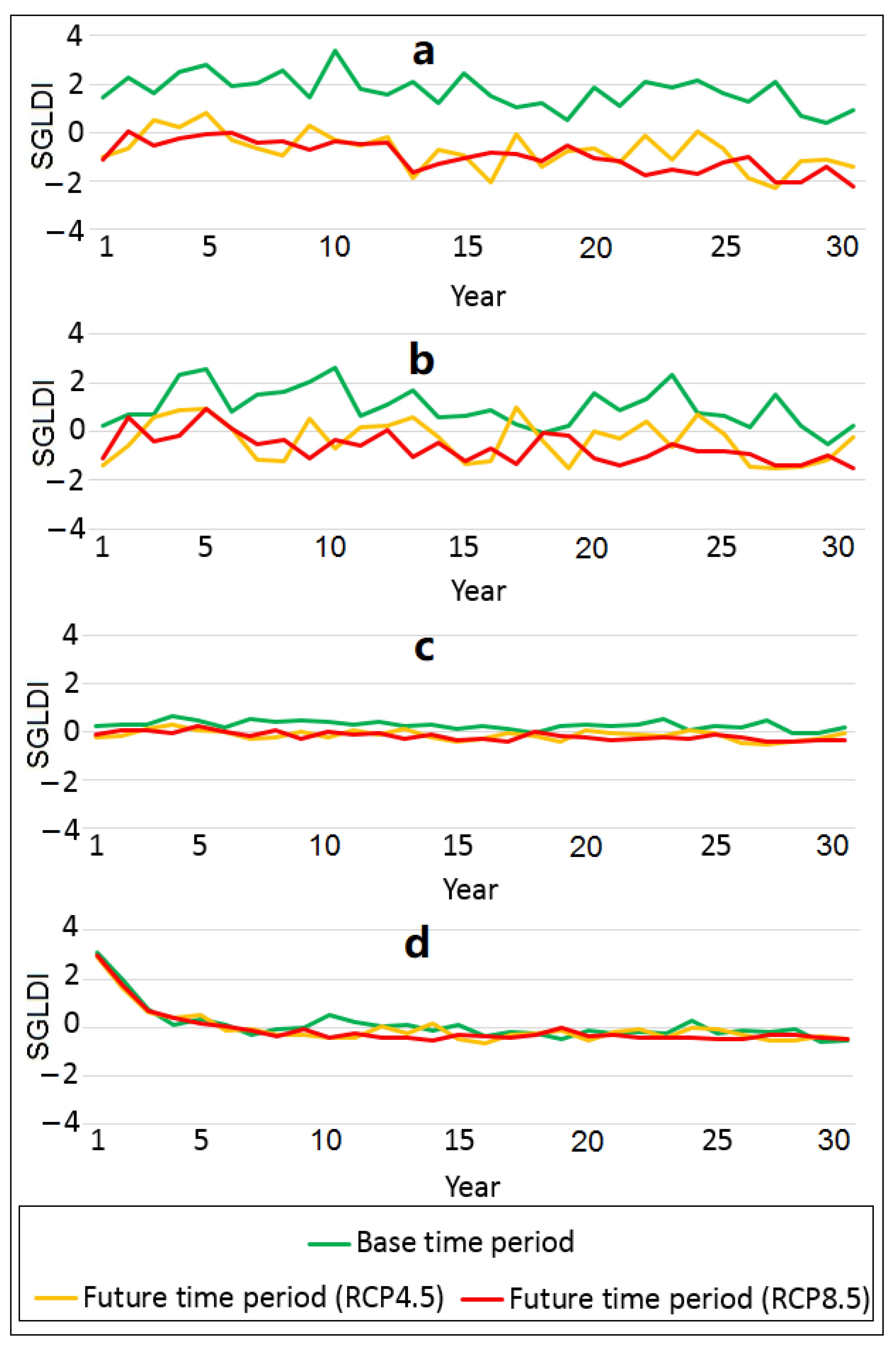
3.2.4. The SGLDI of the Karst Wells

Figure 6 and Table 4 illustrate the SGLDI values of the karst wells. With regard to W1, the curves of the future time period under RCP4.5 and RCP8.5 are very similar to each other and noticeably lower than the curve of the base time period (Figure 6a). For W3, all curves are parallel and they are quantitatively near zero (Figure 6c). Regarding W2, the intermediate situation of wells W1 and W3 is observed (Figure 6b).
In the base time period, the future time period under RCP4.5 and the future time period under RCP8.5, the mean SGLDI values are 1.72, −0.74 and −0.98 for W1, 1.01, −0.35 and −0.66 for W2 and 0.29, −0.12 and −0.16 for W3, all respectively (Table 4). In view of W1, a significant difference is observed between the future time period and the base time period. With respect to W2, a clear difference, even though less than W1, is also observed between the future time period and the base time period. The SGLDI values of the karst wells are smoother and virtually lower in the future time period under RCP8.5 than the future time period under RCP4.5 (Figure 6).
In view of the karst well W1, no year is observed with the unsatisfactory condition, i.e., with the SGLDI number of less than −1, in the base time period. The conditions are normal, relatively, very and extremely wet for this well in all years during the base time period. However, no year with relatively, very and extremely wet conditions is observed for this well in the future time period under RCP4.5. Seven years (2021, 2038, 2041, 2043, 2048, 2049 and 2050) with relatively dry, two years (2033 and 2046) with very dry and two years (2036 and 2047) with extremely dry conditions exist for this well in the future time period under RCP4.5 and the situation is normal for the rest of the years. The SGLDI values reduce from the beginning to the end of the future time period under RCP4.5. A maximum of five consecutive years, from 2046 to 2050, with a SGLDI of less than −1 is observed for this well in the future time period under RCP4.5. For this well, the situation would exacerbate in the future time period under RCP8.5 compared to the future time period under RCP4.5, such that there would be no relatively, very and extremely wet year in the future time period under RCP8.5. Regarding this well in the future time period under RCP8.5, nine years (2021, 2034, 2035, 2038, 2040, 2041, 2045, 2046 and 2049) with dry, four years (2033, 2042, 2043 and 2044) with very dry and three years (2047, 2048 and 2050) with extremely dry conditions exist and the situation is normal for the remaining years. For this well, the SGLDI values would decrease from the beginning to the end of the future time period under RCP8.5, as in the future time period under RCP4.5. A maximum of 11 consecutive years, from 2040 to 2050, with a SGLDI number of less than −1 are observed for this well in the future time period under RCP8.5 (Table 4). Generally, this well almost has low resilience to potential climate change.
In the case of the karst well W2, no year is observed with the unsatisfactory condition in the base time period, as in the case of the karst well W1. For W2 in the base time period, the conditions for all of the years are normal, relatively, very and extremely wet. However, for this well in the future time period under RCP4.5, only one year (2037) with a relatively wet condition is observed. Considering this well in the future time period under RCP4.5, eight years (2021, 2027, 2028, 2035, 2036, 2046, 2048 and 2049) with relatively dry and two years (2039 and 2047) with very dry conditions are observed and the situation is normal for the other years. As regards this well in the future time period under RCP4.5, dissimilar to W1, no year is observed with an extremely dry situation. Apropos of this well in the future time period under RCP4.5, the SGLDI values decline, especially in the last years, and a maximum of four consecutive years, from 2046 to 2049, with a SGLDI number of less than −1 exist. Regarding this well in the future time period under RCP8.5, there would be no relatively, very and extremely wet year, as in the future time period under RCP4.5. On the subject of this well in the future time period under RCP8.5, 10 years (2021, 2029, 2033, 2035, 2037, 2040, 2041, 2042, 2047 and 2048) with relatively dry and one year (2050) with very dry conditions exist and the situation is normal for the remaining years (Table 4). A maximum of three consecutive years, from 2040 to 2042, with a SGLDI number of less than −1 exist vis-à-vis this well in the future time period under RCP8.5 (Table 4). In general, this well presumably has a moderate resilience to potential climate change.
All years are in normal condition considering each period and scenario for the karst well W3. This indicates the high resilience of this well to potential climate change, which is forecasted to be higher than the Taraz-Harkesh stream, the Bibitarkhoun karst spring and two other karst wells. Indeed, no year with the unsatisfactory condition, i.e., with a SGLDI number of less than −1, is observed for W3 (Table 4).

3.2.5. The SGLDI of the Alluvial Aquifer

The SGLDI curves of the Pali alluvial aquifer (Figure 6d) are corresponding in each time period and emission scenario. The curves illustrate the highest SGLDI values in the first few years of each time period and emission scenario. In any case, they are like straight lines overlapping each other if the first few years are excluded.
The mean SGLDI values of the Pali alluvial aquifer (Table 4) are 0.11, −0.03 and −0.08 in the base time period, the future time period under RCP4.5 and the future time period under RCP8.5, respectively. In each time period and emission scenario, very and extremely wet conditions are anticipated for the first two years and the situation is normal for the other years. Moreover, relatively, very and extremely dry conditions are not predicted for the aquifer in every time period and emission scenario. Therefore, the Pali alluvial aquifer is the most resilient water resource in the Lali region towards potential climate change.

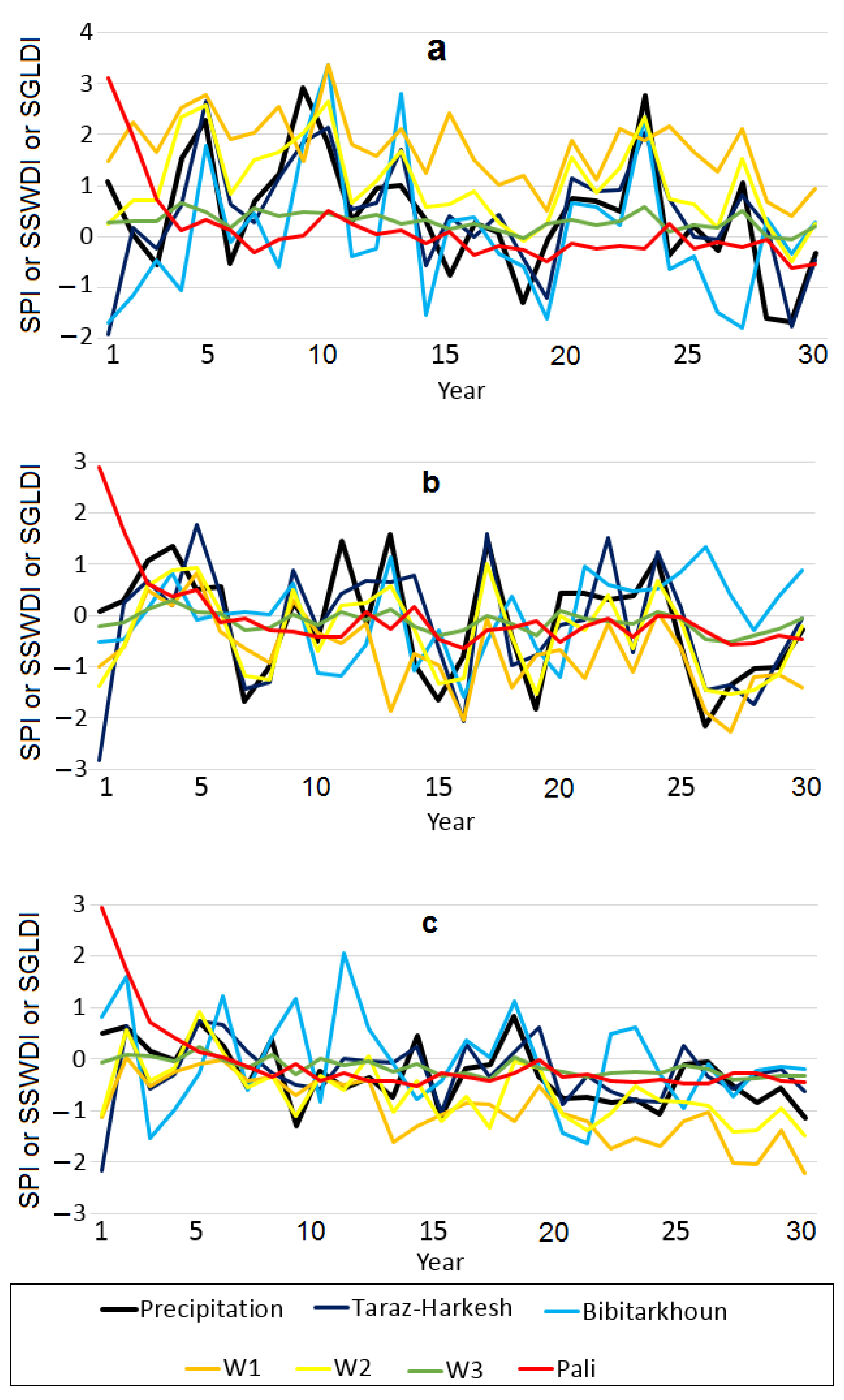
3.2.6. Comparison between the SPI, SSWDI and SGLDI Values

The SGLDI and SSWDI curves almost follow the trend of the SPI curves for different water resources of the Lali region in the base (Figure 7a), the future under RCP4.5 (Figure 7b) and the future under RCP8.5 (Figure 7c) time periods. In every time period and emission scenario, the SGLDI of the Pali alluvial aquifer and the SSWDI of the Taraz-Harkesh stream have the lowest and the highest correlations with the SPI, respectively (Figure 7). Even though the SGLDI curves of the wells W1 and W2 are approximately higher than the SPI curve in the base time period and lower than the SPI curves in the future time period, considering both emission scenarios, they virtually follow the trend of the SPI curves. The resilient characteristics of the Pali alluvial aquifer and W3 to potential climate change are fairly similar so that their curves almost follow the same trend. Finally, the SGLDI of the Bibitarkhoun karst spring follows the trend of the SPI, especially in the base time period.

3.3. Quantification of the GRI and SWRI of Water Resources

Subsequent to computing the SGLDI and SSWDI of the water resources in the Lali region in different years in the base and future time periods under RCP4.5 and RCP8.5, their resilience, i.e., GRI and SWRI, were quantitatively calculated as a number between zero and one (Table 5). The GRI of the Pali alluvial aquifer and W3 is one, considering each method, time period and emission scenario. Moreover, the total average SWRI is 0.79, 0.6, 0.59 and 0.52 for the Taraz-Harkesh stream, W2, the Bibitarkhoun spring and W1, respectively (Table 5).
The mean GRI and SWRI values acquired from the methods 1 and 2 almost correspond to the total average illustrating that the Pali alluvial aquifer, W3, the Taraz-Harkesh stream, W2, the Bibitarkhoun spring and W1 follow the trend in which resilience to climate change declines. As regards method 3, the calculated total average of the GRI and SWRI is not dissimilar to other methods for different water resources, except that the GRI of the Bibitarkhoun karst spring is more than W2. Additionally, the calculated values of the average GRI and SWRI have the least variation in method 3.
GRI diminishes from the base time period to the future time period under RCP8.5, with the future time period under RCP4.5 at the intermediate level, for W1, regarding all methods and the total average. The same trend is observed for W2, excluding method 2. The equivalent situation is not observed for the Taraz-Harkesh stream and the Bibitarkhoun karst spring. In other words, if GRI is considered in the future time period under RCP4.5 and RCP8.5 in comparison with the base time period, it can be construed that the GRI values of W1 and W2 have a more marked decline in the future time period than those in the base time period. Furthermore, their GRI is slightly higher in the future time period under RCP4.5 than that in the future time period under RCP8.5 (Table 5).

4. Discussion

In regard to the impacts of geological and geomorphological characteristics on the climate in the Lali region, it may be mentioned that the precipitation pattern in the region does not clearly follow local factors such as topography, as heavy precipitation of Sudanese systems with convective motions occur over the region with high spatio-temporal variabilities [54].
It is vital to assess the impact of climate change on groundwater recharge and discharge rates [39]. Storm events with intense precipitation are expected to escalate the situation as energy increases in the climate system [83,84]. Moreover, the time of monsoon precipitation may also change, resulting in amplified groundwater demand. Therefore, proposing the SPI methodology to assess the groundwater resilience may be of high significance.
Lapworth et al. [41] examined groundwater resilience to potential climate change in West Africa. Results revealed that shallow groundwater is primarily recharged subsequent to precipitation at a rapid rate. In other words, little evidence of evaporation exists prior to groundwater recharge. In arid areas with precipitation less than 400 mm/year, groundwater recharge may be roughly up to 20 mm/year. These indicate high resilience of water resources to short-term (inter-annual) precipitation and groundwater recharge variations so that any future changes in precipitation and groundwater recharge due to climate change are unlikely to cause failure in the groundwater supplies on the continental scale. In the current study, which is a local-scale case study, climate change cannot lead to failure in the Pali alluvial aquifer and the karst well W3. However, failure probably occurs in the case of the karst wells W1 and W2, even if only climate change is regarded.
Davidson [40] employed aquifer resilience as an inherent capacity of the aquifer to maintain groundwater reserves and groundwater balance components during the drought conditions. It was concluded that large unconfined aquifers have high resilience and confined aquifers discharging trifling volumes of water have low resilience. Principally, the main aquifers of Marlborough were divided into three categories, regarding groundwater resilience, as follows:
1-
High resilience: if groundwater uniformly supplies the river’s base flow over time, it has high resilience. These aquifers contain large storage of groundwater.
2-
Moderate resilience: if groundwater relatively variably provides the river’s base flow over time, it has moderate resilience. These aquifers contain moderate storage of groundwater.
3-
Low resilience: if groundwater very variably feeds the river’s base flow over time through the springs, it has low resilience. These aquifers contain low storage of groundwater.
MacDonald et al. [39] examined the groundwater resources in the Indo-Gangetic Basin, emphasizing their resilience to climate change and groundwater abstraction. They declared that a diminutive decrement in the groundwater level can influence the aquatic ecosystem, the stream flow and the discharge of the shallow wells. As a result, considering the uncertainty of precipitation and the possibility of continuous increment in the groundwater discharge in the future time period, the best approach is to assess the resilience of groundwater resources to these two factors, namely climate change and groundwater abstraction. Groundwater demonstrates a decade-old age in Nepal, indicating the aquifer resilience to the annual changes in precipitation. Even though most springs are not resilient to climate change, they would probably discharge small flows during droughts.
MacDonald et al. [38] proposed two scenarios regarding groundwater resilience. The first scenario is the resilience of groundwater resources to short-term climatic stresses (less than a year). This scenario is affected by the availability of the groundwater storage as well as the average long-term (decadal) groundwater recharge [85]. Therefore, in a thin hard-rock aquifer with aerated layers, subsequent to several years of drought, groundwater returns to the previous (satisfactory) condition more quickly if the system has a high long-term recharge than if it has a low long-term recharge [86]. The second scenario is the resilience of groundwater resources to long-term (decadal) climate change. This scenario is based on the available groundwater storage. Climate change affects the larger groundwater systems less than the smaller ones. In the current study, in which the aquifers are small-scale, the karst wells W1 and W2 illustrate low resilience to climate change, considering the second scenario. However, other water resources, especially the Pali alluvial aquifer and the karst well W3, show high resilience to climate change. Accordingly, depending on the hydrogeological characteristics, aquifers of the same scale may exhibit different behaviour towards climate change with respect to the second scenario.
As previously mentioned, the high resilience of the Taraz-Harkesh stream is possibly due to the fact that it has a high base flow due to being recharged by the Pali alluvial aquifer, which is the most resilient resource of water to climate change in the Lali region.
Hydrogeologically, wells are expected to have more resilience than springs. Regarding the water resources of the Lali region, the karst well W3, which is the closest well to the Bibitarkhoun karst spring, has average GRI of one and the Bibitarkhoun karst spring has average GRI of 0.59. The GRI values of the well W2 and the Bibitarkhoun karst spring are similar and higher than that of the karst well W1. The karst well W1 has the least GRI to climate change, perhaps due to its location at the upstream or feeding area of the Asmari karst aquifer (Figure 1). Wells W1, W2 and W3 are directed from the recharge zone to the discharge zone of the karst aquifer. Resilience of the wells increases from the upstream to the downstream areas (close to the base level of erosion) of the aquifer.

5. Advantages and Disadvantages of the Employed Methodology

One of the advantages of utilising the SPI approach to study the resilience of water resources is that precipitation and its variations can be taken into consideration alongside the changes in groundwater resources. Additionally, the method does not entail much data. In the current study, solely data on precipitation, groundwater level and the discharge rate of springs or streams are required. These data have been attained for the Lali region even for the base (1961–1990) and future (2021–2050) time periods by simulation. The method can be used in local case studies even at the scale of a well or a spring. It can be applied to surface water alongside alluvial, karst and hard-rock aquifers. Moreover, according to the proposed methods, resilience index can be computed as a number between zero and one and, as a result, different water resources can be compared. Indeed, the operational criteria can be normalized by considering the minimum and maximum values so that the groundwater GRI of different aquifers can be quantitatively computed [46]. This is opposite to most other studies, which have assessed the groundwater resilience only qualitatively, e.g., [53].
One significant issue in the context of resilience is the failure threshold or the occurrence of unsatisfactory condition. Unfortunately, it is still not obvious how the threshold of failure is quantified for an aquifer. Diminution in the long-term storage is the aquifer resilience limit, indicating the inability of the aquifer to maintain equilibrium in the presence of unsatisfactory condition [30]. Thomas et al. [46] considered the negative values as the unsatisfactory condition and the positive values as the satisfactory condition after determining the Grace-Groundwater Drought Index (GGDI) and normalizing it. One of the benefits of the current study is that the failure threshold can be pinpointed as relatively, very and extremely dry conditions with the SGLDI and SSWDI values of less than −1, −1.5 and −2, respectively. Should the failure threshold be exceeded, an unsatisfactory condition occurs. On the other hand, Peterson and Western [37] remarked that a system may have several steady states instead of one steady state. In the current study, according to the SGLDI and SSWDI values, different conditions, from extremely wet to extremely dry, have been considered. However, the results of the current study have been produced concerning the groundwater level fluctuations and discharge rates.
Groundwater storage is a significant factor in defining the groundwater resilience. Despite the fact that the Pali alluvial aquifer probably has the highest resilience to climate change, its storage is low, being a small-scale aquifer. Furthermore, in the case of the Asmari karst aquifer, the resilience increases from the recharge area to the discharge area. Conclusively, all hydrogeological factors should be concerned in the study of water resources resilience. Moreover, quantifying the resilience is not undemanding considering the groundwater storage due to the complexity of estimation. However, the uncertainty associated with the groundwater storage restricts the determination of the aquifer resilience [30]. Zeydalinejad et al. [52] studied the resilience of the Bibitarkhoun karst spring utilising the gamma distribution in the base (1961–1990) and future (2021–2050) time periods concerning the discharge rates and dynamic storages of the spring. The latter was computed using the loss curves. The results exhibited that the resilience quantified by the discharge rates of the spring is probably more accurate than the one calculated by the dynamic storages of the spring. The reason might be the logarithmic nature of the method used to determine the dynamic storages of the spring. In any event, it is recommended that all factors other than climate change be considered if they influence the system.
Finally, Chinnasamy et al. [48] confirmed that there are limitations to utilising the SPI method in determining aquifer resilience. This method is sensitive to data quality, sample size or data length and the employed normalizing approach. In addition, this method cannot be used for areas with low seasonal rainfall and short time series and it only considers one variable at a time. Hence, it assumes that the considered variable is independent of other processes.

6. Conclusions

As was explained, the concept of resilience has not frequently been employed in the groundwater literature. Most studies assessing groundwater resilience have been published during recent years. Various indices used in groundwater, including resilience, have mainly been applied in drought and managerial perspectives [87,88,89,90,91,92,93,94,95,96]. However, utilising the operational criteria, e.g., resilience, can be considered as a practical concept in the groundwater studies, e.g., 56 and 60. In the current study, making use of the SGLDI, SSWDI and SPI concepts has been proposed to calculate the groundwater resilience of different water systems to potential climate change. The approach was able to compare the resilience of different water systems during different years under the emission scenarios.
The GRI values of the Pali alluvial aquifer and the karst well W3 to the future climate change were determined to be one. Moreover, the average resilience index is 0.79, 0.6, 0.59 and 0.52 for the Taraz-Harkesh stream, the karst well W2, the Bibitarkhoun karst spring and the karst well W1, respectively. The Taraz-Harkesh stream, which has a very high base flow and is recharged by the alluvial aquifer, has a relatively high resilience. In addition to being fed from the alluvial aquifer, this stream may also be recharged from the karst aquifer of the Asmari Formation. Moreover, the Bibitarkhoun karst spring has a comparative high resilience to future climate change, which is due to the fact that it is a permanent, and the largest, spring in the study area. This spring is considered as the base-level of the karst aquifer in the study area. The karst well W1, which is located at the upstream or recharge zone of the Asmari karst aquifer, has the lowest resilience, so that its resilience is even less than that of the Bibitarkhoun karst spring. The karst wells W1, W2 and W3 are, respectively, located from the recharge zone to the discharge area of the aquifer and their resilience follows the same trend. Indeed, climate change may have diminutive influence on the alluvial aquifers and streams recharged by groundwater or having high base flows. On the other hand, climate change may have a significant impact on surface waters with low base flows. However, the behaviour of karst aquifers with respect to climate change may be similar to alluvial aquifers with high storages (high resilience) or surface waters with low base flows (low resilience). In other words, the resilience of karst aquifers to the future climate change is more ambiguous. Therefore, studying the impact of climate change on karst aquifers is definitely recommended.
The results of this study show that considering the groundwater storage alone as the measure of aquifer resilience may be misleading. The Lali region is a small-scale and sub-basin area with different water resources in which not only do different water resources have dissimilar resilience to climate change, but the water resources of one aquifer, i.e., the karst aquifer of the Asmari Formation, also behave differently towards climate change.
Finally, this study demonstrated that the karstic aquifers may have more ambiguous response towards the potential climate change in comparison with the alluvial aquifer and surface water. Indeed, the influence of geological and structural settings of a karstic terrain is of paramount significance, as also declared by [97]. Therefore, it is highly recommended that the hydrogeological properties of the Asmari karstic aquifer be studied in detail in the Lali region to specify the spatial heterogeneities and characteristics of the aquifer.

Author Contributions

Conceptualization, N.Z., H.R.N., F.A., A.S. and B.G.; Data curation, N.Z., H.R.N., F.A., A.S. and B.G.; Formal analysis, N.Z., H.R.N., F.A., A.S. and B.G.; Funding acquisition, N.Z.; Investigation, N.Z., H.R.N., F.A. and A.S.; Methodology, N.Z., H.R.N., A.S. and B.G.; Project administration, H.R.N.; Resources, N.Z. and H.R.N.; Software, N.Z.; Supervision, N.Z. and H.R.N.; Validation, N.Z., H.R.N., A.S. and B.G.; Visualization, N.Z., H.R.N., F.A. and A.S.; Writing—original draft, N.Z.; Writing—review & editing, H.R.N., F.A., A.S. and B.G. All authors have read and agreed to the published version of the manuscript.

Funding

This research received no external funding.

Data Availability Statement

Not applicable.

Conflicts of Interest

The authors declare no conflict of interest.

References

  1. Shiklomanov, I.A. World freshwater resources. In Water in Crisis: A Guide to the World’s Fresh Water Resources; Gleick, P.H., Ed.; Oxford University Press: New York, NY, USA, 1993; pp. 13–24. [Google Scholar]
  2. Grönwall, J.; Oduro-Kwarteng, S. Groundwater as a strategic resource for improved resilience: A case study from peri urban Accra. Environ. Earth Sci. 2018, 77, 6. [Google Scholar] [CrossRef] [Green Version]
  3. Zeydalinejad, N.; Nassery, H.R.; A review on the climate-induced depletion of Iran’s aquifers. Stoch. Environ. Res. Risk. Assess. 2022. Available online: https://link.springer.com/article/10.1007/s00477-022-02278-z (accessed on 1 November 2019).
  4. Ghazi, B.; Jeihouni, E.; Kouzehgar, K.; Torabi Haghighi, A. Assessment of probable groundwater changes under representative concentration pathway (RCP) scenarios through the wavelet–GEP model. Environ. Earth Sci. 2021, 80, 446. [Google Scholar] [CrossRef]
  5. Ghazi, B.; Jeihouni, E.; Kisi, O.; Pham, Q.B.; Durin, B. Estimation of Tasuj aquifer response to main meteorological parameter variations under Shared Socioeconomic Pathways scenarios. Theor. Appl. Climatol. 2022, 149, 25–37. [Google Scholar] [CrossRef]
  6. Hashimoto, T.; Stedinger, J.R.; Loucks, D.P. Reliability, resiliency, and vulnerability criteria for water resource system performance evaluation. Water Resour. Res. 1982, 18, 14–20. [Google Scholar] [CrossRef] [Green Version]
  7. Holling, C.S. Resilience and stability of ecological systems. Annu. Rev. Ecol. Syst. 1973, 4, 1–23. [Google Scholar] [CrossRef] [Green Version]
  8. Roach, T.; Kapelan, Z.; Ledbetter, R. A resilience-based methodology for improved water resources adaptation planning under deep uncertainty with real world application. Water Resour. Manag. 2018, 32, 2013–2031. [Google Scholar] [CrossRef] [Green Version]
  9. Grey, D.; Sadoff, C. Sink or swim? water security for growth and development. Water Policy 2007, 9, 545–571. [Google Scholar] [CrossRef]
  10. Ait-Kadi, M.; Lincklaen-Arriens, W. Increasing Water Security: A Development Imperative; Global Water Partnership (GWP): Stockholm, Sweden, 2012. [Google Scholar]
  11. Foster, S.; MacDonald, A. The water security dialogue: Why it needs to be better informed about groundwater. Hydrogeol. J. 2014, 22, 1489–1492. [Google Scholar] [CrossRef]
  12. Vaz, A.C. Reliability in water resources planning. In Systems Analysis Applied to Water and Related Land Resources; Valadares Tavares, L., Evaristo Da Silva, J., Eds.; Pergamon Press: Tarrytown, NY, USA, 1986. [Google Scholar]
  13. Maier, H.R.; Lence, B.J.; Tolson, B.A.; Foschi, R.O. First-order reliability method for estimating reliability, vulnerability and resilience. Water Resour. Res. 2001, 37, 779–790. [Google Scholar] [CrossRef] [Green Version]
  14. Loucks, D.P. Quantifying trends in system sustainability. Hydrol. Sci. J. 1997, 42, 513–530. [Google Scholar] [CrossRef]
  15. Loucks, D.P.; Van Beek, E.; Stedinger, J.R.; Dijkman, J.P.; Villars, M.T. Water Resources Systems Planning and Management: An Introduction to Methods, Models and Applications; UNESCO: Paris, France, 2005. [Google Scholar]
  16. Kjeldsen, T.R.; Rosbjerg, D. A framework for assessing the sustainability of a water resources system. In Regional Management of Water Resources; Schumann, A., Ed.; IAHS Publication: Maastricht, The Netherlands, 2001; pp. 107–113. [Google Scholar]
  17. McMahon, T.A.; Adeloye, A.J.; Zhou, S.L. Understanding performance measures of reservoirs. J. Hydrol. 2006, 324, 359–382. [Google Scholar] [CrossRef]
  18. Moy, W.S.; Cohon, J.L.; ReVelle, C.S. A programming model for analysis of the reliability, resilience and vulnerability of a water supply reservoir. Water Resour. Res. 1986, 22, 489–498. [Google Scholar] [CrossRef]
  19. Mendoza, V.M.; Villanueva, E.E.; Adem, J. Vulnerability of basins and watersheds in Mexico to global climate change. Clim. Res. 1997, 9, 139–145. [Google Scholar] [CrossRef] [Green Version]
  20. Nelson, D. Adaptation and resilience: Responding to a changing climate. Wiley Interdiscip. Rev. Clim. Chang. 2011, 2, 113–120. [Google Scholar] [CrossRef]
  21. Barbieri, M.; Barberio, M.D.; Banzato, F.; Billi, A.; Boschetti, T.; Franchini, S.; Gori, F.; Petitta, M. Climate change and its effect on groundwater quality. Environ. Geochem. Health 2021, 1–12. [Google Scholar] [CrossRef]
  22. Barbieri, M.; Ricolfi, L.; Vitale, S.; Muteto, P.V.; Nigro, A.; Sappa, G. Assessment of groundwater quality in the buffer zone of Limpopo National Park, Gaza Province, Southern Mozambique. Environ. Sci. Pollut. Res. 2019, 26, 62–77. [Google Scholar] [CrossRef]
  23. Ricolfi, L.; Barbieri, M.; Muteto, P.V.; Nigro, A.; Sappa, G.; Vitale, S. Potential toxic elements in groundwater and their health risk assessment in drinking water of Limpopo National Park, Gaza Province, Southern Mozambique. Environ. Geochem. Health 2020, 42, 2733–2745. [Google Scholar] [CrossRef]
  24. Hera-Portillo, A.D.L.; Lopez-Gutierrez, J.; Zorrilla-Miras, P.; Mayor, B.; Lopez-Gunn, E. The ecosystem resilience concept applied to hydrogeological systems: A general approach. Water 2020, 12, 1824. [Google Scholar] [CrossRef]
  25. Sharma, U.C.; Sharma, V. Groundwater sustainability indicators for the Brahmaputra basin in the northeastern region of India. In Sustainability of Groundwater Resources and Its Indicators; Webb, B., Ed.; IAHS Press: Foz do Iguacu, Brazil, 2006; pp. 43–50. [Google Scholar]
  26. Shrestha, S.; Neupanea, S.; Mohanasundarama, S.; Pandey, V.P. Mapping groundwater resiliency under climate change scenarios: A case study of Kathmandu Valley, Nepal. Environ. Res. 2020, 183, 109149. [Google Scholar] [CrossRef]
  27. Steijn, T.V.; Verhagen, F.; Hunink, J. Quantifying groundwater resilience in Noord-Brabant, the Netherlands. Geophys. Res. Abstr. 2018, 20, 8448. [Google Scholar]
  28. Kumar, N.; Sinha, J.; Madramootoo, C.A.; Goyal, M.K. Quantifying groundwater sensitivity and resilience over peninsular India. Hydrol. Process. 2020, 34, 5327–5339. [Google Scholar] [CrossRef]
  29. UN World Water Assessment Program (WWAP). Water for People-Water for Life; UNESCO Publication: Barcelona, Spain, 2003. [Google Scholar]
  30. Richey, A.S.; Thomas, B.F.; Lo, M.H.; Famiglietti, J.S.; Swenson, S.; Rodell, M. Uncertainty in global groundwater storage estimates in a Total Groundwater Stress framework. Water Resour. Res. 2015, 51, 5198–5216. [Google Scholar] [CrossRef] [PubMed]
  31. Katic, P.; Grafton, R.Q. Optimal groundwater extraction under uncertainty: Resilience versus economic payoffs. J. Hydrol. 2011, 406, 215–224. [Google Scholar] [CrossRef]
  32. Herrera-Franco, G.; Carrion-Mero, P.; Aguilar-Aguilar, M.; Morante-Carballo, F.; Jaya-Montalvo, M.; Morillo Balsera, M.C. Groundwater Resilience Assessment in a Communal Coastal Aquifer System. The Case of Manglaralto in Santa Elena, Ecuador. Sustainability 2020, 12, 8290. [Google Scholar] [CrossRef]
  33. Hund, S.V.; Allen, D.M.; Morillas, L.; Johnson, M.S. Groundwater recharge indicator as tool for decision makers to increase socio-hydrological resilience to seasonal drought. J. Hydrol. 2018, 563, 1119–1134. [Google Scholar] [CrossRef]
  34. Peters, E.; van Lanen, H.A.J.; Torfs, P.J.J.F.; Bier, G. Drought in groundwater- drought distribution and performance indicators. J. Hydrol. 2005, 306, 302–317. [Google Scholar] [CrossRef]
  35. Peterson, T.J.; Argent, R.M.; Western, A.W.; Chiew, F.H.S. Multiple stable states in hydrological models: An ecohydrological investigation. Water Resour. Res. 2009, 45, W03406. [Google Scholar] [CrossRef]
  36. Peterson, T.J.; Western, A.W. Multiple hydrological attractors under stochastic daily forcing: Can multiple attractors exist? Water Resour. Res. 2014, 50, 2993–3009. [Google Scholar] [CrossRef]
  37. Peterson, T.; Western, A.; Argent, R. Analytical methods for ecosystem resilience: A hydrological investigation. Water Resour. Res. 2012, 48, 1–16. [Google Scholar] [CrossRef]
  38. MacDonald, A.M.; Bonsor, H.C.; Calow, R.C.; Taylor, R.G.; Lapworth, D.J.; Maurice, L.; Tucker, J.; O Dochartaigh, B.E. Groundwater Resilience to Climate Change in Africa, Open Report OR/11/031; British Geological Survey: Nottingham, UK, 2011. [Google Scholar]
  39. MacDonald, A.M.; Bonsor, H.C.; Taylor, R.G.; Shamsudduha, M.; Burgess, W.G.; Ahmed, K.M.; Mukherjee, A.; Zahid, A.; Lapworth, D.; Krishan, G.; et al. Groundwater Resources in the Indo-Gangetic Basin: Resilience to Climate Change and Abstraction; British Geological Survey: Nottingham, UK, 2015. [Google Scholar]
  40. Davidson, P. Aquifer Dynamics and Resilience Review, MDC Technical Report No: 12-001; Marlborough District Council: Marlborough, UK, 2012. [Google Scholar]
  41. Lapworth, D.J.; MacDonald, A.M.; Tijani, M.N.; Darling, W.G.; Gooddy, D.C.; Bonsor, H.C.; Araguás-Araguás, L.J. Residence times of shallow groundwater in West Africa: Implications for hydrogeology and resilience to future changes in climate. Hydrogeol. J. 2013, 21, 673–686. [Google Scholar] [CrossRef] [Green Version]
  42. Richey, A.S. Stress and Resilience in the World’s Largest Aquifer Systems: A GRACE-Based Methodology. Ph.D. Dissertation, University of California, Los Angeles, CA, USA, 2014. [Google Scholar]
  43. Alraggad, M.; Johnsen-Harris, B.; Shdaifat, A.; Abugazleh, M.K.; Hamaideh, A. Groundwater resilience to climate change in the eastern Dead Sea basin- Jordan. Sci. Res. Essays 2017, 12, 24–41. [Google Scholar]
  44. Kamali, A.; Niksokhan, M.H. Multi-objective optimization for sustainable groundwater management by developing of coupled quantity-quality simulation-optimization model. J. Hydroinform. 2017, 19, 973–992. [Google Scholar] [CrossRef]
  45. Thomas, B.F. Sustainability indices to evaluate groundwater adaptive management: A case study in California (USA) for the Sustainable Groundwater Management Act. Hydrogeol. J. 2019, 27, 239–248. [Google Scholar] [CrossRef]
  46. Thomas, B.F.; Caineta, J.; Nanteza, J. Global assessment of groundwater sustainability based on storage anomalies. Geophys. Res. Lett. 2017, 44, 445–455. [Google Scholar] [CrossRef] [Green Version]
  47. Al-Amin, S.; Berglund, E.Z.; Mahinthakumar, G.; Larson, K.L. Assessing the effects of water restrictions on socio-hydrologic resilience for shared groundwater systems. J. Hydrol. 2018, 566, 872–885. [Google Scholar] [CrossRef]
  48. Chinnasamy, P.; Maheshwari, B.; Prathapar, S.A. Adaptation of standardised precipitation index for understanding water table fluctuations and groundwater resilience in hard-rock areas of India. Environ. Earth Sci. 2018, 77, 562. [Google Scholar] [CrossRef]
  49. Fuchs, E.H.; Carroll, K.C.; King, J.P. Quantifying groundwater resilience through conjunctive use for irrigated agriculture in a constrained aquifer system. J. Hydrol. 2018, 565, 747–759. [Google Scholar] [CrossRef]
  50. Wurl, J.; Gámez, A.E.; Ivanova, A.; Lamadrid, M.A.I.; Morales, P.H. Socio-hydrological resilience of an arid aquifer system, subject to changing climate and inadequate agricultural management: A case study from the Valley of Santo Domingo, Mexico. J. Hydrol. 2018, 559, 486–498. [Google Scholar] [CrossRef]
  51. Niyazi, B.A.; Ahmed, M.; Masoud, M.Z.; Rashed, M.A.; Basahi, J.M. Sustainable and resilient management scenarios for groundwater resources of the Red Sea coastal aquifers. Sci. Total Environ. 2019, 690, 1310–1320. [Google Scholar] [CrossRef]
  52. Zeydalinejad, N.; Nassery, H.R.; Alijani, F.; Shakiba, A. Forecasting the resilience of Bibitarkhoun karst spring, southwest Iran, to the future climate change. Model. Earth Syst. Environ. 2020, 6, 2359–2375. [Google Scholar] [CrossRef]
  53. Nassery, H.R.; Zeydalinejad, N.; Alijani, F. Speculation on the resilience of karst aquifers using geophysical and GIS-based approaches (a case study of Iran). Acta Geophys. 2021, 69, 2393–2415. [Google Scholar] [CrossRef]
  54. Zeydalinejad, N.; Nassery, H.R.; Shakiba, A.; Alijani, F. Prediction of the karstic spring flow rates under climate change by climatic variables based on the artificial neural network: A case study of Iran. Environ. Monit. Assess. 2020, 192, 375. [Google Scholar] [CrossRef] [PubMed]
  55. Nassery, H.R.; Zeydalinejad, N.; Alijani, F.; Shakiba, A. A proposed modelling towards the potential impacts of climate change on a semi-arid, small-scaled aquifer: A case study of Iran. Environ. Monit. Assess. 2021, 193, 182. [Google Scholar] [CrossRef] [PubMed]
  56. Mazi, K.; Koussis, A.D.; Destouni, G. Intensively exploited Mediterranean aquifers: Resilience to seawater intrusion and proximity to critical thresholds. Hydrol. Earth Syst. Sci. 2014, 18, 1663–1677. [Google Scholar] [CrossRef] [Green Version]
  57. Zhang, Y.; Wang, Y.; Chen, Y.; Liang, F.; Liu, H. Assessment of future flash flood inundations in coastal regions under climate change scenarios-A case study of Hadahe River basin in northeastern China. Sci. Total Environ. 2019, 693, 133550. [Google Scholar] [CrossRef]
  58. Sajjad, H.; Ghaffar, A. Observed, simulated and projected extreme climate indices over Pakistan in changing climate. Theor. Appl. Climatol. 2018, 137, 255–281. [Google Scholar] [CrossRef]
  59. Sahany, S.; Mishra, S.K.; Salunke, P. Historical simulations and climate change projections over India by NCAR CCSM4: CMIP5 vs. NEX-GDDP. Theor. Appl. Climatol. 2018, 135, 1423–1433. [Google Scholar] [CrossRef]
  60. Cao, F.; Gao, T. Effect of climate change on the centennial drought over China using high-resolution NASA-NEX downscaled climate ensemble data. Theor. Appl. Climatol. 2019, 138, 1189–1202. [Google Scholar] [CrossRef]
  61. Thrasher, B.; Maurer, E.P.; McKellar, C.; Duffy, P.B. Technical note: Bias correcting climate model simulated daily temperature extremes with quantile mapping. Hydrol. Earth Syst. Sci. 2012, 16, 3309–3314. [Google Scholar] [CrossRef] [Green Version]
  62. Wood, A.W.; Leung, L.R.; Sridhar, V.; Lettenmaier, D.P. Hydrologic implications of dynamical and statistical approaches to downscaling climate model outputs. Clim. Chang. 2004, 62, 189–216. [Google Scholar] [CrossRef]
  63. Wood, A.W.; Maurer, E.P.; Kumar, A.; Lettenmaier, D.P. Long-range experimental hydrologic forecasting for the eastern United States. J. Geophys. Res. 2002, 107, 4429. [Google Scholar] [CrossRef]
  64. Stackhouse, P.W.; Gupta, S.K.; Cox, S.J.; Mikowitz, J.C.; Zhang, T.; Chiacchio, M. 12-year surface radiation budget data set. GEWEX News 2004, 14, 10–12. [Google Scholar]
  65. Maurer, E.P.; Hidalgo, H.G. Utility of daily vs. monthly large-scale climate data: An intercomparison of two statistical downscaling methods. Hydrol. Earth Syst. Sci. 2008, 12, 551–563. [Google Scholar] [CrossRef]
  66. Bokhari, S.A.A.; Ahmad, B.; Ali, J.; Ahmad, S.; Mushtaq, H.; Rasul, G. Future climate change projections of the Kabul River Basin using a multi model ensemble of high resolution statistically downscaled data. Earth Syst. Environ. 2018, 2, 477–497. [Google Scholar] [CrossRef]
  67. Jain, S.; Salunke, P.; Mishra, S.K.; Sahany, S.; Choudhary, N. Advantage of NEX-GDDP over CMIP5 and CORDEX Data: Indian Summer Monsoon. Atmos. Res. 2019, 228, 152–160. [Google Scholar] [CrossRef]
  68. Singh, V.; Jain, S.K.; Singh, P.K. Inter-comparisons and applicability of CMIP5 GCMs, RCMs and statistically downscaled NEX-GDDP based precipitation in India. Sci. Total Environ. 2019, 697, 134163. [Google Scholar] [CrossRef]
  69. Zeydalinejad, N.; Nassery, H.R.; Shakiba, A.; Alijani, F. The evaluations of NEX-GDDP and Marksim downscaled datasets over Lali region, southwest Iran. J. Earth Space Phys. 2021, 46, 213–230. [Google Scholar] [CrossRef]
  70. Zeydalinejad, N.; Nassery, H.R.; Shakiba, A.; Alijani, F. Simulation of Taraz-Harkesh river’s fow, Khouzestan Province, under climate change with NEX-GDDP data set and IHACRES rainfall-runoff model. J. Meteorol. Atmos. Sci. 2019, 2, 162–178. (In Persian) [Google Scholar]
  71. Roushangar, K.; Alizadeh, F.; Nourani, V. Improving capability of conceptual modeling of watershed rainfall–runoff using hybrid wavelet-extreme learning machine approach. J. Hydroinform. 2018, 20, 69–87. (In Persian) [Google Scholar] [CrossRef] [Green Version]
  72. Zeydalinejad, N.; Nassery, H.R.; Shakiba, A.; Alijani, F. Simulation of karst aquifer water level under climate change in Lali region, Khouzestan Province, SW Iran. Nivar 2020, 44, 97–109. (In Persian) [Google Scholar] [CrossRef]
  73. McKee, T.B.; Doesken, N.J.; Kleist, J. The Relationship of Drought Frequency and Duration to Time Scales. In Proceedings of the 8th Conference on Applied Climatology, American Meteorological Society, Boston, MA, USA, 17–22 January 1993. [Google Scholar]
  74. Edwards, D.C.; McKee, T.B. Characteristics of 20th Century Drought in the United States at Multiple Time Scales; Colorado State University: Fort Collins, CO, USA, 1997. [Google Scholar]
  75. WMO. Standardized Precipitation Index-User Guide; World Meteorological Organization: Geneva, Switzerland, 2012. [Google Scholar]
  76. Vasiliades, L.; Loukas, A.; Liberis, N. A water balance derived drought index for Pinios river basin, Greece. Water Resour. Manag. 2011, 25, 1087–1101. [Google Scholar] [CrossRef]
  77. Shukla, S.; Wood, A.W. Use of a standardized runoff index for characterizing hydrologic drought. Geophys. Res. Lett. 2008, 35, 1–7. [Google Scholar] [CrossRef] [Green Version]
  78. Angelidis, P.; Maris, F.; Kotsovinos, N.; Hrissanthou, V. Computation of drought index SPI with alternative distribution functions. Water Resour. Manag. 2012, 26, 2453–2473. [Google Scholar] [CrossRef]
  79. Tigkas, D.; Vangelis, H.; Tsakiris, G. DrinC: A software for drought analysis based on drought indices. Earth Sci. Inform. 2015, 8, 697–709. [Google Scholar] [CrossRef]
  80. Bartosova, J. Logarithmic-normal model of income distribution in the Czech Republic. Austrian J. Stat. 2006, 35, 215–222. [Google Scholar]
  81. Bilkova, D. Lognormal distribution and using L-moment method for estimating its parameters. Int. J. Math. Models Methods Appl. Sci. 2012, 6, 30–44. [Google Scholar]
  82. Guenang, G.M.; Kamga, F.M. Computation of the Standardized Precipitation Index (SPI) and its use to assess drought occurrences in Cameroon over recent decades. J. Appl. Meteorol. Climatol. 2014, 53, 2310–2324. [Google Scholar] [CrossRef]
  83. IPCC. Climate Change 2013: The Physical Science Basis: Contribution of Working Group I to the Fifth Assessment Report of the Intergovernmental Panel on Climate Change; Cambridge University Press: Cambridge, UK; New York, NY, USA, 2013.
  84. Jiménez-Cisneros, B.E.; Oki, T.; Arnell, N.W.; Benito, G.; Cogley, J.G.; Döll, P. Freshwater resources. In Climate Change 2014: Impacts, Adaptation, and Vulnerability, Part A: Global and Sectoral Aspects: Contribution of Working Group II to the Fifth Assessment Report of the Intergovernmental Panel on Climate Change; Field, C.B., Barros, V.R., Dokken, D.J., Dokken, D.J., Mach, K.J., Mastrandrea, M.D., Bilir, T.E., Chatterjee, M., Ebi, K.L., Estrada, Y.O., et al., Eds.; Cambridge University Press: Cambridge, UK; New York, NY, USA, 2014; pp. 229–269. [Google Scholar]
  85. Calow, R.C.; MacDonald, A.M.; Nicol, A.L.; Robins, N.S. Groundwater security and drought in Africa: Linking availability, access, and demand. Groundwater 2010, 48, 246–256. [Google Scholar] [CrossRef]
  86. Calow, R.C.; Robins, N.S.; MacDonald, A.M.; Macdonald, D.M.J.; Gibbs, B.R.; Orpen, W.R.G.; Mtembezeka, P.; Andrews, A.J.; Appiah, S.O. Groundwater management in drought prone areas of Africa. Int. J. Water Resour. Dev. 1997, 13, 241–261. [Google Scholar] [CrossRef]
  87. Mendicino, G.; Senatore, A.; Versace, P. A Groundwater Resource Index (GRI) for drought monitoring and forecasting in a mediterranean climate. J. Hydrol. 2008, 357, 282–302. [Google Scholar] [CrossRef]
  88. Kwon, H.J.; Kim, S.J. Assessment of distributed hydrological drought based on hydrological unit map using SWSI drought index in South Korea. J. Korean Soc. Civ. Eng. 2010, 14, 923–929. [Google Scholar] [CrossRef]
  89. Bloomfield, J.P.; Marchant, B.P. Analysis of groundwater drought building on the standardised precipitation index approach. Hydrol. Earth Syst. Sci. 2013, 17, 4769–4787. [Google Scholar] [CrossRef] [Green Version]
  90. Li, B.; Rodell, M. Evaluation of a model-based groundwater drought indicator in the conterminous U.S. J. Hydrol. 2014, 526, 78–88. [Google Scholar] [CrossRef] [Green Version]
  91. Kumar, R.; Musuuza, J.; Teuling, A.; Samaniego, L.; Loon, A.V.; Broek, J.T.; Barthel, R.; Mai, J.; Attinger, S. The performance of the Standardized Precipitation Index as a groundwater drought indicator. Geophys. Res. Lett. 2015, 17, EGU2015-6387-1. [Google Scholar]
  92. Kumar, R.; Musuuza, J.L.; Loon, A.F.V.; Teuling, A.J.; Barthel, R.; Broek, J.T.; Mai, J.; Samaniego, L.; Attinger, S. Multiscale evaluation of the Standardized Precipitation Index as a groundwater drought indicator. Hydrol. Earth Syst. Sci. 2016, 20, 1117–1131. [Google Scholar] [CrossRef] [Green Version]
  93. Goodarzi, M.; Abedi-Koupai, J.; Heidarpour, M.; Safavi, H.R. Development of a new drought index for groundwater and its application in sustainable groundwater extraction. J. Water Resour. Plann. Manag. 2016, 142, 04016032. [Google Scholar] [CrossRef]
  94. Liu, B.; Zhou, X.; Li, W.; Lu, C.; Shu, L. Spatiotemporal characteristics of groundwater drought and its response to meteorological drought in Jiangsu Province, China. Water 2016, 8, 480. [Google Scholar] [CrossRef]
  95. Chu, H.J. Drought detection of regional nonparametric standardized groundwater index. Water Resour. Manag. 2018, 32, 3119–3134. [Google Scholar] [CrossRef]
  96. Al Adaileh, H.; Al Qinna, M.; Barta, K.; Al-Karablieh, E.; Rakonczai, J.; Alobeiaat, A. A drought adaptation management system for groundwater resources based on combined drought index and vulnerability analysis. Earth Syst. Environ. 2019, 3, 445–461. [Google Scholar] [CrossRef] [Green Version]
  97. Matteo, L.D.; Valigi, D.; Cambi, C. Climatic characterization and response of water resources to climate change in limestone areas: Considerations on the importance of geological Setting. J. Hydrol. Eng. 2013, 18, 773–779. [Google Scholar] [CrossRef]
Figure 1. The Lali region, its geological formations and water resources, i.e., the Pali alluvial aquifer, the Taraz-Harkesh stream, the Bibitarkhoun karst spring and the karst wells (W1, W2 and W3).
Climate 10 00182 g001
Figure 2. Overview of the applied approach for computing the resilience indices of water resources in the Lali region.
Climate 10 00182 g002
Figure 3. The annual minimum and maximum temperatures in the Lali region in the base and future time periods, considering RCP4.5 and RCP8.5 (years 1–30 indicate 1961–1991, as to the base time period and 2021–2050, as to the future time period).
Climate 10 00182 g003
Figure 4. The annual precipitation, the discharge rates of the Taraz-Harkesh stream and the Bibitarkhoun karst spring and the groundwater level of the Pali alluvial aquifer and the karst wells (W1, W2 and W3) in the base and future time periods, considering RCP4.5 and RCP8.5 (years 1–30 indicate 1961–1991, as to the base time period and 2021–2050, as to the future time period).
Climate 10 00182 g004
Figure 5. The SPI (a), the SSWDI of the Taraz-Harkesh stream (b) and the SGLDI of the Bibitarkhoun karst spring (c) in the base and future time periods, considering RCP4.5 and RCP8.5 (years 1–30 indicate 1961–1991, as to the base time period and 2021–2050, as to the future time period).
Climate 10 00182 g005
Figure 6. The SGLDI of the karst well W1 (a), W2 (b), W3 (c) and the Pali alluvial aquifer (d) in the base and future time periods, considering RCP4.5 and RCP8.5 (years 1–30 indicate 1961–1991, as to the base time period and 2021–2050, as to the future time period).
Climate 10 00182 g006
Figure 7. The SPI, the SSWDI and the SGLDI of various water resources in the Lali region in the base time period (a), the future time period under RCP4.5 (b) and the future time period under RCP8.5 (c) (years 1–30 indicate 1961–1991, as to the base time period and 2021–2050, as to the future time period).
Climate 10 00182 g007
Table 1. The SPI classification of dry and wet periods.
SPIClimate Type
>2Extremely wet
1.5–1.99Very wet
1–1.49Relatively wet
−0.9–0.9Normal
−1.49–−1Relatively dry
−1.99–−1.5Very dry
<−2Extremely dry
Table 2. The average of climatic and hydrological variables for different water systems in the Lali region in the base and future time periods, considering RCP4.5 and RCP8.5.
VariableThe Base Time PeriodThe Future Time Period (RCP4.5)The Future Time Period (RCP8.5)
Minimum temperature (°C)14.1815.9816.31
Maximum temperature (°C)29.6231.6531.94
Precipitation (mm/y)343.9328.8323.9
Discharge rate of the Taraz-Harkesh stream (L/s)340304.2295.6
Discharge rate of the Bibitarkhoun spring (m3/s)2.32.32.3
Groundwater level of W1 (m)482.3478.06477.62
Groundwater level of W2 (m)434.21431.07430.34
Groundwater level of W3 (m)416.84416.53416.50
Groundwater level of the Pali aquifer (m)454.3453.9453.8
Table 3. The SPI, the SSWDI of the Taraz-Harkesh stream and the SGLDI of the Bibitarkhoun karst spring in the base and future time periods, considering RCP4.5 and RCP8.5 (uncolored cells indicate normal (−0.99 to 0.99), yellow cells indicate relatively dry (−1 to −1.49), orange cells indicate very dry (−1.5 to −1.99), red cells indicate extremely dry (<−2), purple cells indicate relatively wet (1 to 1.49), light blue cells indicate very wet (1.5 to 1.99) and dark blue cells indicate extremely wet (>2) conditions).
YearPrecipitationTaraz-Harkesh StreamBibitarkhoun Spring
Base (Future)BaseFutureBaseFutureBaseFuture
RCP4.5RCP8.5RCP4.5RCP8.5RCP4.5RCP8.5
1961 (2021)1.070.080.51−1.92−2.82−2.17−1.71−0.510.81
1962 (2022)0.050.270.630.160.250.63−1.16−0.461.61
1963 (2023)−0.561.070.15−0.230.67−0.59−0.470.11−1.53
1964 (2024)1.531.36−0.040.610.19−0.30−1.060.82−0.99
1965 (2025)2.280.520.732.651.770.741.77−0.08−0.27
1966 (2026)−0.520.560.250.620.430.67−0.110.021.21
1967 (2027)0.69−1.66−0.550.26−1.420.140.440.06−0.60
1968 (2028)1.23−1.020.381.13−1.29−0.27−0.590.010.42
1969 (2029)2.920.27−1.311.870.88−0.511.890.621.18
1970 (2030)1.84−0.51−0.232.13−0.27−0.573.38−1.11−0.83
1971 (2031)0.321.45−0.550.520.420−0.38−1.172.06
1972 (2032)0.96−0.14−0.350.660.69−0.05−0.25−0.570.59
1973 (2033)0.991.58−0.741.690.66−0.082.81.14−0.10
1974 (2034)0.33−0.950.46−0.570.780.24−1.54−1.07−0.77
1975 (2035)−0.75−1.65−1.120.41−0.63−1.030.3−0.30−0.43
1976 (2036)0.27−0.80−0.18−0.01−2.060.280.37−1.590.37
1977 (2037)0.091.44−0.120.431.6−0.34−0.35−0.500.02
1978 (2038)−1.29−0.370.83−0.45−0.970.14−0.610.371.12
1979 (2039)−0.07−1.81−0.33−1.20−0.770.61−1.63−0.65−0.16
1980 (2040)0.750.44−0.771.15−0.20−0.890.66−1.20−1.44
1981 (2041)0.710.43−0.730.88−0.08−0.330.570.96−1.64
1982 (2042)0.50.32−0.840.91.51−0.630.230.590.49
1983 (2043)2.770.39−0.792.03−0.72−0.802.340.480.61
1984 (2044)−0.381.13−1.070.731.24−0.83−0.640.52−0.30
1985 (2045)0.21−0.62−0.1100.160.25−0.380.85−0.97
1986 (2046)−0.27−2.16−0.06−0.06−1.45−0.35−1.501.34−0.10
1987 (2047)1.05−1.37−0.500.81−1.36−0.57−1.800.4−0.72
1988 (2048)−1.60−1.04−0.840.2−1.73−0.310.35−0.28−0.22
1989 (2049)−1.69−1.00−0.55−1.78−0.85−0.19−0.340.38−0.15
1990 (2050)−0.34−0.28−1.15−0.47−0.07−0.620.270.89−0.20
Average0.44−0.14−0.300.44−0.18−0.260.030−0.03
Table 4. The SGLDI values of the Pali alluvial aquifer and the karst wells (W1, W2 and W3) in the base and future time periods, considering RCP4.5 and RCP8.5 (uncolored cells indicate normal (−0.99 to 0.99), yellow cells indicate relatively dry (−1 to −1.49), orange cells indicate very dry (−1.5 to −1.99), red cells indicate extremely dry (<−2), purple cells indicate relatively wet (1 to 1.49), light blue cells indicate very wet (1.5 to 1.99) and dark blue cells indicate extremely wet (>2) conditions).
YearPaliW1W2W3
Base (Future)BasePaliBaseFutureBaseFutureBaseFuture
RCP4.5RCP8.5RCP4.5RCP8.5RCP4.5RCP8.5RCP4.5RCP8.5
1961 (2021)3.112.92.951.47−1.00−1.130.24−1.38−1.090.27−0.20−0.08
1962 (2022)1.951.641.722.25−0.630.030.7−0.600.560.31−0.130.07
1963 (2023)0.740.640.711.640.5−0.520.70.58−0.410.310.130.07
1964 (2024)0.130.380.412.530.21−0.252.340.88−0.160.650.31−0.04
1965 (2025)0.320.510.142.780.83−0.102.580.930.920.470.060.24
1966 (2026)0.11−0.140.021.92−0.30−0.020.830.090.120.170.03−0.01
1967 (2027)−0.30−0.05−0.152.04−0.65−0.441.5−1.18−0.540.55−0.29−0.18
1968 (2028)−0.06−0.30−0.352.55−0.92−0.351.64−1.25−0.320.41−0.250.07
1969 (2029)0.01−0.31−0.091.480.29−0.692.040.51−1.100.470.02−0.30
1970 (2030)0.51−0.42−0.423.36−0.33−0.382.65−0.70−0.340.45−0.190
1971 (2031)0.24−0.40−0.271.79−0.54−0.500.660.19−0.590.320.06−0.12
1972 (2032)0.040.07−0.421.58−0.16−0.411.090.260.050.42−0.08−0.04
1973 (2033)0.11−0.26−0.412.12−1.87−1.631.670.56−1.020.250.12−0.25
1974 (2034)−0.140.16−0.521.24−0.74−1.300.57−0.26−0.440.31−0.20−0.10
1975 (2035)0.1−0.47−0.282.41−0.96−1.090.63−1.32−1.210.14−0.38−0.33
1976 (2036)−0.36−0.65−0.361.5−2.05−0.850.87−1.24−0.720.25−0.28−0.27
1977 (2037)−0.18−0.30−0.421.01−0.06−0.880.271−1.330.12−0.02−0.41
1978 (2038)−0.26−0.24−0.281.19−1.40−1.21−0.08−0.42−0.04−0.04−0.160.03
1979 (2039)−0.50−0.11−0.010.51−0.78−0.520.24−1.52−0.170.25−0.38−0.18
1980 (2040)−0.15−0.51−0.351.89−0.68−1.051.56−0.01−1.080.320.08−0.25
1981 (2041)−0.24−0.21−0.311.12−1.22−1.200.86−0.30−1.380.23−0.05−0.36
1982 (2042)−0.19−0.06−0.412.12−0.15−1.751.350.41−1.070.29−0.10−0.26
1983 (2043)−0.23−0.42−0.441.88−1.10−1.532.35−0.64−0.520.57−0.16−0.24
1984 (2044)0.26−0.01−0.412.160.07−1.700.750.68−0.810.110.08−0.27
1985 (2045)−0.23−0.05−0.471.65−0.64−1.220.63−0.11−0.830.23−0.05−0.11
1986 (2046)−0.11−0.32−0.461.26−1.88−1.020.16−1.46−0.910.18−0.46−0.19
1987 (2047)−0.21−0.56−0.292.11−2.27−2.031.52−1.53−1.410.51−0.51−0.41
1988 (2048)−0.06−0.54−0.280.68−1.20−2.040.26−1.45−1.39−0.01−0.40−0.37
1989 (2049)−0.62−0.39−0.440.39−1.14−1.39−0.49−1.16−0.96−0.05−0.25−0.32
1990 (2050)−0.54−0.47−0.460.94−1.40−2.230.25−0.21−1.500.2−0.06−0.32
Average0.11−0.03−0.081.72−0.74−0.981.01−0.35−0.660.29−0.12−0.16
Table 5. The GRI and SWRI of various water resources in the Lali region in the base and future time periods under RCP4.5 and RCP8.5, considering different methods.
ApproachTime PeriodPali AquiferW3Taraz-Harkesh StreamW2Bibitarkhoun SpringW1
Method 1Base110.7510.51
Future (RCP4.5)110.440.360.3750.16
Future (RCP8.5)1110.140.40.11
Average110.730.50.4250.42
Method 2Base11110.51
Future (RCP4.5)110.330.250.50.2
Future (RCP8.5)1110.330.50.09
Average110.780.530.50.43
Method 3Base110.910.771
Future (RCP4.5)110.770.670.830.63
Future (RCP8.5)110.930.630.90.47
Average110.870.770.830.7
Average (Base)110.8810.591
Average (future (RCP4.5))110.510.430.570.33
Average (future (RCP8.5))110.980.370.60.22
Total average110.790.60.590.52
Publisher’s Note: MDPI stays neutral with regard to jurisdictional claims in published maps and institutional affiliations.

