
Subsurface Topographic Modeling Using Geospatial and Data Driven Algorithm


1
Department of Civil Engineering, Roudehen Branch, Islamic Azad University, Tehran 3973188981, Iran
2
Department of Architecture, Shahr-e-Qods Branch, Islamic Azad University, Tehran 3754198811, Iran
3
Department of Computer Sciences, Qazvin Branch, Islamic Azad University, Qazvin 1519534199, Iran
*
Author to whom correspondence should be addressed.
ISPRS Int. J. Geo-Inf. 2021, 10(5), 341; https://doi.org/10.3390/ijgi10050341
Submission received: 18 February 2021
/
Revised: 30 April 2021
/
Accepted: 14 May 2021
/
Published: 17 May 2021
Abstract
:Infrastructures play an important role in urbanization and economic activities but are vulnerable. Due to unavailability of accurate subsurface infrastructure maps, ensuring the sustainability and resilience often are poorly recognized. In the current paper a 3D topographical predictive model using distributed geospatial data incorporated with evolutionary gene expression programming (GEP) was developed and applied on a concrete-face rockfill dam (CFRD) in Guilan province- northern to generate spatial variation of the subsurface bedrock topography. The compared proficiency of the GEP model with geostatistical ordinary kriging (OK) using different analytical indexes showed 82.53% accuracy performance and 9.61% improvement in precisely labeled data. The achievements imply that the retrieved GEP model efficiently can provide accurate enough prediction and consequently meliorate the visualization insights linking the natural and engineering concerns. Accordingly, the generated subsurface bedrock model dedicates great information on stability of structures and hydrogeological properties, thus adopting appropriate foundations.
1. Introduction
Increased access to timely and well documented geospatial data lead to the application of diverse empowered predictive data mining approaches [1] to address the knowledge extracted problems through more sensible information processing paradigms [2,3,4]. In recent years, predictive geospatial remotely sensed-based models in combination with field surveyed data through the GIS platform have been used to interpret different variant of interested geo-objects [5,6,7,8,9]. Despite to drawbacks of GIS in parametric modeling tools [10,11], its incorporation with innovative intelligence approaches have shown significant degree of success in a series of emerging environmental phenomena on the ground surface [12,13,14,15,16]. However, developing such models through geospatial resources for subsurface investigations due to limited data requires exploratory interpolation tools and the complexity of the prospected geo-objects is a difficult and cumbersome task [17,18].
In subsurface mapping process of infrastructures such as dams, analyses of thematic and surveyed geospatial data due to complexity in both design and construction phases play a fundamental role. The surface geospatial data leads to find the best site locations with the minimum impacts on vicinity areas [19,20], while the subsurface geospatial provide more insights on construction process and required structural elements for more safety. This implies a great importance of geospatial analyses in both on/under the ground surface. Thereby, in addition to implemented traditional decision-making methods [21], integrating different intelligence systems for the aim of improving the geospatial data analyses in selecting the dam site locations have emerged [22,23]. For such studies, a variety of geospatial layers like the geological formation, soil type and erosion, fault line, digital elevation model (DEM), slope, ground water, rainfall, water discharge, land use/cover, road network, dominants of urban areas, seismicity patterns, landslide scars, and dissolved solids are used. However, in construction, the subsurface spatial data describing the topographical condition, foundation concerns, ground water table, and availability of materials is more interesting [24,25]. This implies the necessity of utilizing integrated up-to-date geospatial-surveyed database in analyzing the associated problems to speed up phases of the workflow in infrastructure scale [26]. However, providing the geospatial data repository due to traditional collections is typically a time-consuming process [27,28].
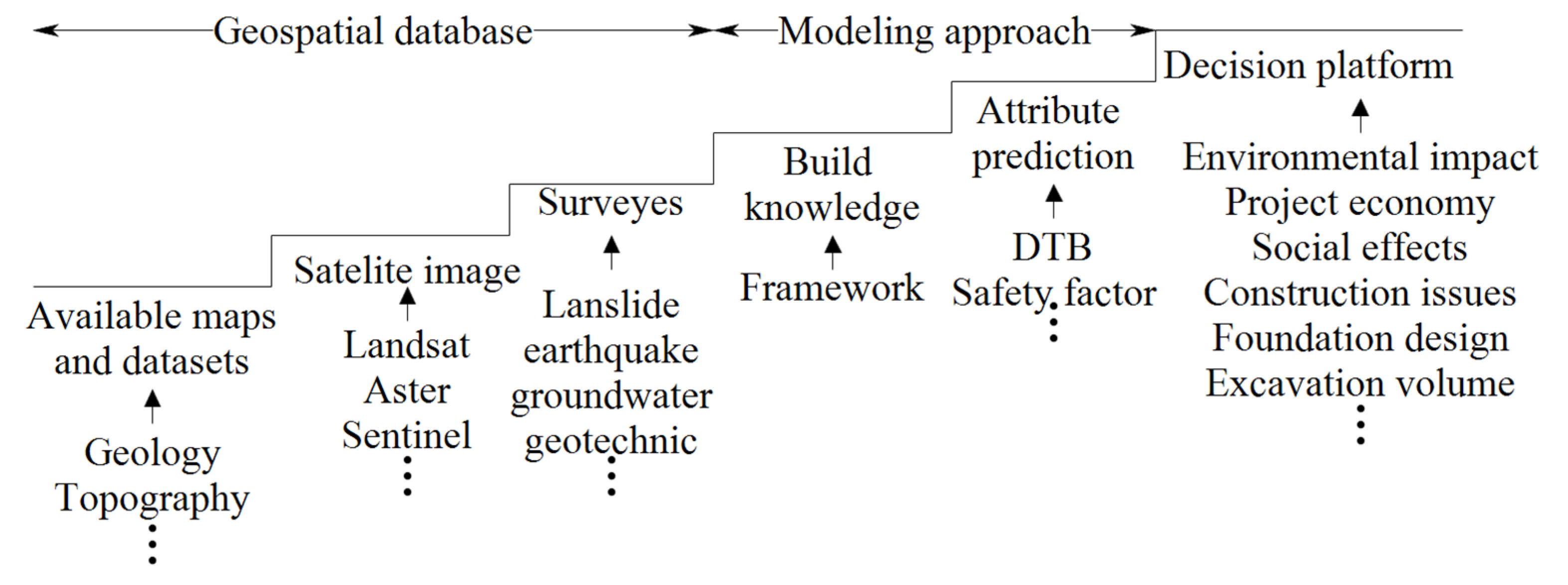
Figure 1 shows the typical steps in providing appropriate geospatial database to dedicate a knowledge-based predictive model. Such a geospatial database involves a wide variety of geo-information, remotely sensed products/images, and site surveys. Depending on the required attribute, the geospatial database can cover DEM, land use, soil type distribution, topographical indices, surface geo-data, drainage pattern of the catchment area, and slope stability, as well as probable natural hazard risks. Accordingly, these incorporations allocate significant economic, social, and environmental benefits for future urbanization and industrial developments on both local and regional scales [27].
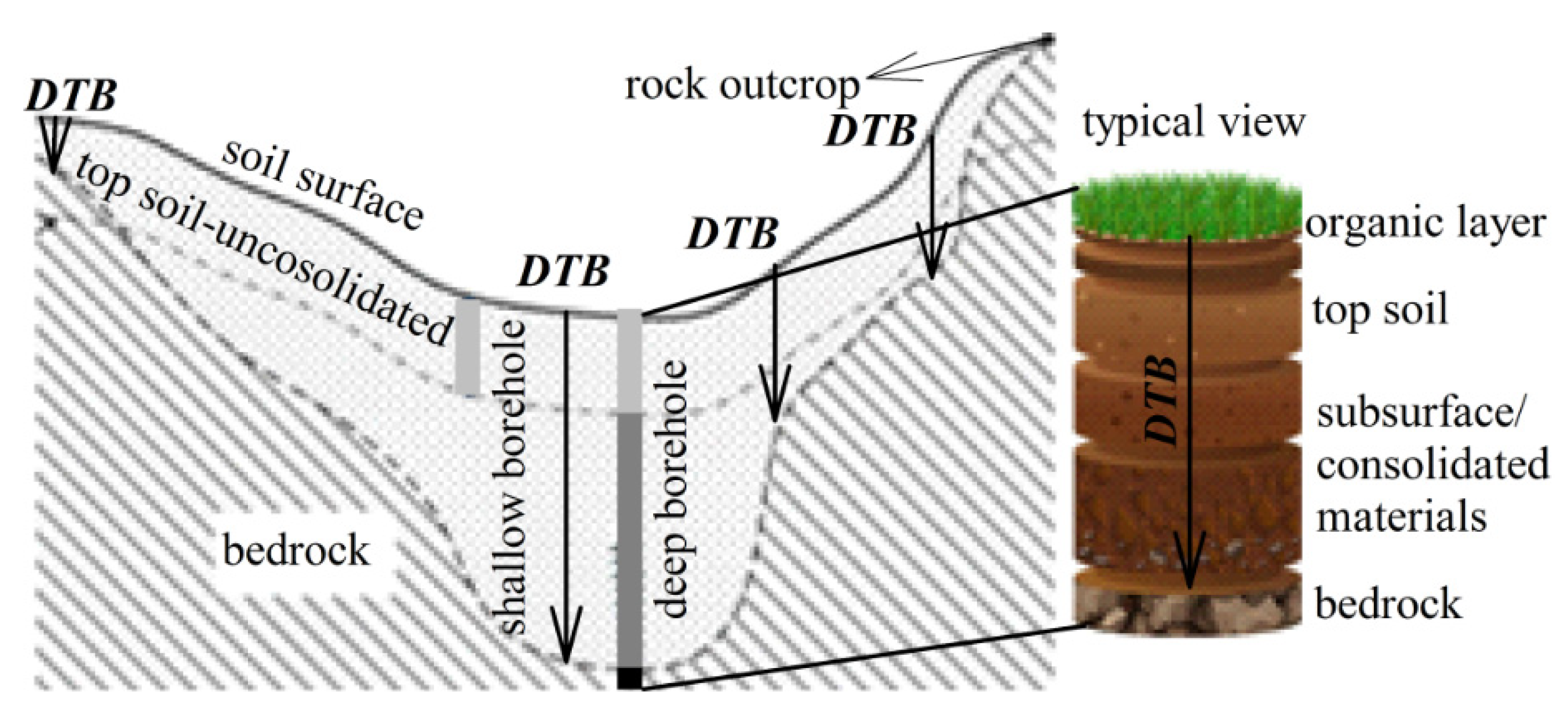
Depth to bedrock (DTB) is one of the interesting subsurface attributes in planning and construction of dams due to significant influence on stability performance and land surface processes [22,23,26]. This attribute (Figure 2) provides knowledge on spatial variation and topographical interface between unconsolidated sediments and stiff layer, as well as more environmental insights to the migration of contaminants following the bedrock gradient [29,30,31]. From an economical perspective, the DTB can significantly impact initialized project costs based on damage, rippability, and excavation volume as well as unnecessary mitigation measures. In foundation design, shallow bedrock requires less overlaid removal for shoring, while deeper distributions can be a liability for lateral variations in soil characteristics [32] and consequently footing and slab failures if not accommodated.
Referring to literatures, the risk of dam project can be reduced through efficient but accurate 3D subsurface spatial DTB model [33,34,35]. However, creating accurate continues predictive spatial DTB model due to densities of sparse surveyed points and imprecise physical data from the material formations as well as associated uncertainties [17,18,36] is usually beyond the ability of traditional applied methods. Furthermore, the observed conflicts of the outcome in predicted DTB subjected to each individual interpolation algorithm [17] evidently describes why it is not always clear which method can provide the most appropriate model.
Gene expression programming (GEP) is an evolutionary computational algorithm for optimization problems, closely related to genetic algorithms and genetic programming [37]. Despite the achieved success of intelligence computational techniques in solving the demerits of DTB models [17,38,39], no distinguished work using GEP for the purpose of subsurface DTB modeling has been reported. Moreover, variability of DTB due to great influence on the stability of dam in high seismic zone such as northern Iran is preferred to be estimated as accurately as possible [40,41,42,43]. This gap motives dedicating an appropriate alternative with supreme predictability levels by introducing a predictive 3D spatial DTB using the GEP. Further, this was applied on a dam site in Guilan province-northern Iran, where high accurate quantitative model is great of interest.
In the current study, the geospatial database was provided using the first three steps presented in Figure 1 through the retrieved information of 63 compiled boreholes, DEM, geology map, and spatial geographical coordinates. The structure of optimum GEP model was captured through programming in C++ with ability in checking wide variety of internal characteristics. It then was compared with conventional ordinary kriging (OK) technique and evaluated using different performance metrics and uncertainty analyses. Then, 82.53% accuracy was observed with R2 = 0.97 in GEP comparing to R2 = 0.92, and 74.6% for OK revealed superior performance in predictions of DTB. These predictions can assist in possible reduction in number of boreholes and corresponding costs.
2. Principle of GEP
The GEP [37] like genetic programming (GP) [44] is an evolutionary intelligent paradigm that originated from genetic algorithms (GAs) [45]. The main fundamental differences between GAs, GP, and GEP are raised due to employed individuals, where the GAs uses linear strings with fixed length (chromosomes) and GP works with nonlinear entities of different sizes and shapes (parse trees). This characteristic in GEP is turned into encoded linear strings of fixed length (the genome or chromosomes) to express nonlinear entities of different sizes and shapes, i.e., simple diagram representations or expression trees (ET).
Referring to Figure 3, the GEP is started with initialized random generated populations (chromosomes) and aims to select and reproduce the individuals using genetic operators and calculated fitness function (FT). The appropriate solution then is found through an iterative procedure comprising three main genetic operators including mutation, transposition, and recombination. If the termination criterion (number of generation) is not achieved, then the process will reproduce new genes using a roulette wheel [46]. Thereby, in the iteration process each chromosome might be modified by none/one or several operators that randomly selects the individuals. In the modification process, the mutation operator essentially is much more effective than others because it can occur in any level of the chromosome. The appropriate value for this operator can be selected within [0.01–0.1] interval [37,46]. Transposition operator internally replaces some consecutive elements of the chromosome. It can be performed using gene, insertion sequence (IS), or root IS (RIS) procedures. The IS provides a copy of randomly selected segment of consecutive elements in tail while in the RIS it is replaced in the heads (roots) of genes. Gene transposition aims to replace the chosen segment of each gene except the first one in the beginning of the chromosome. For transposition, choosing a value in the domain of [0.01–0.1] is recommended [46]. Subsequently, the information of two parent chromosomes using recombination procedure is exchanged to generate two offspring. Therefore, new populations with the same size of the parent but in the form of different sub-ETs are generated that further should be evaluated using the FT.
Each gene of the evolved entities is a fixed length string of different alphabets comprising the head (function and terminal) and tail (terminal). Considering the head (h) as a used defined parameter, the length of the tail (t) is determined by trial error procedure as:
where; n denotes the number of arguments of functions.
Therefore, root of ET (position 0) always is filled by functional operator and subsequently appropriate functions depending on the nature of the problem are attached as branches. The inputs of model are presented in terminals in the form of inclusive variables and numerical constants. Proper functions for the root can be selected among the standard mathematics factors (e.g., +, −, *, /, sqrt, exp, log, ln, sin, cos, etc.) and logical operators (e.g., and, or, not, nor, etc.), as well as Boolean or user defined relations. The corresponding ET then is translated using Kavra language [37] as shown in Figure 4.
3. Study Area and Geospatial Database
Guilan Province lies along the Caspian Sea in the north of Iran which can be characterized using nature and humid subtropical climate with high precipitations. Moreover, part of this territory is in mountainous active Alborlz seismotectonic province that endurea several destructive earthquakes, such as Manji-Roudbar 1990 (Ms7.3). As presented in Figure 5, the Bijar CFRD is suited between the cities of Roudbar and Rasht in Guilan province with 105 Mm3 nominal reservoir capacity, 430 × 10 m crest dimensions and 59.4 m height from the basement.
To provide the geo-database, the 10 × 10 m resolution DEM for the study area (Figure 5) and the corresponding slope were created. The geological and rain fall information from geological survey and meteorological organization of Iran were added to database. The level of overlaid sediments, depth, and geographical coordinates of 63 sparse drilled boreholes and knowledge-based pseudo-observations also were processed and stored in database. These documented geospatial data were then applied to provide DTB predictive topographical model. Referring to Figure 5, the elevation of the area varies between 130 to more than 430 m.
4. DTB Modelling Using GEP
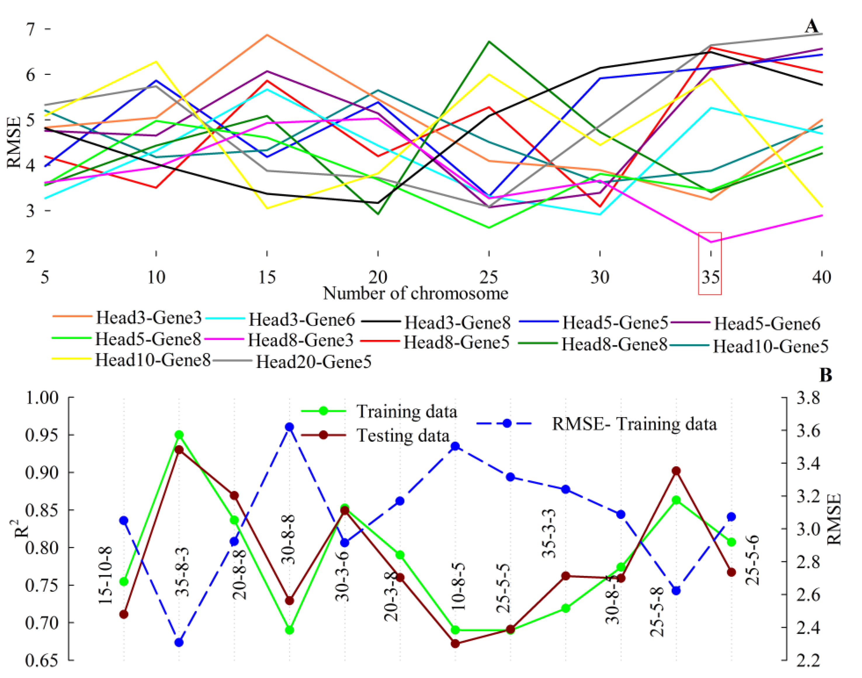
Like all intelligence algorithms, the acquired data should be randomized where the assigned percentage is user defined. Randomizing controls the lurking variable and eliminates the possible biases that may arise in the experiment. In this paper, the values 65%, 20%, and 15% have been considered to build the training, testing, and validation sets. To increase the accuracy of modeling process and get more insights on the area with the lack of data, the expert intelligent knowledge-based approach presented in [17] was applied. The most appropriate number of chromosomes and genes for predictive GEP model was captured subjected to root mean square error (RMSE) as the FT through combination of trial-error and constructive technique [32,47]. Accordingly, the variation of RMSE against the achieved R2 leads to an optimum number of chromosomes, where the predictive GEP structure was selected as the outcome of systemic feedback loops through the changing of internal characteristics. Each individual generated model was checked and controlled to be responsive in serving the required needs. The explained procedure was programmed in C++. Table 1 reflects the ranges of applied parameters in model adjustment.
Figure 6 shows a sample of executed models and corresponding compared performances as a function of numbers of chromosomes and head size. Such parametric investigations revealed that topology of 35-8-3 expressing the number of chromosomes; head size and genes and thus assigned ETs (Figure 7) can be selected as optimal. Accordingly, the ETs of the GEP model then dedicate the mathematical relation as:
5. Comparison, Validation, and Discussion
In the subsurface mapping process of infrastructures, analyses of thematic and surveyed geospatial data due to complexity in both design and construction phases play a fundamental role. Such modeling is a complex task for GIS technology. However, the spatial nature of geo-objects always drives GIS to be part of the modeling systems.
The Dam projects due to vulnerabilities and more susceptibilities require as accurate as possible information on subsurface conditions. Accordingly, unavailability of accurate enough subsurface maps can create a challenging situation and intensify facing the un-considered and unexpected problems in the planning and construction process. Moreover, autocorrelation, heterogeneity, limited ground truth, and multiple scales and resolutions also poses unique challenges [48] that violate common employed assumption of many traditional predictive modeling [49]. As most exploratory boreholes are randomly distributed and may not be representative over the study area, selecting the best interpolation method giving the closest approximation to known parameters is usually difficult but imperative [50]. Therefore, predictive spatial models are developed to increase the resolution of the response variable based on explanatory features. Since the systematic surveys of underground are critical, mapping and modeling of subsurface helps to mitigate the risk from a utility-congested scenario. Combining innovative technologies such as BIM was also found to be critical in reducing the engineering risks associated with the subsurface construction site [10,11].
From an engineering perspective, generated models need to be pursued for validation and check for the compliance and system realization. Such a process aims to ensure that the produced model meets the accuracy and operational criteria. In this paper, comparing the results with OK geostatistical technique, accuracy performance using confusion matrix and statistical error criteria, as well as uncertainty analyses through confidence and prediction intervals (CI and PI), were carried out.
Kriging [51] is a recognized applicable geostatistical interpolation technique for the unknown values of spatial and temporal variables. Governing by prior covariances through the Gaussian process regression, this algorithm dedicates the best practical unbiased prediction for intermediate values [52]. Among the different types of kriging, the OK can implicitly evaluate the mean in a moving neighborhood as well as estimating a block value [53]. This method presents a minimized estimation of variance through the optimal weights to reduce the error [45] as:
where; γ is the variogram value. zi and Xi denote the real and estimated values at location i, respectively. λi shows the assigned weighting coefficient and μ is Lagrange factor.
The performance and comparison between the OK and GEP model subjected to randomized datasets are shown in Figure 10A. The level of CI represents a visual sense for long-term success of the method in capturing the DTB, while PI shows the certain probability of future estimation. The stability and capacity of GEP and OK predictive models using employed data was reflected in Figure 10B. Statistically, the predictive model is in control if the outputs fall within certain ranges where the wider CI, the more instable the relation. Residual as the difference between the observed and predicted indicates the fitting deviation and is presented in Figure 10C.
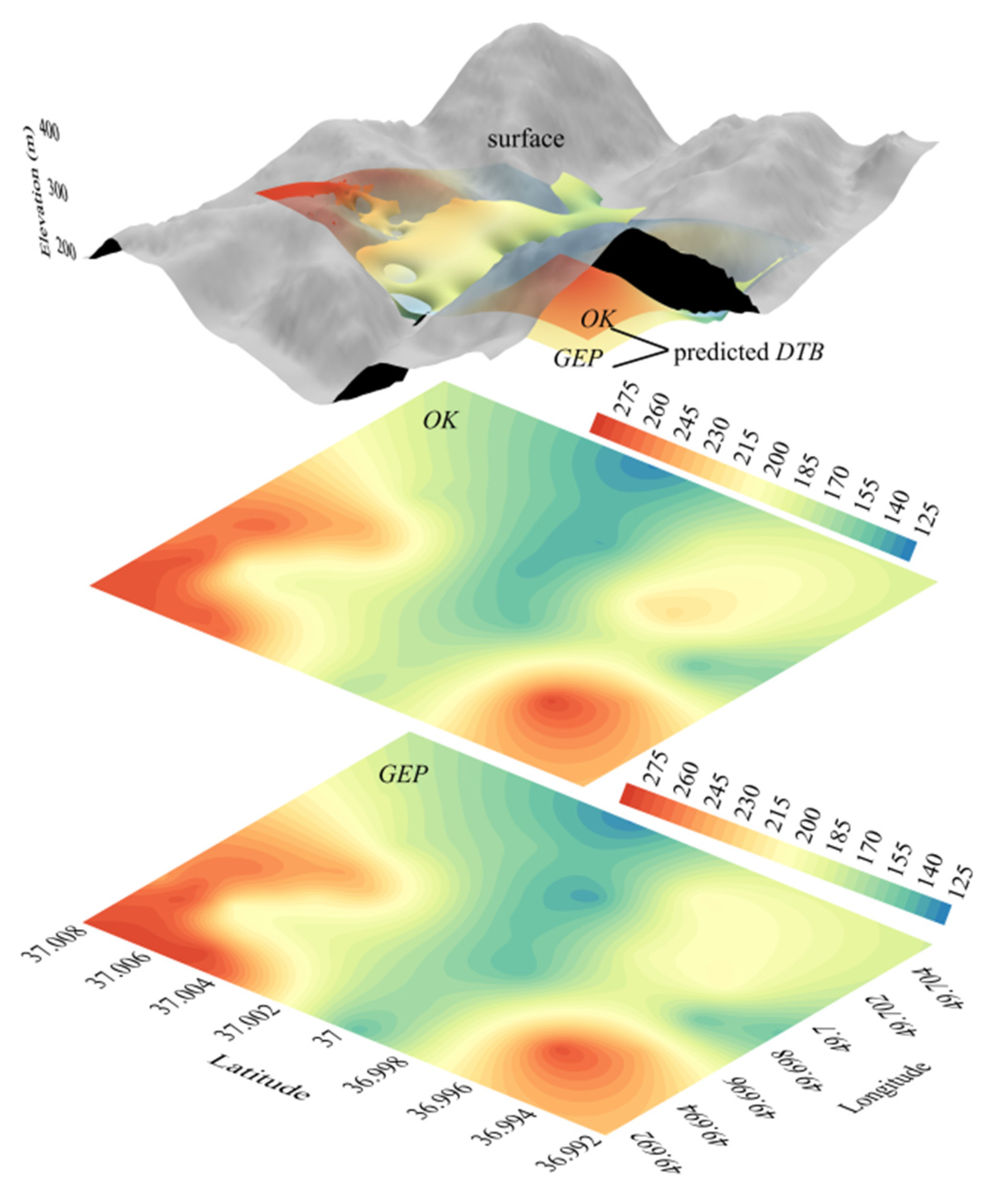
Visual comparison describing the predictability level of OK and GEP using confusion matrix [54] is given in Table 2, where each array dedicates the number of true labeled outputs. The results showed 82.53% performance in accurate data labeling in GEP and 9.61% improvement than the OK. The perspectives of 3D generated models then are presented in Figure 11.
The performance of predictive model including quantitative numerical values can be scaled and compared using statistical error metrics such as mean absolute percentage error (MAPE), RMSE, R2, and residuals. The MAPE is one of the most popular indexes for description of accuracy and size of the forecasting error, while residual represents a fitting deviation of predicted value from measured. RMSE expresses the prediction accuracy of a model and is an appropriate estimator for the standard deviation of the error distribution. R2 reflect the goodness of fit in prediction problem. As presented in Figure 12, higher values of R2 as well as smaller MAPE, residual, and RMSE are interpreted as more accurate levels (Figure 11).
6. Concluding Remarks
Developing accurate enough subsurface topographical predictive models can address new challenges in both infrastructure and urbanized scales. On a regional scale, 3D models can completely tie geospatial databases into subsurface models. Accordingly, unforeseen subsurface conditions due to incomplete information can cause large incurred indirect costs. This leads to a higher quality database, superior knowledge, and thus more visualized insights on new opportunities. It then leads to more tailored planning and management of increased subsurface uses and thus wider and long-term benefits.
These concerns stimulated checking performance of GEP evolutionary algorithms in subsurface analyses where high-resolution and more accurate predictive DTB models significantly are demanded. The capabilities of programmed GEP in C++ then was pursued in Bijar CFRD dam, north of Iran, and compared with OK. According to obtained results, the GEP model showed 9.81% progress more than OK in predictability levels of DTB. Analyzed control performance in terms of MAPE, RMSE, residual, and R2 reflected supreme performance in GEP than OK. Referring to established CI and PI more stability in model and thus future prediction in GEP rather than the OK is expected. The compared results revealed that OK provides over/underestimate more results than GEP and thus can generate unrepresentative interpolation for the entire of the studied area. This implies that GEP efficiently dedicates more cost-effective and accurate enough prediction for the DTB.
From a practical perspective, DTB mapping can assist in distinguishing infill sediments. It can be applied for modeling the landscape evolution, natural hazard assessments, and groundwater evaluation to help decision makers in assessing the risk patterns and promote new responses to detect out of the ordinary behavior before serious damages are inflicted.
Author Contributions
Conceptualization, Abbas Abbaszadeh Shahri and Ali Kheri; software, Aliakbar Hamzeh and Abbas Abbaszadeh Shahri; validation, Abbas Abbaszadeh Shahri, Ali Kheri and Aliakbar Hamzeh; formal analysis, Abbas Abbaszadeh Shahri, Ali Kheiri and Aliakbar Hamzeh; Data curation, Abbas Abbaszadeh Shahri and Ali Kheiri; writing—original draft preparation, Abbas Abbaszadeh Shahri; writing—review and editing, Abbas Abbaszadeh Shahri, Ali Kheri and Aliakbar Hamzeh. All authors have read and agreed to the published version of the manuscript.
Funding
This research received no external funding.
Institutional Review Board Statement
Not applicable.
Informed Consent Statement
Not applicable.
Data Availability Statement
The information on DEM, geological setting and rain fall data publicly can be found in https://earthexplorer.usgs.gov (accessed on 16 May 2021); www.gsi.ir (accessed on 16 May 2021) and www.irimo.ir (accessed on 16 May 2021).
Conflicts of Interest
The authors declare no conflict of interest.
References
- Kotsev, A.; Minghini, M.; Tomas, R.; Cetl, V.; Lutz, M. From Spatial Data Infrastructures to Data Spaces- A Technological Perspective on the Evolution of European SDIs. ISPRS Int. J. Geo Inf. 2020, 9, 176. [Google Scholar] [CrossRef] [Green Version]
- Li, D.; Wang, S.; Yuan, H.; Li, D. Software and Applications of Spatial Data Mining. Wiley Interdiscip. Rev. Data Min. Knowl. Discov. 2016, 6, 84–114. [Google Scholar] [CrossRef]
- Ristoski, P.; Paulheim, H. Semantic Web in Data Mining and Knowledge Discovery: A Comprehensive Survey. J. Web Semant. 2016, 36, 1–22. [Google Scholar] [CrossRef] [Green Version]
- Gervone, G.; Lin, J.; Waters, N. Data Mining for Geoinformatics: Methods and Applications; Springer: New York, NY, USA, 2014. [Google Scholar]
- Omidipoor, M.; Toomanian, A.; Samany, N.N.; Mansourian, A. Knowledge Discovery Web Service for Spatial Data Infrastructures. ISPRS Int. J. Geo Inf. 2021, 10, 12. [Google Scholar] [CrossRef]
- Sikder, S.K.; Behnisch, M.; Herold, H.; Koetter, T. Geospatial Analysis of Building Structures in Megacity Dhaka: The Use of Spatial Statistics for Promoting Data-driven Decision-making. J. Geovis. Spat. Anal. 2019, 3, 7. [Google Scholar] [CrossRef]
- Reichstein, M.; Camps-Valls, G.; Stevens, B.; Jung, M.; Denzler, J.; Carvalhais, N. Prabhat. Deep Learning and Process Understanding for Data-driven Earth System Science. Nature 2019, 566, 195–204. [Google Scholar] [CrossRef]
- Darabi, H.; Haghighi, A.T.; Mohamadi, M.A.; Rashidpour, M.; Ziegler, A.D.; Hekmatzadeh, A.A.; Kløve, B. Urban Flood Risk Mapping Using Data-driven Geospatial Techniques for a Flood-prone Case Area in Iran. Hydrol. Res. 2020, 51, 127–142. [Google Scholar] [CrossRef] [Green Version]
- Senanayake, S.; Pradhan, B.; Huete, A.; Brennan, J. A Review on Assessing and Mapping Soil Erosion Hazard Using Geo-informatics Technology for Farming System Management. Remote Sens. 2020, 12, 4063. [Google Scholar] [CrossRef]
- Ma, Z.; Ren, Y. Integrated Application of BIM and GIS: An Overview. Procedia Eng. 2017, 96, 1072–1079. [Google Scholar] [CrossRef]
- Song, Y.; Wang, X.; Tan, Y.; Wu, P.; Sutrisna, M.; Cheng, J.C.P.; Hampson, K. Trends and Opportunities of BIM-GIS Integration in the Architecture, Engineering and Construction Industry: A Review from a Spatio-temporal Statistical Perspective. ISPRS Int. J. Geo Inf. 2017, 6, 397. [Google Scholar] [CrossRef] [Green Version]
- Abbaszadeh Shahri, A.; Spross, J.; Johansson, F.; Larsson, S. Landslide Susceptibility Hazard Map in Southwest Sweden Using an Artificial Neural Network. Catena 2019, 183, 104225. [Google Scholar] [CrossRef]
- De Roo, A.P.J. Soil Erosion Assessment Using G.I.S. In Geographical Information Systems in Hydrology; Singh, V.P., Fiorentino, M., Eds.; Springer: Dordrecht, The Netherlands, 1996; pp. 339–356. [Google Scholar]
- Zhou, K.; Xie, Y.; Gao, Z.; Miao, F.; Zhang, L. FuNet: A Novel Road Extraction Network with Fusion of Location Data and Remote Sensing Imagery. ISPRS Int. J. Geo Inf. 2021, 10, 39. [Google Scholar] [CrossRef]
- Bai, J.; Zhou, Z.; Zou, Y.; Pulatov, B.; Siddique, K.H.M. Watershed Drought and Ecosystem Services: Spatiotemporal Characteristics and Gray Relational Analysis. ISPRS Int. J. Geo Inf. 2021, 10, 43. [Google Scholar] [CrossRef]
- Abbaszadeh Shahri, A.; Maghsoudi Moud, F. Landslide Susceptibility Mapping Using Hybridized Block Modular Intelligence Model. Bull. Eng. Geol. Environ. 2021, 80, 267–284. [Google Scholar] [CrossRef]
- Abbaszadeh Shahri, A.; Larsson, S.; Renkel, C. Artificial Intelligence Models to Generate Visualized Bedrock Level: A Case Study in Sweden. Model. Earth Syst. Environ. 2020, 6, 1509–1528. [Google Scholar] [CrossRef]
- Nath, R.R.; Kumar, G.; Sharma, M.L.; Gupta, S.C. Estimation of Bedrock Depth for a Part of Garhwal Himalayas Using Two Different Geophysical Techniques. Geosci. Lett. 2018, 5, 9. [Google Scholar] [CrossRef] [Green Version]
- Li, Z.; Li, W.; Ge, W. Weight Analysis of Influencing Factors of Dam Break Risk Consequences. Nat. Hazards Earth Syst. Sci. 2018, 18, 3355–3362. [Google Scholar] [CrossRef] [Green Version]
- Ge, W.; Li, Z.; Liang, R.Y.; Li, W.; Cai, Y. Methodology for Establishing Risk Criteria for Dams in Developing Countries, Case Study of China. Water Resour. Manag. 2017, 31, 4063–4074. [Google Scholar] [CrossRef]
- Jozaghi, A.; Alizadeh, B.; Hatami, M.; Flood, I.; Khorrami, M.; Khodaei, N.; Ghasemi Tousi, E. A Comparative Study of the AHP and TOPSIS Techniques for Dam Site Selection Using GIS: A Case Study of Sistan and Baluchestan Province, Iran. Geosciences 2018, 8, 494. [Google Scholar] [CrossRef] [Green Version]
- Pourghasemi, H.R.; Yusefi, S.; Nitheshnirmal, S.; Eskandari, S. Assessing, Mapping, and Optimizing the Locations of Sediment Control Check Dams Construction. Sci. Total Environ. 2020, 739, 139954. [Google Scholar] [CrossRef]
- Al-Ruzouq, R.; Shanableh, A.; Yilmaz, A.G.; Idris, A.; Mukherjee, S.; Khalil, M.A.; Gibril, M.B.A. Dam Site Suitability Mapping and Analysis Using an Integrated GIS and Machine Learning Approach. Water 2019, 11, 1880. [Google Scholar] [CrossRef] [Green Version]
- Kim, H.S.; Chung, C.K.; Kim, H.K. Geo-spatial Data Integration for Subsurface Stratification of Dam Site with Outlier Analyses. Environ. Earth Sci. 2016, 75, 168. [Google Scholar] [CrossRef]
- Sissakian, V.K.; Adamo, N.; Al-Ansari, N. The Role of Geological Investigations for Dam Siting: Mosul Dam a Case Study. Geotech. Geol. Eng. 2020, 38, 2085–2096. [Google Scholar] [CrossRef] [Green Version]
- Malczewski, J. GIS-based Land-use Suitability Analysis: A Critical Overview. Prog. Plan. 2004, 62, 3–65. [Google Scholar] [CrossRef]
- Li, S.; Dragicevic, S.; Castroc, F.A.; Sester, M.; Winter, S.; Coltekin, A.; Pettitg, C.; Jiang, B.; Haworth, J.; Stein, A.; et al. Geospatial Big Data Handling Theory and Methods: A Review and Research Challenges. ISPRS J. Photogramm. Remote Sens. 2016, 115, 119–133. [Google Scholar] [CrossRef] [Green Version]
- Turner, A.K. Geoscientific Modeling: Past, Present, and Future. In AAPG Computer Application in Geology, No. 4: Geographic Information Systems in Petroleum Exploration and Development; Coburn, T.C., Yarus, J.M., Eds.; The American Association of Petroleum Geologists: Tulsa, OK, USA, 2000; pp. 27–36. [Google Scholar]
- Zhang, C.; Chai, J.; Cao, J.; Xu, Z.; Qin, Y.; Lv, Z. Numerical Simulation of Seepage and Stability of Tailings Dams: A Case Study in Lixi, China. Water 2020, 12, 742. [Google Scholar] [CrossRef] [Green Version]
- Jardine, P.M.; Sanford, W.E.; Gwo, J.P.; Reedy, C.; Hicks, D.S.; Riggs, J.S.; Bailey, W.B. Quantifying Diffusive Mass Transfer in Fractured Shale Bedrock. Water Resour. Res. 1999, 35, 2015–2030. [Google Scholar] [CrossRef]
- Bondu, R.; Cloutier, V.; Rosa, E. Occurrence of Geogenic Contaminants in Private Wells from a Crystalline Bedrock Aquifer in Western Quebec, Canada: Geochemical Sources and Health Risks. J. Hydrol. 2018, 559, 627–637. [Google Scholar] [CrossRef]
- Ghaderi, A.; Abbaszadeh Shahri, A.; Larsson, S. An Artificial Neural Network Based Model to Predict Spatial Soil Type Distribution Using Piezocone Penetration Test Data (CPTu). Bull. Eng. Geol. Environ. 2019, 78, 4579–4588. [Google Scholar] [CrossRef] [Green Version]
- Salih, S.A.; Al-Tarif, A.M. Using of GIS Spatial Analyses to Study the Selected Location for Dam Reservoir on Wadi Al-Jirnaf, West of Shirqat Area, Iraq. J. Geogr. Inf. Syst. 2012, 4, 117–127. [Google Scholar] [CrossRef] [Green Version]
- Kavoura, K.; Konstantopoulou, M.; Kyriou, A.; Nikolakopoulos, K.G.; Sabatakakis, N.; Depountis, N. 3D Subsurface Geological Modeling Using GIS, Remote Sensing, and Boreholes Data. In Proceedings of the Fourth International Conference on Remote Sensing and Geoinformation of the Environment, Paphos, Cyprus, 4–8 April 2016. [Google Scholar] [CrossRef]
- Balasubramani, D.P.; Dodagoudar, G.R. An Integrated Geotechnical Database and GIS for 3D Subsurface Modelling: Application to Chennai City, India. Appl. Geomat. 2018, 10, 47–64. [Google Scholar] [CrossRef]
- Yan, F.; Shangguan, W.; Zhang, J.; Hu, B. Depth-to-bedrock Map of China at a Spatial Resolution of 100 Meters. Sci. Data 2020, 7, 2. [Google Scholar] [CrossRef] [PubMed] [Green Version]
- Ferreira, C. Gene Expression Programming: A New Adaptive Algorithm for Solving Problems. Complex Syst. 2001, 13, 87–129. [Google Scholar]
- Samui, P.; Kumari, S.; Makarov, V.; Kurup, P. Modeling in Geotechnical Engineering; Elsevier: Cambridge, MA, USA, 2020. [Google Scholar]
- Chang, J.R.; Chao, S.J. Applying Group Method of Data Handling (GMDH) Method to Predict Depth to Bedrock. Comput. Civ. Eng. 2009. [Google Scholar] [CrossRef]
- Tempa, K.; Sarkar, R.; Dikshit, A.; Pradhan, B.; Simonelli, A.L.; Acharya, S.; Alamri, A.M. Parametric Study of Local Site Response for Bedrock Ground Motion to Earthquake in Phuentsholing, Bhutan. Sustainability 2020, 12, 5273. [Google Scholar] [CrossRef]
- Manandhar, S.; Cho, H.I.; Kim, D.S. Effect of Bedrock Stiffness and Thickness of Weathered Rock on Response Spectrum in Korea. KSCE J. Civ. Eng. 2016, 20, 2677–2691. [Google Scholar] [CrossRef]
- Gomes, G.J.C.; Vrugt, J.A.; Vargas, E.A., Jr.; Camargo, J.T.; Velloso, R.Q.; van Genuchten, M.T. The Role of Uncertainty in Bedrock Depth and Hydraulic Properties on the Stability of a Variably-saturated Slope. Comput. Geotech. 2017, 88, 222–241. [Google Scholar] [CrossRef] [Green Version]
- Boore, D.M. Estimating Vs(30) (or NEHRP Site Classes) from Shallow Velocity Models (Depths < 30 m). Bull. Seismol. Soc. Am. 2004, 94, 591–597. [Google Scholar] [CrossRef]
- Koza, J.R. Genetic Programming: On the Programming of Computers by Means of Natural Selection; MIT Press: Camridge, MA, USA, 1992. [Google Scholar]
- Goldberg, D.E.; Holland, J.H. Genetic Algorithms and Machine Learning. Mach. Learn. 1988, 3, 95–99. [Google Scholar] [CrossRef]
- Ferreira, C. Gene Expression Programming: Mathematical Modeling by an Artificial Intelligence, 2nd ed.; Springer: Berlin, Germany, 2006. [Google Scholar]
- Asheghi, R.; Abbaszadeh Shahri, A.; Khorsand Zak, M. Prediction of Strength Index Parameters of Different Rock Types Using Hybrid Multi Output Intelligence Model. Arab. J. Sci. Eng. 2019, 44, 8645–8659. [Google Scholar] [CrossRef]
- Jiang, Z. A Survey on Spatial Prediction Methods. IEEE Trans. Knowl. Data Eng. 2019, 31, 1645–1664. [Google Scholar] [CrossRef]
- Frank, R.; Ester, M.; Knobbe, A. A Multi-rational Approach to Spatial Classification. In Proceedings of the KDD09: The 15th ACM SIGKDD International Conference on Knowledge Discovery and Data Mining, Paris, France, 28 June–1 July 2009; pp. 309–318. [Google Scholar] [CrossRef] [Green Version]
- Bamisaiye, O.A. Subsurface Mapping: Selection of Best Interpolation Method for Borehole Data Analysis. Spat. Inf. Res. 2018, 26, 261–269. [Google Scholar] [CrossRef]
- Krige, D.G. A Statistical Approach to some Basic Mine Valuation Problems on the Witwatersrand. J. Chem. Metal. Mining Soc. S. Afr. 1951, 52, 119–139. [Google Scholar]
- Wackernagel, H. Ordinary Kriging. In Multivariate Geostatistics; Springer: Berlin/Heidelberg, Germany, 1999; pp. 74–81. [Google Scholar]
- Saveliev, A.A.; Mukharamova, S.S.; Chizhikova, N.A.; Budgey, R.; Zuur, A.F. Spatially Continuous Data Analysis and Modelling. In Analysing Ecological Data. Statistics for Biology and Health; Springer: New York, NY, USA, 2007. [Google Scholar]
- Stehman, S.V. Selecting and Interpreting Measures of Thematic Classification Accuracy. Remote Sens. Environ. 1999, 62, 77–89. [Google Scholar] [CrossRef]
Figure 1.
Toward decision platform using geospatial database.

Figure 2.
Applied terminology in DTB definition.

Figure 3.
Flow diagram of GEP algorithm.

Figure 4.
ETs expression and coded chromosome for (A) three and (B) two genes denoting the head (H) and tail (T). The vertical arrow corresponding to bolded characters show the termination point of each gene (A).
Figure 4.
ETs expression and coded chromosome for (A) three and (B) two genes denoting the head (H) and tail (T). The vertical arrow corresponding to bolded characters show the termination point of each gene (A).

Figure 5.
Location of studied area in Iran (A) and Guilan province (B), generated DEM and overlaid spatial data (C), and distribution of geospatial surveyed drilled boreholes (D).
Figure 5.
Location of studied area in Iran (A) and Guilan province (B), generated DEM and overlaid spatial data (C), and distribution of geospatial surveyed drilled boreholes (D).

Figure 6.
(A) Variation of RMSE for series parametric analyses using different head size and genes based on the number of chromosomes, (B) evaluated candidate models using RMSE and R2.
Figure 6.
(A) Variation of RMSE for series parametric analyses using different head size and genes based on the number of chromosomes, (B) evaluated candidate models using RMSE and R2.

Figure 7.
The ETs expression of selected optimum GEP model.

Figure 8.
Predictability of developed GEP model using employed datasets.

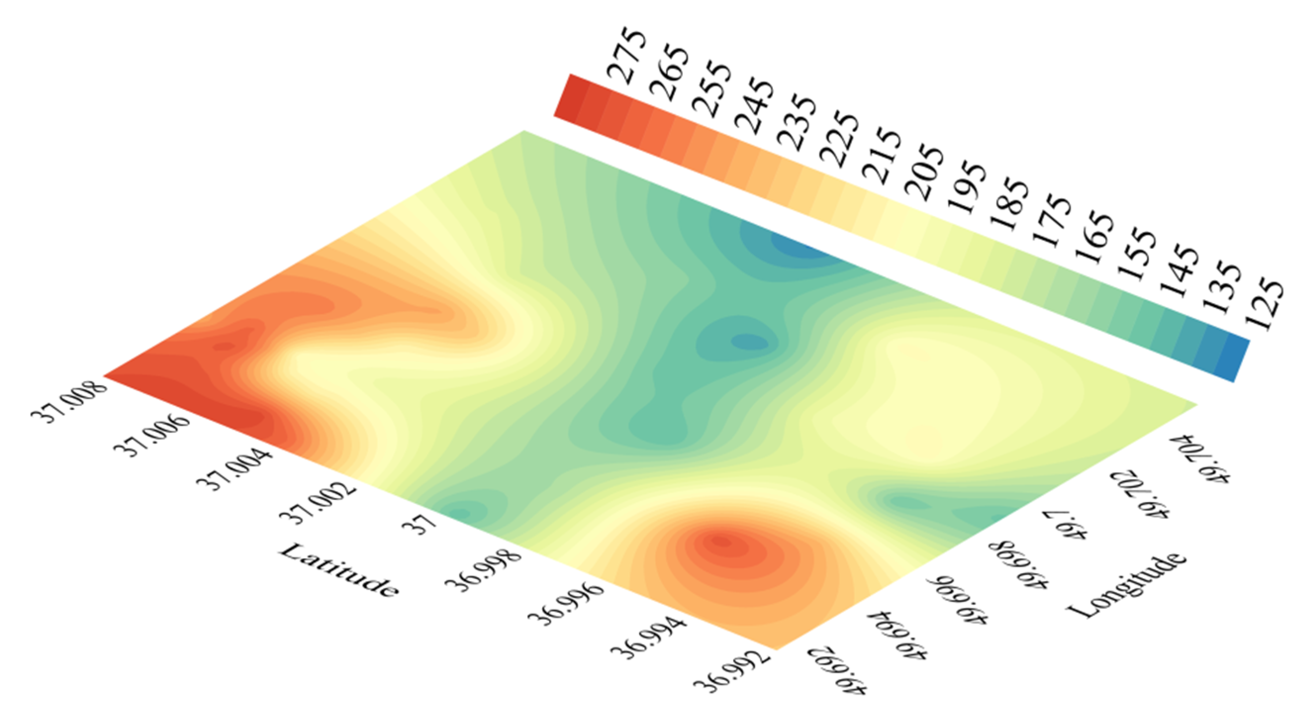
Figure 9.
Predicted spatial DTB using optimum GEP topology.

Figure 10.
Results of OK (A), predictability of OK and GEP using CI and PI (B) and compared residuals (C).
Figure 10.
Results of OK (A), predictability of OK and GEP using CI and PI (B) and compared residuals (C).

Figure 11.
Visualized insights into predicted spatial DTB models using optimum GEP and OK.

Figure 12.
Compared performance of models using statistical error metrics for whole datasets (delete the dot line).
Figure 12.
Compared performance of models using statistical error metrics for whole datasets (delete the dot line).


Table 1.
The range of applied parameters in adjusting GEP model.
| Parameter | Value | Parameter | Value |
|---|---|---|---|
| chromosome | [5,40] | link function | + |
| head size | [3,20] | mutation rate | 0.02, 0.04 |
| number of genes | 3, 5, 6, 8, 10 | inversion | 0.1, 0.3 |
| generation | [500,2000] | population size | [1,100] |
| IS | 0.1, 0.3 | RIS | 0.1, 0.3 |
| recombination rate | 0.3 | gene recombination rate | 0.1 |
| gene transposition rate | 0.1 | one/two-point recombination rate | 0.027 |
| used function | +, −, *, /, sqrt(x), exp(x), pow10, log(x), 1/x, −x, x2, x3, x1/3, sin(x), cos(x), actan(x),1−x | ||
Table 2.
Predictability and observed improvement of GEP and OK (The bolded numbers are referred to GEP).
Table 2.
Predictability and observed improvement of GEP and OK (The bolded numbers are referred to GEP).
| Predicted Output | Results | ||||||||||||||
|---|---|---|---|---|---|---|---|---|---|---|---|---|---|---|---|
| Target | [<128.7] | [128.7–143.57] | [143.57–158.44] | [158.44–173.31] | [173.31–188.18] | [188.18–203.05] | [203.05–217.92] | [217.92–232.79] | [232.79–247.66] | [247.66–262.53] | [262.53–277.4] | [>277.4] | Total | True | False |
| <128.7 | 0 | 0,0 | 0,0 | ||||||||||||
| [128.7–143.57] | 0,1 | 1,0 | 1,1 | 2 | 1,0 | 1,2 | |||||||||
| [143.57–158.44] | 1,1 | 6,6 | 1,1 | 8 | 6,6 | 2,2 | |||||||||
| [158.44–173.31] | 1,1 | 1,1 | 2 | 1,1 | 1,1 | ||||||||||
| [173.31–188.18] | 1,0 | 5,5 | 1,0 | 0,1 | 0,1 | 7 | 5,5 | 2,2 | |||||||
| [188.18–203.05] | 8,7 | 1,1 | 0,1 | 9 | 8,7 | 1,2 | |||||||||
| [203.05–217.92] | 0,1 | 9,7 | 0,1 | 9 | 9,7 | 0,2 | |||||||||
| [217.92–232.79] | 2,3 | 1,0 | 3 | 2,3 | 1,0 | ||||||||||
| [232.79–247.66] | 0,1 | 1,0 | 5,4 | 0,1 | 6 | 5,4 | 1,2 | ||||||||
| [247.66–262.53] | 1,0 | 4,4 | 0,1 | 5 | 4,4 | 1,1 | |||||||||
| [262.53–277.4] | 1,2 | 11,10 | 0,1 | 12 | 11,10 | 1,2 | |||||||||
| [>277.4] | 0 | 0,0 | 0,0 | ||||||||||||
| Bold values: GEP | 52,47 | 11,16 | |||||||||||||
| Accurate labeled data (%) 82.53%,74.6% | |||||||||||||||
Publisher’s Note: MDPI stays neutral with regard to jurisdictional claims in published maps and institutional affiliations. |
© 2021 by the authors. Licensee MDPI, Basel, Switzerland. This article is an open access article distributed under the terms and conditions of the Creative Commons Attribution (CC BY) license (https://creativecommons.org/licenses/by/4.0/).
Share and Cite
MDPI and ACS Style
Abbaszadeh Shahri, A.; Kheiri, A.; Hamzeh, A. Subsurface Topographic Modeling Using Geospatial and Data Driven Algorithm. ISPRS Int. J. Geo-Inf. 2021, 10, 341. https://doi.org/10.3390/ijgi10050341
AMA Style
Abbaszadeh Shahri A, Kheiri A, Hamzeh A. Subsurface Topographic Modeling Using Geospatial and Data Driven Algorithm. ISPRS International Journal of Geo-Information. 2021; 10(5):341. https://doi.org/10.3390/ijgi10050341
Chicago/Turabian StyleAbbaszadeh Shahri, Abbas, Ali Kheiri, and Aliakbar Hamzeh. 2021. "Subsurface Topographic Modeling Using Geospatial and Data Driven Algorithm" ISPRS International Journal of Geo-Information 10, no. 5: 341. https://doi.org/10.3390/ijgi10050341
Note that from the first issue of 2016, this journal uses article numbers instead of page numbers. See further details here.