
A Novel Robust Approach for Computing DE-9IM Matrices Based on Space Partition and Integer Coordinates


1
Faculty of Spatial Information, Hochschule für Technik und Wirtschaft Dresden University of Applied Sciences, 01069 Dresden, Germany
2
Faculty VI Planning Building Environment, Institute of Civil Engineering, Technische Universität Berlin, 13353 Berlin, Germany
*
Author to whom correspondence should be addressed.
ISPRS Int. J. Geo-Inf. 2021, 10(11), 715; https://doi.org/10.3390/ijgi10110715
Submission received: 10 August 2021
/
Revised: 14 October 2021
/
Accepted: 15 October 2021
/
Published: 20 October 2021
Abstract
:A novel approach for a robust computation of positional relations of two-dimensional geometric features is presented which guarantees reliable results, provided that the initial data is valid. The method is based on the use of integer coordinates and a method to generate a complete, gap-less and non-overlapping spatial decomposition. The spatial relationships of two geometric features are then represented using DE-9IM matrices. These allow the spatial relationships to be represented compactly. The DE-9IM matrices are based on the spatial decomposition using explicit neighborhood relations. No further geometric calculations are required for their computation. Based on comparative tests, it could be proven that this approach, up to a predictable limit, provides correct results and thus offers advantages over classical methods for the calculation of spatial relationships. This novel method can be used in all fields, especially where guaranteed reliable results are required.
1. Introduction
An important functionality in GIS or CAD is the calculation of spatial relations of geographic or geometric objects (features). There are many publications dealing with the efficient and correct representation of these relations. This article is not about the different types of representations and their advantages and disadvantages, it is about the correct calculation of spatial relations.
On the one hand, a correct calculation of spatial relations is based on exact geometric computations and, on the other hand, on consistent topological relations. Exact geometric computations cannot be guaranteed in every case if floating point numbers are used. Nevertheless, floating point numbers are mostly used for computation (see e.g., Ref. [1]). This problem can be easily solved by using integer numbers. Also, in any case it must be guaranteed that the topology is consistent with the geometry, this is especially a problem when the features to be compared come from different data sources.
We developed an algorithm that overcomes these problems. The method is based on three fundamental principles:
- The use of integer coordinates and the representation of intersections as positions on edges using rational numbers.
- An algorithm for generating a complete, gapless and non-overlapping spatial decomposition.
- The generation of DE-9IM matrices without further geometric calculations by set operations of special types.
The main goal of our algorithm is to guarantee consistency between geometrical and topological relations of 2D features. In the following we will prove that the presented approach can achieve this for geospatial data, when determine topological relations (DE-9IM) or checking geometric features for topological inconsistencies. To illustrate the practical relevance, we will show that conventional geo tools fail to achieve the main goal under certain conditions. In our analysis, we compare our approach with the NetTopologySuite library and the SpatiaLite database. Although this is only a small selection, it should only serve to highlight the basic problem.
As an illustration, point P(A) (a point of feature A) and edge E(3) (an edge of feature 3) are highlighted in Figure 1a. A question about point P(A) would be: is it in feature 1 or 2, or even directly on the edge between the two features? Similarly for edge E(3): does this cross feature B or is it on an edge? Topology and geometry should be consistent for clear resolutions of these questions.
In step one, the vertex coordinates of the original geometries are converted into integer coordinates. This step guarantees that after the conversion the geometric calculations are unambiguous. For this purpose, the coordinates are scaled so that they can be represented as integers without changing their relative position to each other (Figure 1b). In this step it is possible to check the validity of the given features (now represented with integer coordinates), based on their properties such as length, area and orientation.
In the second step, a spatial decomposition consisting of vertices, edges and faces is generated (Figure 1d). As a first sub-step, a triangulation of all points is generated (Figure 1c). This triangulation forms the base mesh and guarantees that the spatial decomposition is gap-less. Then the edges of the features are reconstructed in this base mesh. This special algorithm guarantees that the model represents the correct topological relations of the initial geometries. The generated spatial decomposition is then complete, gap-less and non-overlapping. To achieve this, the edge intersections are represented as ordered positions on the edges using rational numbers. Since their number range is predictable, no data type for arbitrarily large integers is needed.
The generated spatial decomposition contains all geometrical and topological information of the source geometries; thus it is possible to determine the spatial relations without further geometrical calculations. To facilitate the queries, special 0, 1 and 2 dimensional objects are created, each representing a source feature. This is the last instance where incorrect source geometries can be detected and filtered out. Then, the DE-9IM matrices can be generated efficiently without geometric calculations, purely by set operations.
2. Related Research
The problem area of exact results of geometrical calculations is considered in many publications (e.g., Refs. [2,3,4,5]). It is called “exact geometry”, “exact computation”, “geometric predicates” or “exact geometric computation”. An overview of the problem area is provided in [6]. The problem is usually considered from the computational side. One can say that integer coordinates represent the best solution, but at the expense of computational performance. This then leads, for example, to the use of floating point numbers and special computational techniques [4]. We commit ourselves to the use of integers, since only these make it possible to represent the source data exactly (Section 3.2).
The problem actually arises when calculating intersections [7]. Coordinates of intersections can be represented lossless by integers or floating point numbers only in exceptional cases. As a general rule, rational numbers are required for this purpose [2]. Thus, topological inconsistencies may occur after the computation. Therefore, we use a special method for space decomposition, presented in [8] for the context of digital building models. This guarantees that the topology of the created model is free of inconsistencies. The problem that coordinates of intersections are not exact is not avoided by this. They have to be calculated at least for representation, but this does not change the previously correctly generated topology. One could, for example, flag these intersections so that they are easy to identify.
In contrast to the approach in [9], our goal is not to validate data for topological consistency, but to ensure that the topology between the processed features is consistent for determining spatial relationships. This is similar, for example, to the approach in [10], whose focus is on topologically consistent data models. Our algorithm cannot guarantee that the model is still topologically consistent after the coordinates of the intersections have been computed. However, these coordinates are not needed for the determination of the spatial relations.
The topologically correct model we generate is then used to generate the DE-9IM matrices. How to map topological relations is explained in [11]. In [12] the advantages of 9IM matrices are shown. The extension to the output of the dimension of the intersection can be found in [13]. Later, the output of the dimension has extended to the 9IM matrices, leading to dimensionally extend 9IM matrices (DE-9IM). Their definition is represented, for example, in [14]. Because of standardization ([14], pp. 34–35), we use the DE-9IM matrices, although there have been further developments [15].
Some first ideas of the presented algorithm have already been presented in [16] in the context of object recognition from terrestrial laser scanning. This shows that our method is very broadly applicable. However, the focus of this article is to present a fundamentally new concept for the exact calculation of topological predicates.
3. Materials and Methods
In Figure 2 the preparation steps of the geometric features are depicted, in order to use them for the generation of DE-9IM matrices. These are explained in more detail below. All input features are reconstructed in a space partitioning as described below.
3.1. Geometric Features
The Open Geospatial Consortium (OGC) “Simple Features Specification” [14] is a well-established conceptual standard for various (mostly two-dimensional) geometric features. The standard also includes the specifications for the DE-9IM matrices and for the Well Known Text (WKT) representation used in our algorithm and test scenario.
Table 1 shows the used Simple Features and their WKT representation. The third column shows the geometric dimension of the corresponding types. This is important for the subsequent object creation for DE-9IM matrix determination. Our test contains only basic OGC WKT types, however all basic geometric operations, that are of our interest, are investigable with this limited set of types.
The representation of geometric features as WKT is a widely used standard, so data exchange is straightforward.
3.2. Integer Coordinates
The algorithm is using integer coordinates. This is the only way to guarantee that all calculations are exact and that there are no inconsistencies between topology and geometry. To do this, the vertex coordinates of the geometric features must first be converted into integers. The coordinates are scaled and translated in such a way that the original relative spatial relations are preserved.
The coordinate systems used are not described in detail, Cartesian coordinates are assumed. For projected coordinates, a conformal coordinate system should be used to avoid distorting the spatial relationships. In the numerical examples it is assumed that meter is used as the unit of length.
The source data, the set of geometric features (), are represented as WKT simple features. Thus, the coordinates are presented as string. These strings have to be converted lossless into a number format for calculations. There are different options for this depending on the computer platform used. The important issue is to ensure that there is no loss of quality during this step. For example, it would be sufficient to use the decimal128 type [17] or an equivalent. It is essential not to use binary floating point numbers, since in this case the coordinates can already be corrupted when they are imported. This can be seen easily in the examples in Table 2. Caused by the base change it comes with rational numbers inevitably to conversion losses, since many decimal finite rational numbers become infinitely periodic in the binary system.
The imported OGC Simple Features are stored in an equivalent data type (Point, Linestring, Multilinestring, Polygon). The coordinates are imported lossless (e.g., with decimal128). In addition, the minimum bounding box of all points from the features in and their maximum scaling factor of the decimal places are determined (e.g., The factor s for the number 12.345 is 1000). The bounding box directly defines the smallest coordinate value () and the largest extent (Equation (1)).
To store the coordinates as integers, it is necessary to specify the integer type to be used. One could simply use an arbitrary large integer type for the integer coordinates and have no problems converting the coordinates [6] (pp. 79–81). However, this would not be practical because it would lead to an unpredictable increase in the amount of memory needed which also effects the computation time. So it is reasonable to use native integer types. Consequently, it must first be checked whether this is possible with the usual 32 bit and 64 bit integer types.
For this, first consider the essential formula for the following algorithm. This is the determinant calculation of a matrix of three points (Equation (2)). It is used to determine whether three points are collinear, or if they are not, to determine the orientation of a triangle made of the three points [3,4].
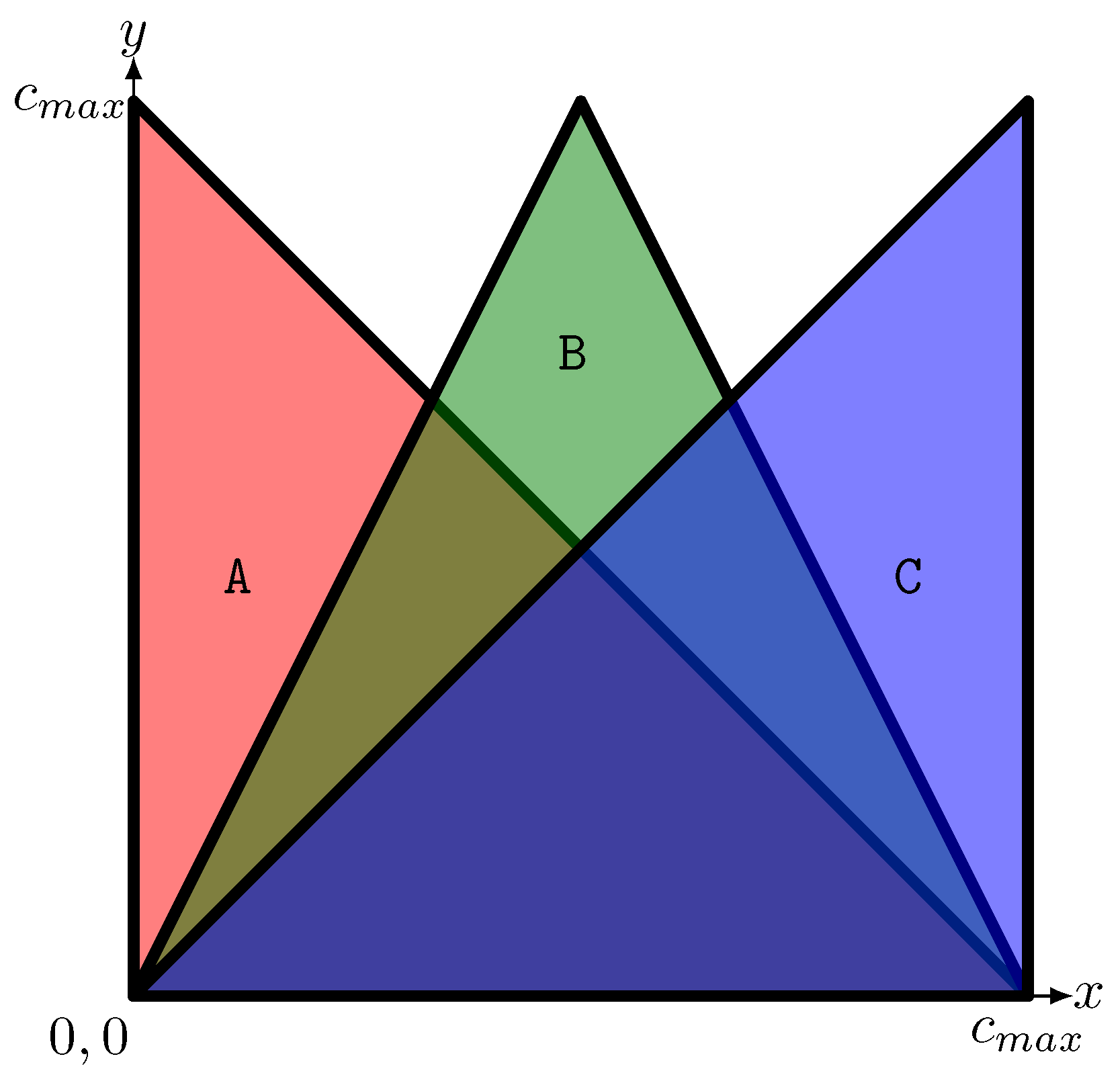
The geometric origin can be used to determine the maximum coordinate value for the determinants calculation. Figure 3 shows triangles which represent the set of all possible largest triangles within the positive integer coordinate range. The formula for calculating the triangle area (Equation (3)) makes it easy to deduce that all triangles have the same area.
Thus, the determinant can result in a maximum of twice the value (positive and negative) of the triangle area (Equation (4)). From this, Equation (5)) can be derived, by which the maximum possible coordinate value can be determined from the integer type used for the determinant calculation.
Now we have to consider how integer coordinates are calculated from the given coordinates (Equation (6)).
Equation (7)) illustrates that the size of the integer coordinates depends on the maximum extent and the maximum scale . If their product is larger than the maximum available coordinate value , data loss occurs because the coordinates are truncated by their remaining decimal places after scaling. The conversion is no longer bijective in this case.
If we use the 64 bit integer type for the determinant calculation, with a number range from to , we get
for the largest possible coordinate value. This number is greater than the maximum positive numerical value of 32 bit integers. Thus, they can be used for the coordinates. Assuming a necessary computational accuracy in the millimeter range (), the extent of an region must not be larger than 2,147,483.645 m, i.e., about 2000 km, in order to still calculate correctly with 32 bit integers. Thus, this range is only recommended for small-scale applications.
However, in order to be able to use the algorithm in all geospatial cases, it is advisable to work with 64 bit integers for the coordinates. This would even allow an extent of approx. 9,000,000,000,000 km with millimeter accuracy. Since the largest distance possible on Earth is approx. 40,000 km, 64 bit integers can map all coordinates up to a computational accuracy of 11 decimal places (10 pm). Thus, this number range is sufficient for all use cases in the GIS area. The disadvantage is that for the determinants 128 bit integers are needed, which are not always available natively in all programming languages or platforms.
After the conversion, the geometric features are stored with their integer coordinates, and a point set of all integer coordinates is formed (Figure 1b). During the generation of integer objects it must be checked that none of the features in is degenerated (Figure 4a) or if the orientation has changed (Figure 4b). A degeneration of a feature can be recognized by the fact that the end points of a line become congruent or it gets an area of zero, where a change of orientation is associated with a sign change of the area. In this case the feature must be discarded and cannot be analyzed with this method. For this reason, we use 64 bit integers. Alternatively, it is possible to decide based on the spatial extent (Equation (7)). Due to the previously explained usability of 64 bit integers, it can be assumed that degenerated features were already degenerated before the conversion.
3.3. Intersections as Rational Positions
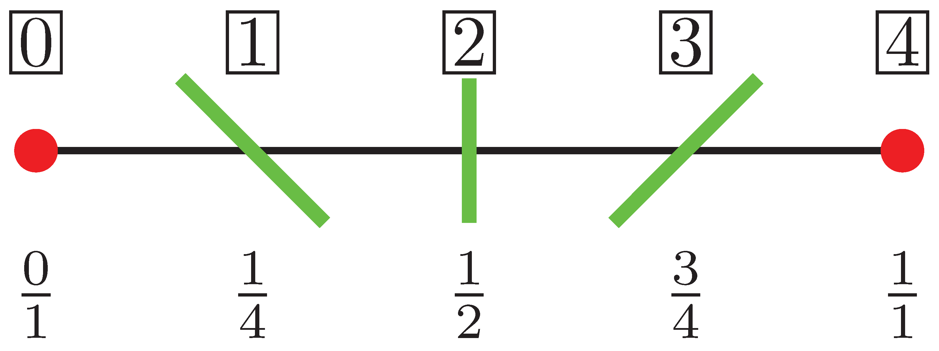
Integer numbers are used for the coordinates of in the basic mesh , but integer numbers cannot be used for intersection points, when reconstructing edges in , since intersection points are integer numbers only in exceptional cases. Even floating point numbers could not represent their positions correctly. Rational numbers are required.
We have decided not to calculate the intersection points as coordinates. We represent them as ordered positions on an edge (Figure 5) of the base mesh or a feature . However, this also requires rational numbers which are represented as a fraction of two integers. The given end points of the edges have integer values as coordinates. As a consequence, the position of the intersection point on these edges can be exactly expressed by a fraction of two integer values. This is true to all intersection points on an edge so that the order of these intersection points on an edge can be determined exactly as well.
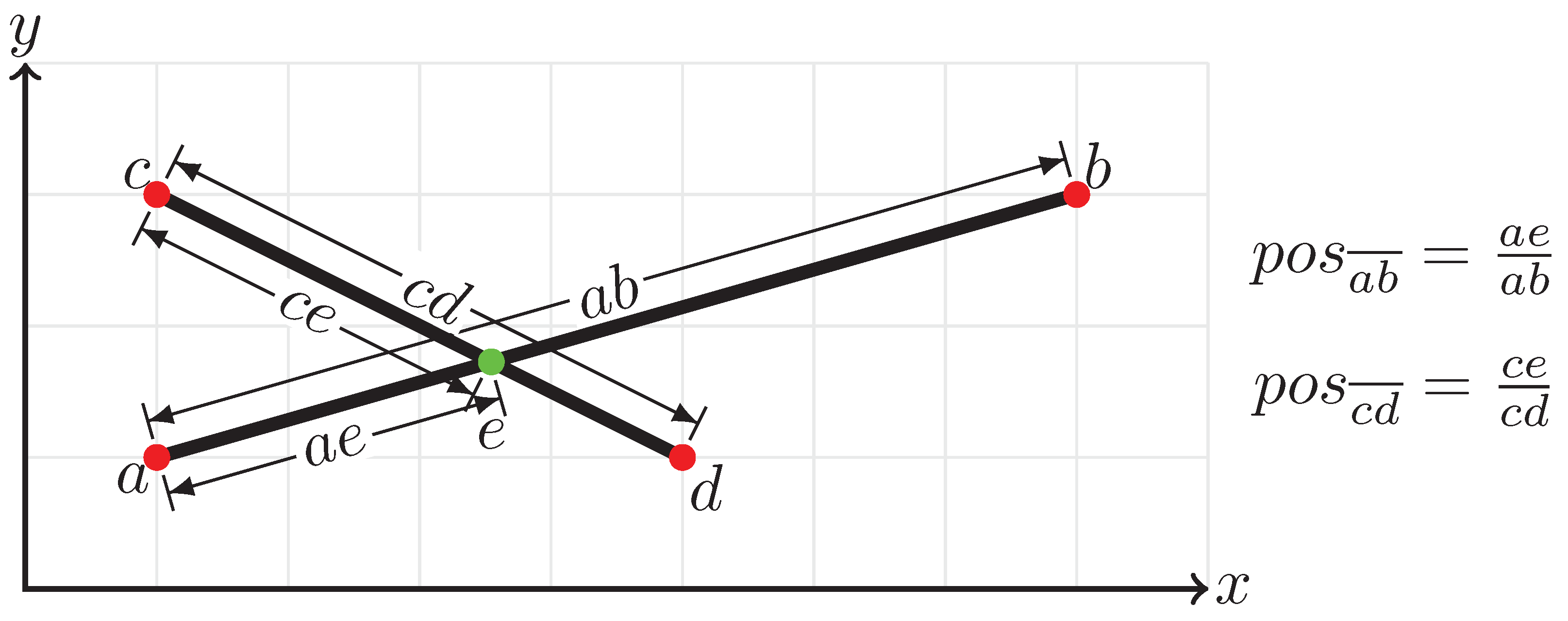
Equations (9) and (10) demonstrate how these positions can be calculated in the case of two intersecting edges ( and ). The values of and represent the relative position of the intersection point on the edges and . Thus the fractions are always in the range from 0–1.
Equation (11) shows an example for the position calculation, which is also depicted in Figure 6. Figure 6 also shows the geometric meaning of and , whose values were derived from the ratio of the partial distances to the total distances.
Since determinant calculations (similar to Equation (2)) are needed, the integer type resulting from this calculation (64 bit for 32 bit coordinates resp. 128 bit for 64 bit coordinates) must be used.
It is important to note that the coordinates of the intersection points are not required for our algorithm. The presented algorithm uses only relative positions on edges. However, absolute xy-coordinates can be calculated, for example, for display purposes. But the calculated xy-coordinates of the intersection points should not be used for further calculations, due to potential computational inconsistencies between geometry and topology.
3.4. Space Partition
The integer coordinates now form the basis of a Delaunay triangulation (Figure 1c). Theoretically, a simple triangulation would suffice, but it was proved in [18] that a Delaunay triangulation reduces the number of intersections. This triangulation provides the base mesh and remains structural unchanged in the next upcoming steps.
Then, successively the edges of the geometric features can be inserted into the base mesh (Figure 7). This step is subdivided into the following substeps:
- Since all points are already contained in the base mesh , the starting point of the edge has to be searched first (Figure 7a).
- Then the base mesh edge to the right of or on the feature edge is searched for (Figure 7b).If the feature edge lies on a base mesh edge , there are two possibilities. If the end point of the feature edge is identical to the end point of the base mesh edge , the loop for this edge is finished. Otherwise, the position of the endpoint of the base mesh edge on the feature edge is calculated and the loop jumps to item1 with this point as the new start point.Otherwise, go to the subsequent step with the next edge (in the triangle of the base mesh).
- The base mesh edge intersects the feature edge (Figure 7c), thus the positions of the intersection on both edges are calculated.Then, the opposite point in the neighboring triangle of the base mesh edge is determined and its location in relation to the feature edge is calculated.If the point is on the feature edge (Figure 7d), it is either the end point of the feature edge and this is finished. If it is not, the position on the feature edge will be calculated and with this point as new starting point jump to item 1.Otherwise, with the right respectively left base mesh edge this step (item 3) is processed again.
Once all sector triangle edges are inserted, the intersection points of these edges within the individual triangles of the basic mesh can be determined. The positions of the intersection points are stored as rational numbers as explained in Section 3.3.
In Figure 8 the individual steps for identifying edge intersections with within the triangles of are represented. For this purpose, an iteration is performed over the triangles of the base mesh. For each triangle the following substeps are processed:
- Determine all intersection points of feature edges on the triangle edge and sort counterclockwise around the triangle. (Figure 8a).
- Determine the inner intersection points according to the scheme in (Figure 8b). No geometric calculations are necessary for this. Intersections always result when the endpoint indices of one edge lie between the endpoint indices of the other edge.
- Calculate the intersection (again with rational numbers) position on both feature edges (Figure 8c).
All edges (basic mesh , geometric features ) and the positions of the intersections are then used to create half-edges(), which are then connected to form polygons (facets ).
Now each point (), each half-edge () and each facet () is checked to which geometric feature it belongs. Thereby an element can belong to none, one or more geometric features. Figure 9 shows how to find all elements of an areal geometric feature. First, all half-edges that lie on the boundary of the feature are determined (Figure 9a). The adjacent facets in the interior (Figure 9b) belong to the geometric feature. Then, the set of facets is extended by their neighboring facets until no new ones are found (Figure 9c). Finally, all points, half-edges and facets that were detected or are part of the detected elements are assigned to the feature.
At this stage we have a complete, gap-less and non-overlapping two-dimensional decomposition, generated fully automatically from the original data as seen in Figure 1.
3.5. Point, Line and Region Types
To increase the efficiency in using the space decomposition to determine the DE-9IM matrices, a preparation step is required.
The comparison to determine the DE-9IM matrices operates on three different types: Point, Line, and Region. They contain fields representing the set of Interior and Boundary elements (Table 3). The types indicate the geometric dimension of the geometric features to be represented.
- Dimension 0Point Points are objects without an extension. They have an inside (the point itself), no border and an outside (the rest). They can be derived directly from the OGC type Point and have only one Interior0 field, which consists of the vertex itself.
- Dimension 1Line Lines are line-shaped objects composed of one or more line segments. The interior of these objects are the edges of the line segments and the end vertices of the line segments that belong to multiple line segments. The boundary are the remaining end vertices. Objects without a boundary are also possible if the ring of line segments is closed. They are derived from the OGC types LineString and MultiLineString. Line objects have an Interior0 field with all end vertices that do not belong to the boundary, an Interior1 field with all half-edges, and a Boundary0 field with the associated end vertices.
- Dimension 2Region Regions are two-dimensional objects consisting of one or more facets. The interior consists of the regions between a closed ring of line segments. The boundary are all line segments and vertices of the object that are not inside. They are derived directly from the OGC type polygon. These objects have an Interior0 field with all vertices of the facets that are inside, an Interior1 field with all half-edges that are inside, and a 2-dimensional Interior field (Interior2) with the associated facets. Additionally, it has the Boundary1 field with the line segments that are not inside and a Boundary0 field with their end vertices.
Since in the last step of the spatial decomposition the elements of the base mesh were assigned to belong to a geometric feature, now the Point, Line and Region objects can be easily formed, depending on the OGC type of the associated features.
At this stage, the preparation for generating the DE-9IM matrices is complete. Only the generated Point, Line and Region objects with their associated elements are needed.
3.6. DE-9IM Matrices
With the now existing Point, Line and Region objects, one can easily determine the DE-9IM matrices. They have 0, 1, and 2 dimensional Interior (I) fields, and 0 and 1 dimensional Boundary (B) fields (Table 3). The Exterior (E) is made up of those elements that do not belong to the object.
In Equation (12) it can be seen how DE-9IM matrices are defined. The set operations of the definition can be applied directly to the previously created Point, Line and Region objects.
The operator can be implemented in such a way that it always returns the highest dimension that has a non-empty intersection between the comparison objects. The tests in the last column and row of the matrix have to be adapted, because the exterior is not stored directly. However, the tests can be easily adapted. Since we are working in a bounded region, the exterior is simply that part of the overall set which is not part of the interior and the boundary. Therefore, the types always have combined InteriorBoundary fields to allow easy querying (Table 3).
With this, the DE-9IM matrix can be easily created. If a simple binary 9IM matrix is needed, it can be easily converted. At all positions occupied by a 0, 1 or 2, a T (true) is set.
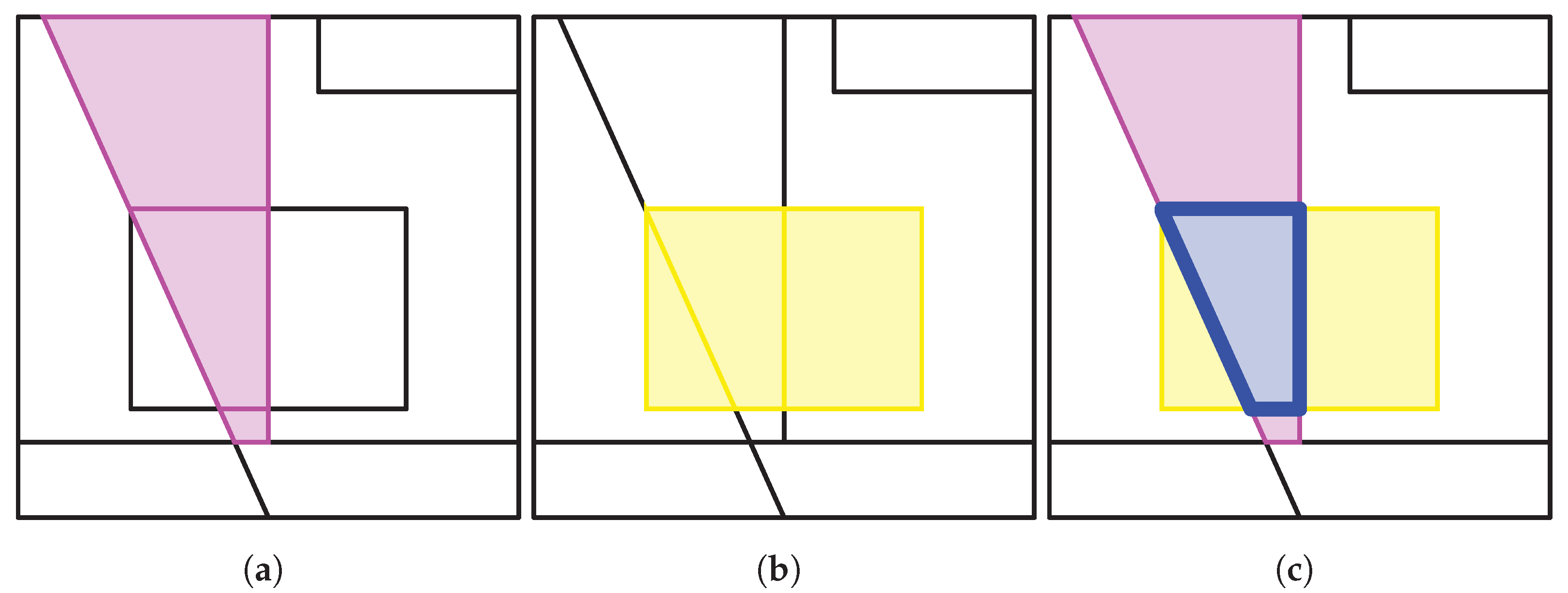
Figure 10 demonstrates how these set operations work. Figure 10a shows the region object of feature 2 in Figure 1a and Figure 10b shows the region object of feature A. Figure 10c then depicts the determined intersection. The DE-9IM matrix for this example is presented in Equation (13). In words, this is an overlaps relation. The individual cells of the matrix are created as shown in Table 4.
4. Results
The examples presented in this section investigate the application of the algorithm. They follow a specific test scenario. This test scenario is also conducted in established GIS tools. Then, the results are compared to demonstrate the capabilities of the presented approach. The test scenario was developed and tested in the context of a master’s thesis [19]. The rough test flow is represented in Figure 11 and will be presented in the following.
4.1. Examined Tools
A well-known opensource library for computing spatial predicates is the JTS Topology Suite (JTS) [1]. It implements the Simple Features Specification for SQL of OGC [20]. Since JTS can only work within a Java environment, there are also ports in other programming languages. A port to C++ is the GeometryEngine–OpenSource (GEOS) [21]. This port makes the functionality also usable by C/C++ tools. GEOS is for example used in the popular opensource spatial database PostGIS as well as in the opensource GIS tool QGIS. The NetTopologySuite (NTS) [22] is a direct port of the JTS targeting the .Net environment.
Since JTS and its ports are used so extensively, our algorithm is tested directly against this library respectively its port. Because of the ease of implementation in our used environment (Windows, .Net Framework) we have chosen NTS [22] and SpatiaLite (SpL.) [23]. The latter is a spatial database that is directly based on SQLite and can therefore run without a server installation.
These two tools are compared with the implementation of our algorithm. We use our algorithm in a version with 32 bit coordinates and a version with 64 bit coordinates. The 32 bit version is used to show possible problems with spatial tests in areas with large extent or high accuracy.
It is important that the tested tools meet the following conditions:
- Data transfer by using OGC WKT types.
- Test against a given DE-9IM matrix using the Relate method. (see [14], p. 17).
4.2. Test Design
The goal of the tests is to determine if any invalid results will be generated by the exanimated software tools. If so, it is further of interest for which geometric constellations (intersections) and (homeomorphic) variants the tests fail.
4.2.1. Tested Geometries
The three types Point, Line and Region have different properties (interior, exterior, boundary), so there are many possible combinations. For our tests, we decided to use the selection of combinations shown in Figure 12. This selection represents many different spatial relations and although it is only a subset of all possible combinations, it achieves many variations in the DE-9IM matrix. The figure shows combinations of Point with Point, Point with Line, Line with Line, Point with Region, Line with Region, and Region with Region.
The configuration of the tests was chosen to produce as many variations of DE-9IM matrices as possible. This is represented in Table 5.
It is important to mention, that not all possible relationships of features are covered in this document. Only cases in which different DE-9IM matrices occur. Tests with the reversed order of features are not represented in Table 5, but they are calculated and checked with every test. This is easily done because the DE-9IM matrix of the inverted comparison corresponds to the transposed original matrix.
The actual geometries of the objects are set to have integer coordinates. This results in a of 0 for the untransformed features. It guarantees that the base tests match the DE-9IM matrices represented in Table 5. The features themselves are stored as OGC WKT (see Table 6). The extent () of all test areas is not greater than 1056 so that all tested tools compute these base tests correctly.
Since the basic tests are designed in such a way that they should produce correct results with every tool to be tested, they cannot be used directly to point out problems with the tools. In the following it is shown how the features are changed by a homeomorphic mapping for the tests in such a way that the topology remains, but other coordinates are used in the computation. When creating the WKT features to be tested, care must be taken that no errors are produced just by the type of calculation. For this reason also decimal128 numbers are used. This avoids invalid test geometries due to number conversion when applying the homeomorphic mapping for the test cases.
After creating the transformed WKT features, all tools to be tested get them passed as a string.
4.2.2. Translation
A simple way to perform homeomorphic mapping is the translation. It transforms the coordinates of the base features as shown in Equation (14).
The values for T can be seen in Table 7. There are in total 60 different values. These are chosen so that, firstly, the number of decimal places increases from 1–6. Secondly, the integer part increases from 0 to 1,000,000 by a power of ten correspondingly.
In this way, coordinates up to an accuracy in the nanometer range are obtained during translation. Also region extents are obtained which are larger than the maximum possible distance on the earth’s surface (40,000 km). Thus, the tests should cover all GIS application areas.
An example of a translation of features shows Listing 1. The example uses test number 4.

Listing 1.
Test # 4 translated.
| Original (integer) |
| POINT(257 529) |
| LINESTRING(1 1, 513 1057) |
| Translation with 0.1 |
| POINT(257.1 529.1) |
| LINESTRING(1.1 1.1, 513.1 1057.1) |
| Translation with 100000000.000001 |
| POINT(100000257.000001 100000529.000001) |
| LINESTRING(100000001.000001 100000001.000001, 100000513.000001 100001057.000001) |
4.2.3. Scaling
Another simple homeomorphic mapping to perform is scaling. Point coordinates are scaled by the application of Equation (15) with a value .
The values for S in the tested examples are identical to the values for translation and can be seen in Table 7.
In the case of scaling, as well as in the case of translation, coordinates are obtained down to an accuracy in the nanometer range. In the case of scaling, the resulting range also covers all possible GIS application.
In Listing 2 the effect of scaling is represented by the example of the test number 4.
Listing 2.
Test # 4 scaled.
| Original (integer) |
| POINT(257 529) |
| LINESTRING(1 1, 513 1057) |
| Scaling with 0.1 |
| POINT(25.7 52.9) |
| LINESTRING(0.1 0.1, 51.3 105.7) |
| Scaling with 100000000.000001 |
| POINT(25700000000.000257 52900000000.000529) |
| LINESTRING(100000000.000001 100000000.000001, 51300000000.000513 105700000000.001057) |
4.3. Test Results
This section shows the results of the tests. Listing 3 shows the total number of tests which results from the number of comparison tests (33) and the number of translation and scaling values (60 each).
Table 8 demonstrates for which tests and for how many translation or scaling values the tested tools fail or calculate with data loss. Failure means that the test of the two features from Figure 12 resp. Table 5 with the Relate method of the tested tool responds with false to the given DE-9IM matrix (as well as to the transformed DE-9IM matrix in case of reversed).
Listing 3.
Test statistics.
| Number of Test Cases: 33 |
| Number of Translation Values: 60 |
| Number of Scaling Values: 60 |
| Total Number of unmodified Tests: 33 |
| Total Number of Translation Tests: 33 * 60 = 1980 |
| Total Number of Scaling Tests: 33 * 60 = 1980 |
| Total Number of Tests: 33 + 1980 + 1980 = 3993 |
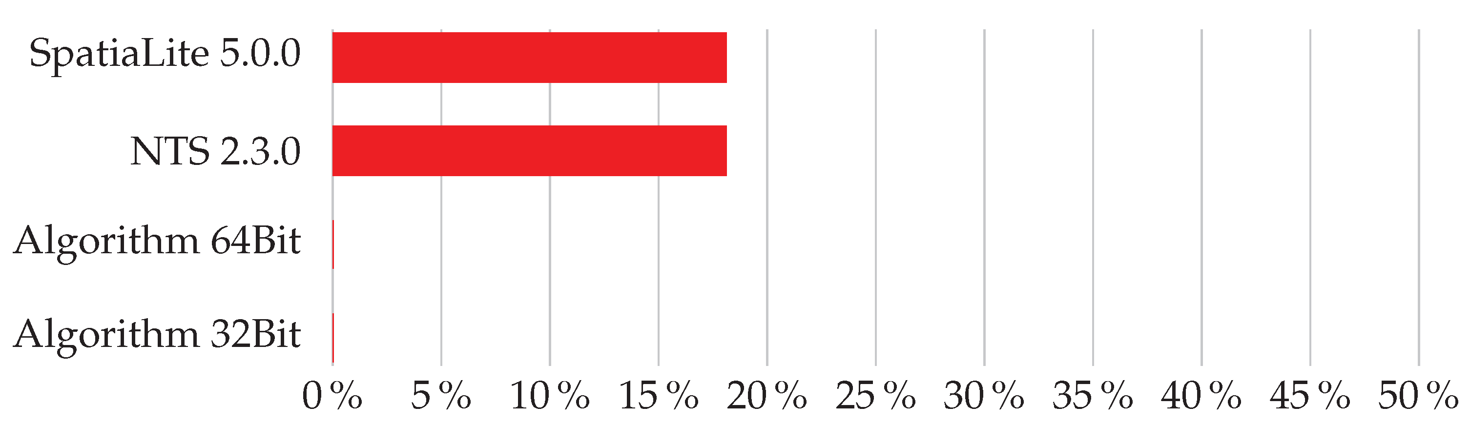
We can see that the translation has no influence on the result of our algorithm, because the translation does not change the maximum extent () of the test region. However, this is not the case for the other tools. They both fail with the same translation values and test cases, which refers to the identical computational kernel. It is significant that always such tests fail, which are based on a test “point on straight line” resp. “straight line collinear to straight line”.
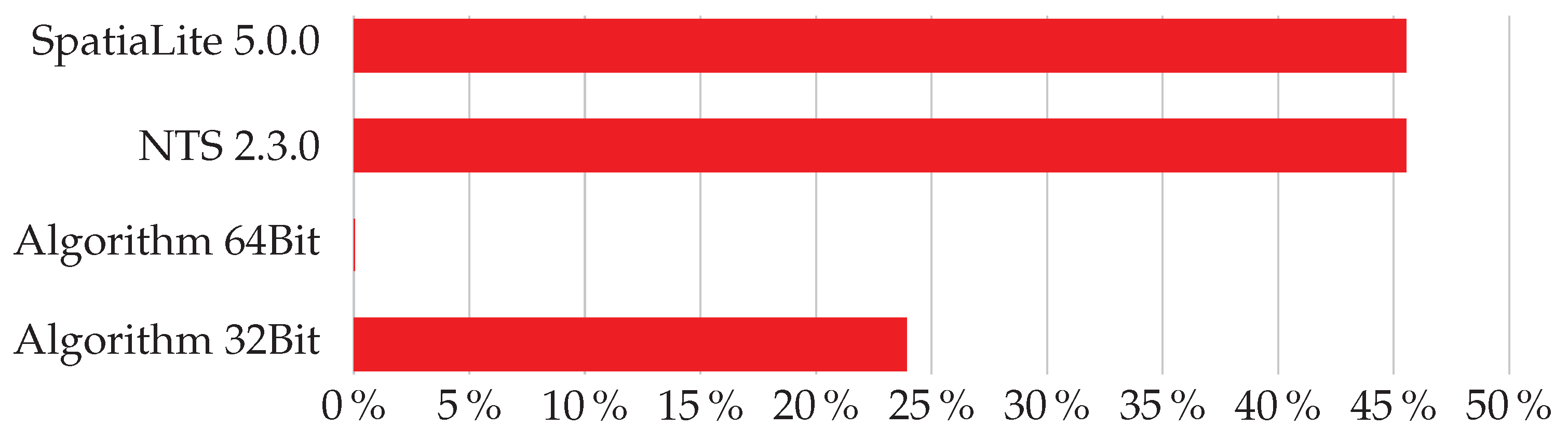
Similarly, it can be seen that our algorithm in the 32-bit version fails exactly the same tests as the other tools, because of the data loss in the integer conversion of the coordinates when the scaling factor is too large (). However, unlike the other tools, this could be accurately predicted beforehand with Equations (7). Similarly, our test in the 64 bit version exhibits the predicted behavior and does not fail in any of the transformation tests.
The behavior across all tests can be seen in Figure 13 and Figure 14. It can be clearly seen, that only our algorithm (64 bit) produces correct results. Other tools always produce unreliable results (at least as soon as “point to straight line” resp. “straight line collinear to straight line” tests are involved).
5. Discussion
As the presented tests proved, our novel approach offers a better alternative in determining spatial relations of geometric features.
The other two tested tools always failed when the tests involve “point on line” respectively “line collinear to line” tests. Both tools are based on the JTS. Therefore, it is not possible to determine whether the errors are due to the implementation or the use of floating point numbers. But as the examples in Table 2 show, this problem is fundamental since binary floating point numbers are not suitable for lossless representation of the digits after the decimal point.
In this context, the performance of our algorithm was not tested in relation to the other tools for a large amount of data since this is only a proof of concept. However, our algorithm should be at least used when the reliability of the results is important, regardless of the performance.
The initial claim was that our algorithm always produces correct results when comparing geometric features. Based on the tests, this was clearly proven for the algorithm with 64 bit integers. Although these tests do not cover all possible combinations and region extents, the proof in Section 3.2 shows that the possible region extent is perfectly sufficient for all GIS use cases. For smaller regions, the 32 bit implementation can also be used. This has the advantage that no 128 bit integers are required during the computation. In addition, it can be automatically identified whether the computation must be better accomplished with the 64 bit version, if a data loss is expected.
An important part of the presented approach is also the space decomposition from Section 3.4 because only this guarantees the correct functionality of the algorithm. In addition, this method of space decomposition has the advantage that, if it is used consistently for model generation, the consistency of topology and geometry can be guaranteed.
Another advantage of the presented approach is that the used Point, Line and Region types can also be used, for example, to easily generate the results of Boolean operations of two geometries.
All in all, our algorithm offers a real alternative to established methods in the comparison of geometric features and additionally has a great potential to extend the range of applications.
6. Outlook
The approach presented in this paper is restricted to the 2-dimensional space. It shows that the application of a space partitioning concept works and give results without topological inconsistencies. In a space partitioning concept, objects are not tested against each other with all well know problems of the fact that the computer cannot represent all real numbers.
It is a challenge to apply the concept of space partitioning to the 3-dimensional space. Two different ways can be applied: development of a theory and a tool which offers functionality to construct 3-dimensional space partitions from scratch and the transformation of existing boundary representations into a space partition. The first approach is under development [24]. The second approach is the basis of the research presented in this paper. Investigations of the application of this approach to the 3-dimensional space are also under development [25].
There are still challenges in this field. Research in the 3-dimensional space has the potential to close the gap between applications of GIS and digital buildings models in the field of Building Information Modeling. We accept these challenges and focus in our future collaboration on a next step to improve digital geometrical modeling.
Author Contributions
Conceptualization, Enrico Romanschek, Christian Clemen and Wolfgang Huhnt; Data curation, Enrico Romanschek; Formal analysis, Enrico Romanschek; Funding acquisition, Christian Clemen; Investigation, Enrico Romanschek; Methodology, Enrico Romanschek; Project administration, Christian Clemen and Wolfgang Huhnt; Resources, Christian Clemen; Software, Enrico Romanschek; Supervision, Christian Clemen and Wolfgang Huhnt; Validation, Enrico Romanschek; Visualization, Enrico Romanschek; Writing—original draft, Enrico Romanschek; Writing—review & editing, Enrico Romanschek, Christian Clemen and Wolfgang Huhnt. All authors have read and agreed to the published version of the manuscript.
Funding
This research was funded by the European Social Fund (ESF) and the Saxon State Ministry for Science, Culture and Tourism (SMWK), Funding No. 100343085. This Article is funded by the Open Access Publication Fund of Hochschule für Technik und Wirtschaft Dresden University of Applied Sciences and the Deutsche Forschungsgemeinschaft (DFG, German Research Foundation)—432908064.

Institutional Review Board Statement
Not applicable.
Informed Consent Statement
Not applicable.
Data Availability Statement
Source code for algorithm, source code for test suite, test data and test results are available at https://github.com/dd-bim/topology-relations.git (accessed on 19 October 2021).
Conflicts of Interest
The authors declare no conflict of interest.
Abbreviations
The following abbreviations are used in this manuscript:
| GIS | Geographic Information System |
| CAD | Computer Aided Design |
| 9IM | Nine Intersection Model |
| DE-9IM | Dimensionally Extended Nine Intersection Model |
| OGC | Open Geospatial Consortium |
| WKT | Well Known Text |
| JTS | JTS Topology Suite |
| NTS | Net Topology Suite |
References
- JTS Topology Suite. An API of Spatial Predicates and Functions for Processing Geometry. Available online: https://www.tsusiatsoftware.net/jts/main.html (accessed on 19 October 2021).
- Hoffmann, C. The problems of accuracy and robustness in geometric computation. Computer 1989, 22, 31–39. [Google Scholar] [CrossRef]
- Fortune, S.; Van Wyk, C.J. Static Analysis Yields Efficient Exact Integer Arithmetic for Computational Geometry. ACM Trans. Graph. 1996, 15, 223–248. [Google Scholar] [CrossRef]
- Shewchuk, J.R. Robust Adaptive Floating-Point Geometric Predicates. In Proceedings of the Twelfth Annual Symposium on Computational Geometry (SCG ’96), Philadelphia, PA, USA, 24–26 May 1996; Association for Computing Machinery: New York, NY, USA, 1996; pp. 141–150. [Google Scholar] [CrossRef]
- Yap, C.K. Towards exact geometric computation. Comput. Geom. 1997, 7, 3–23. [Google Scholar] [CrossRef] [Green Version]
- Thompson, R.J. Towards a Rigorous Logic for Spatial Data Representation; Nederlandse Commissie voor Geodesie (NCG): Delft, The Netherlands, 2007; Available online: http://www.gdmc.nl/projects/rgi-otb/3dtopo/documents/RGI-011-71.pdf (accessed on 19 October 2021).
- Sugihara, K.; Iri, M. A Solid Modelling System Free from Topological Inconsistency. J. Inf. Process. 1990, 12, 380–393. [Google Scholar]
- Huhnt, W. Reconstruction of edges in digital building models. Adv. Eng. Inform. 2018, 38, 474–487. [Google Scholar] [CrossRef]
- Giovanella, A.; Bradley, P.E.; Wursthorn, S. Evaluation of Topological Consistency in CityGML. ISPRS Int. J. Geo-Inf. 2019, 8, 278. [Google Scholar] [CrossRef] [Green Version]
- Jahn, M.W.; Bradley, P.E.; Al Doori, M.; Breunig, M. Topologically Consistent Models for Efficient Big Geo-Spatio-Temporal Data Distribution. ISPRS Ann. Photogramm. Remote Sens. Spatial Inf. Sci. 2017, IV-4/W5, 65–72. [Google Scholar] [CrossRef] [Green Version]
- Egenhofer, M. A mathematical framework for the definition of topological relations. In Proceedings of the Fourth International Symposium on Spatial Data Handing, Zurich, Switzerland, 23–27 July 1990; pp. 803–813. [Google Scholar]
- Egenhofer, M.J.; Sharma, J.; Mark, D.M. A critical comparison of the 4-intersection and 9-intersection models for spatial relations: Formal analysis. In Proceedings of the 11th International Symposium on Computer-Assisted Cartography, Minneapolis, MN, USA, 30 October–1 November 1993; pp. 1–11. [Google Scholar]
- Clementini, E.; Di Felice, P.; van Oosterom, P. A small set of formal topological relationships suitable for end-user interaction. In Advances in Spatial Databases; Abel, D., Chin Ooi, B., Eds.; Springer: Berlin/Heidelberg, Germany, 1993; pp. 277–295. [Google Scholar]
- OpenGIS® Implementation Standard for Geographic Information—Simple Feature Access—Part 1: Common Architecture; OpenGIS® Implementation Standard OGC 06-103r4; Open Geospatial Consortium Inc.: Rockville, MD, USA, 2011. Available online: https://portal.ogc.org/files/?artifact_id=25355 (accessed on 19 October 2021).
- Shen, J.; Zhou, T.; Chen, M. A 27-Intersection Model for Representing Detailed Topological Relations between Spatial Objects in Two-Dimensional Space. ISPRS Int. J. Geo-Inf. 2017, 6, 37. [Google Scholar] [CrossRef] [Green Version]
- Romanschek, E.; Clemen, C.; Huhnt, W. From Terrestrial Laser Scans to a Surface Model of a Building: Proof of Concept in 2D. In Proceedings of the EG-ICE 2020 Workshop on Intelligent Computing in Engineering, Online, 1–4 July 2020; Ungureanu, L.-C., Hartmann, T., Eds.; Universitätsverlag TU: Berlin, Germany, 2020; pp. 432–442. [Google Scholar] [CrossRef]
- IEEE Standard for Floating-Point Arithmetic. Standard IEEE 754-2019. In Proceedings of the C/MSC—Microprocessor Standards Committee, 2019. Available online: https://standards.ieee.org/standard/754-2019.html (accessed on 19 October 2021).
- Vetter, J. Eine Untersuchung zum Aufwand bei der Berechnung Einer Raumzerlegung im 2D aus Einer Gegebenen Menge an Polygonen. Master’s Thesis, Technische Universität, Berlin, Germany, 2019. [Google Scholar]
- Schönbrodt-Rühl, W. Semi-Automatisches Testbed zur Prüfung der Berechnung von Räumlich-Topologischen Prädikaten nach dem DE9IM Schema. Master’s Thesis, Hochschule für Technik und Wirtschaft, Dresden, Germany, 2021. [Google Scholar]
- OpenGIS® Implementation Standard for Geographic Information—Simple Feature Access—Part 2: SQL Option; OpenGIS® Implementation Standard OGC 06-104r4; Open Geospatial Consortium Inc.: Rockville, MD, USA, 2010; Available online: https://portal.ogc.org/files/?artifact_id=25354 (accessed on 19 October 2021).
- GEOS (GeometryEngine—OpenSource), a C++ Port of the JTS Topology Suite (JTS). Available online: https://trac.osgeo.org/geos/ (accessed on 19 October 2021).
- NetTopologySuite. A .NET GIS Solution That Is Fast and Reliable for the .NET Platform. NetTopologySuite Is a Direct-Port of All the Functionalities Offered by JTS Topology. Available online: https://nettopologysuite.github.io/NetTopologySuite/ (accessed on 19 October 2021).
- SpatiaLite Is an Open Source Library Intended to Extend the SQLite Core to Support Fully Fledged Spatial SQL Capabilities. Available online: https://www.gaia-gis.it/fossil/libspatialite/index (accessed on 19 October 2021).
- Galishnikova, V.; Huhnt, W. Polyhedral space partitioning as an alternative to component assembly. In ECPPM 2021—eWork and eBusiness in Architecture, Engineering and Construction—Proceedings of the 13th European Conference on Product & Process Modelling (ECPPM 2021), Moscow, Russia, 15–17 September 2021; CRC Press: London, UK, 2021. [Google Scholar]
- Vetter, J.; Huhnt, W. Accuracy Aspects when Transforming a Boundary Representation of Solids into a Tetrahedral Space Partition. In Proceedings of the EG-ICE 2021 Workshop on Intelligent Computing in Engineering, Hybrid, 30 June–2 July 2021; Abualdenien, J., Borrmann, A., Ungureanu, L.-C., Hartmann, T., Eds.; Universitätsverlag TU: Berlin, Germany, 2021; pp. 320–329. [Google Scholar] [CrossRef]
Figure 1.
Main steps from plan to spatial decomposition. (a) Regular site plan. (b) Points of all features in the plan. (c)Triangulation of all points. (base mesh) (d) Spatial decomposition of the plan.
Figure 1.
Main steps from plan to spatial decomposition. (a) Regular site plan. (b) Points of all features in the plan. (c)Triangulation of all points. (base mesh) (d) Spatial decomposition of the plan.

Figure 2.
Steps to prepare the geometric features.

Figure 3.
Triangles with maximum possible area.

Figure 4.
Changes due to the usage of integer coordinates instead of floating. (a) Degeneration. (b) Orientation.
Figure 4.
Changes due to the usage of integer coordinates instead of floating. (a) Degeneration. (b) Orientation.

Figure 5.
Intersection as fraction (multiple intersections on one edge).

Figure 6.
Intersection example of two edges.

Figure 7.
Reconstruction of feature edges. (a) Start point search. (b) Right most edge. (c) Next triangle edge. (d) Opposite point.
Figure 7.
Reconstruction of feature edges. (a) Start point search. (b) Right most edge. (c) Next triangle edge. (d) Opposite point.

Figure 8.
Intersections inside triangles (vertices and intersections on boundary indexed in order). (a) Crossing feature edges. (b) Selection by index. (c) Intersecting pair of edges.
Figure 8.
Intersections inside triangles (vertices and intersections on boundary indexed in order). (a) Crossing feature edges. (b) Selection by index. (c) Intersecting pair of edges.

Figure 9.
Assignment of facets to a feature. (a) Feature boundary detection. (b) Adjacent facets of the boundary edges. (c) Completed search.
Figure 9.
Assignment of facets to a feature. (a) Feature boundary detection. (b) Adjacent facets of the boundary edges. (c) Completed search.

Figure 10.
Intersection as set operation. (a) Parts of feature 2. (b) Parts of feature A. (c) Common Parts.
Figure 10.
Intersection as set operation. (a) Parts of feature 2. (b) Parts of feature A. (c) Common Parts.

Figure 11.
Test procedure in rough diagram form.

Figure 12.
Numbered test cases (simplified representation).

Figure 13.
Failed translations (percent of total 1980 tests).

Figure 14.
Failed scalings (percent of total 1980 tests).

Table 1.
Used OGC Simple Features and WKT representations.
| Simple Feature | WKT Example | Dim |
|---|---|---|
| Point | POINT(1 2) | 0 |
| LineString | LINESTRING(1 2, 5 5, 10.1 3.1) | 1 |
| Polygon | POLYGON((1 1, 5 1, 3 5, 1 1),(2 2, 3 2, 3 3, 2 2)) | 2 |
| MultiLineString | MULTILINESTRING((1 2, 5 5),(2 2, 3 2)) | 1 |
Table 2.
Examples for decimal to binary conversion and vice versa.
| Decimal | Binary | Decimal | ||
|---|---|---|---|---|
| → | → | |||
| → | → | |||
| → | → |
Table 3.
Used fields (marked with an “x”) of Point, Line and Region types.
| Field | Type | |||
|---|---|---|---|---|
| Name | Mesh Element | Point | Line | Region |
| Interior0 | Vertex | x | x | x |
| Interior1 | HalfEdge | x | x | |
| Interior2 | Facet | x | ||
| Boundary0 | Vertex | x | x | |
| Boundary1 | HalfEdge | x | ||
| InteriorBoundary0 | Vertex | x | x | x |
| InteriorBoundary1 | HalfEdge | x | ||
| Matrix (Equation (13)) | ||||
|---|---|---|---|---|
| Row | Col. | Val. | Definition | Calculation |
| 1 | 1 | 2 | ||
| 1 | 2 | 1 | ||
| 1 | 3 | 2 | ||
| 2 | 1 | 1 | ||
| 2 | 2 | 0 | ||
| 2 | 3 | 1 | ||
| 3 | 1 | 2 | ||
| 3 | 2 | 1 | ||
| 3 | 3 | 2 | is always 2, because the exteriors of | |
| objects would always overlap if the | ||||
| space is larger than the objects. | ||||
Table 5.
Test cases.
| Test # | Feature A | Feature B | DE-9IM Matrix |
|---|---|---|---|
| 1 | Point | Point | FF0FFF0F2 |
| 2 | Point | Point | 0FFFFFFF2 |
| 3 | Point | Line | FF0FFF102 |
| 4 | Point | Line | 0FFFFF102 |
| 5 | Point | Line | F0FFFF102 |
| 6 | Line | Line | FF1FF0102 |
| 7 | Line | Line | 1FFF0FFF2 |
| 8 | Line | Line | 101FF0FF2 |
| 9 | Line | Line | 101F00FF2 |
| 10 | Line | Line | FF10F0102 |
| 11 | Line | Line | 1010F0102 |
| 12 | Line | Line | FF1F00102 |
| 13 | Line | Line | 0F1FF0102 |
| 14 | Point | Region | FF0FFF212 |
| 15 | Point | Region | 0FFFFF212 |
| 16 | Point | Region | F0FFFF212 |
| 17 | Line, | Region | FF1FF0212 |
| 18 | Line | Region | 1FF0FF212 |
| 19 | Line | Region | FF1F00212 |
| 20 | Line | Region | 101F00212 |
| 21 | Line | Region | 1FF00F212 |
| 22 | Line | Region | F1FF0F212 |
| 23 | Line | Region | 1010F0212 |
| 24 | Line | Region | F11FF0212 |
| 25 | Line | Region | 101FF0212 |
| 26 | Region | Region | FF2FF1212 |
| 27 | Region | Region | 2FFF1FFF2 |
| 28 | Region | Region | 2FF1FF212 |
| 29 | Region | Region | FF2F01212 |
| 30 | Region | Region | FF2F11212 |
| 31 | Region | Region | 2FF10F212 |
| 32 | Region | Region | 212101212 |
| 33 | Region | Region | 2FF11F212 |
Table 6.
WKT Geometries of the first 10 tests.
| Test # | Geometry A | Geometry B |
|---|---|---|
| 1 | POINT(1 1) | POINT(1 2) |
| 2 | POINT(1 1) | POINT(1 1) |
| 3 | POINT(2 1) | LINESTRING(1 1, 513 1057) |
| 4 | POINT(257 529) | LINESTRING(1 1, 513 1057) |
| 5 | POINT(513 1057) | LINESTRING(1 1, 513 1057) |
| 6 | LINESTRING(682 623, 496 1104) | LINESTRING(1 1, 513 1057) |
| 7 | LINESTRING(1 1, 513 1057) | LINESTRING(1 1, 513 1057) |
| 8 | LINESTRING(1 1, 513 1057) | LINESTRING(353 727, 161 331) |
| 9 | LINESTRING(673 1387, 1 1) | LINESTRING(1 1, 513 1057) |
| 10 | LINESTRING(241 496, 297 604) | LINESTRING(1 1, 513 1057) |
Table 7.
Used values for scaling and translation (excerpt).
| # | Value |
|---|---|
| 1 | 0.1 |
| 2 | 0.01 |
| 3 | 0.001 |
| 4 | 0.0001 |
| 5 | 0.00001 |
| 6 | 0.000001 |
| 7 | 1.1 |
| 8 | 1.01 |
| ⋮ | ⋮ |
| 59 | 100,000,000.00001 |
| 60 | 100,000,000.000001 |
Table 8.
Results after translation (T) and scaling (S) according to test cases.
| All Passed: √, Passed Despite Data Loss: (√), Failed: Percent of Tests | ||||||||
|---|---|---|---|---|---|---|---|---|
| Test | 32 bit a | 64 bit b | NTS c | SpL. d | ||||
| # | T | S | T | S | T | S | T | S |
| 1 | √ | (√) | √ | √ | √ | √ | √ | √ |
| 2 | √ | √ | √ | √ | √ | √ | √ | √ |
| 3 | √ | (√) | √ | √ | √ | √ | √ | √ |
| 4 | √ | 55 | √ | √ | 50 | 100 | 50 | 100 |
| 5 | √ | (√) | √ | √ | √ | √ | √ | √ |
| 6 | √ | (√) | √ | √ | √ | √ | √ | √ |
| 7 | √ | (√) | √ | √ | √ | √ | √ | √ |
| 8 | √ | 55 | √ | √ | 50 | 100 | 50 | 100 |
| 9 | √ | 55 | √ | √ | 50 | 100 | 50 | 100 |
| 10 | √ | 55 | √ | √ | 50 | 100 | 50 | 100 |
| 11 | √ | 55 | √ | √ | 50 | 100 | 50 | 100 |
| 12 | √ | (√) | √ | √ | √ | √ | √ | √ |
| 13 | √ | (√) | √ | √ | √ | √ | √ | √ |
| 14 | √ | (√) | √ | √ | √ | √ | √ | √ |
| 15 | √ | (√) | √ | √ | √ | √ | √ | √ |
| 16 | √ | 55 | √ | √ | 30 | 100 | 30 | 100 |
| 17 | √ | (√) | √ | √ | √ | √ | √ | √ |
| 18 | √ | (√) | √ | √ | √ | √ | √ | √ |
| 19 | √ | 55 | √ | √ | 30 | 100 | 30 | 100 |
| 20 | √ | 55 | √ | √ | 42 | 100 | 42 | 100 |
| 21 | √ | 18 | √ | √ | 42 | 100 | 42 | 100 |
| 22 | √ | 55 | √ | √ | 30 | 100 | 30 | 100 |
| 23 | √ | (√) | √ | √ | √ | √ | √ | √ |
| 24 | √ | 55 | √ | √ | 42 | 100 | 42 | 100 |
| 25 | √ | (√) | √ | √ | √ | √ | √ | √ |
| 26 | √ | (√) | √ | √ | √ | √ | √ | √ |
| 27 | √ | (√) | √ | √ | √ | √ | √ | √ |
| 28 | √ | (√) | √ | √ | √ | √ | √ | √ |
| 29 | √ | 55 | √ | √ | 30 | 100 | 30 | 100 |
| 30 | √ | 55 | √ | √ | 30 | 100 | 30 | 100 |
| 31 | √ | 55 | √ | √ | 42 | 100 | 42 | 100 |
| 32 | √ | (√) | √ | √ | √ | √ | √ | √ |
| 33 | √ | 55 | √ | √ | 30 | 100 | 30 | 100 |
a Our algorithm with 32 bit coordinates. b Our algorithm with 64 bit coordinates. c NetTopologySuite (NTS) 2.3.0. d SpatiaLite 5.0.0.
Publisher’s Note: MDPI stays neutral with regard to jurisdictional claims in published maps and institutional affiliations. |
© 2021 by the authors. Licensee MDPI, Basel, Switzerland. This article is an open access article distributed under the terms and conditions of the Creative Commons Attribution (CC BY) license (https://creativecommons.org/licenses/by/4.0/).
Share and Cite
MDPI and ACS Style
Romanschek, E.; Clemen, C.; Huhnt, W. A Novel Robust Approach for Computing DE-9IM Matrices Based on Space Partition and Integer Coordinates. ISPRS Int. J. Geo-Inf. 2021, 10, 715. https://doi.org/10.3390/ijgi10110715
AMA Style
Romanschek E, Clemen C, Huhnt W. A Novel Robust Approach for Computing DE-9IM Matrices Based on Space Partition and Integer Coordinates. ISPRS International Journal of Geo-Information. 2021; 10(11):715. https://doi.org/10.3390/ijgi10110715
Chicago/Turabian StyleRomanschek, Enrico, Christian Clemen, and Wolfgang Huhnt. 2021. "A Novel Robust Approach for Computing DE-9IM Matrices Based on Space Partition and Integer Coordinates" ISPRS International Journal of Geo-Information 10, no. 11: 715. https://doi.org/10.3390/ijgi10110715
Note that from the first issue of 2016, this journal uses article numbers instead of page numbers. See further details here.