Acoustic Pressure Pipette Aspiration Method Combined with Finite Element Analysis for Isotropic Materials


1
Institute of Measurement and Sensor Technology, UMIT—Private University for Health Sciences, Medical Informatics and Technology, 6060 Hall in Tirol, Austria
2
Division of Phoniatrics and Pediatric Audiology, Department of Otorhinolaryngology—Head and Neck Surgery, University Hospital Erlangen Medical School, Friedrich-Alexander-University Erlangen-Nürnberg, 91054 Erlangen, Germany
*
Author to whom correspondence should be addressed.
Appl. Sci. 2019, 9(18), 3875; https://doi.org/10.3390/app9183875
Submission received: 15 August 2019
/
Revised: 6 September 2019
/
Accepted: 7 September 2019
/
Published: 15 September 2019
(This article belongs to the Special Issue Computational Methods and Engineering Solutions to Voice)
Abstract
:A measurement setup combined with a numerical simulation by a linear finite element analysis is presented as a method to determine the elastic modulus of both artificial and real tissue as a function of frequency. At the end, the future goal is to develop and validate the method to measure the elastic modulus of in-vivo human vocal folds over the human phonation frequency range. In the present study, a miniaturized acoustic pressure pipette aspiration technique is developed to measure the material characteristics of an isotropic silicone specimen with similar characteristics as human vocal folds. In previous studies, friction and compression force effects of the pipette tip wall on the surface of the sample and the radius of the pipette were not investigated. Moreover, the large scale of the measurement setups made them impossible to use for clinical applications. Therefore, two different pipette sample cross-section boundary conditions and two different pipette radii were used. With the aim of ensuring reliable results, we tested our method with pipettes of two different radii on four silicone samples with different consistencies over a frequency range of 50–500 Hz. The simulation verified the measurement results in which the strong dependency of the elastic modulus on the excitation frequency, radius of the pipette, the pipette tip compression force and friction was revealed. By the simulation results, two different frequency dependent equations were developed for calculating elastic modulus of the silicone mixtures in the two cross-section boundary conditions. It was concluded that using a very small gap in between the pipette tip and the specimen can cancel the impact of the pipette tip force and friction which are the major cause of uncertainty. However, if a connection between the pipette and the surface is unpreventable, the contact force should be restricted to be absolutely zero.
1. Introduction
Today, developing new medical methods for preventing and treating voice disorders have high relevance. Those could improve the ability of early diagnosis e.g., in the case of cancer occur and eventually could help faster treatment and rehabilitation of patients. The vocal folds are the main organ in human voice production, the vocal folds’ sound emission is the major interest of many investigations in this area [1,2,3,4,5,6,7,8,9,10,11,12,13,14,15]. The determination of mechanical properties of synthetic as well as natural vocal fold material is an important task for further understanding of the phonation process. Consequently, numerous studies [16,17,18,19,20,21] have been focused on the analysis and development of synthetic vocal folds. In particular, silicone or polyurethane mixtures are used to produce vocal fold models [20,22,23,24], which is the target of the research of this study. This work presents a method to measure the elastic modulus of four silicone rubber samples with different stiffness ratios as a function of frequency similar to the vocal fold tissue that exhibits frequency-dependent parameters [25]. Our focus is on the pipette aspiration method that was originally introduced by Rand and Burton [26] to measure the stiffness and intracellular pressure of red blood cell membranes. Therein, a pipette was placed on the sample and, via a static low pressure, the sample surface was sucked into the pipette. A related method using a suction cup tool was used to measure the skins’ biaxial membrane properties [27]. The pipette aspiration method was later improved for a cultured cell treating application [28,29]. This method was improved upon more by Evans [30]. The pipette aspiration method application for estimating the elastic modulus of soft tissues was presented in [31,32]. Aoki et al. [33] applied it to a local elasticity measurement of soft tissue and a simple equation developed to calculate the static elastic modulus of the tissue. In his measurement setup, the soft tissue floated in a salt bath to counteract the compression force of the pipette tip on the sample surface. The equation was developed for a static measurement setup while the vocal folds’ modulus of elasticity is a function of frequency. Therefore, a lack of dependency of the equation terms on the excitation frequency and absence of the pipette wall force and friction influence on the vibrational behavior of the sample surface can be seen in the equation. Although, frequency-dependent analyses in a range of 0 Hz to 50 Hz have been done by previous studies [33,34,35,36,37] to investigate the local elastic modulus of real and synthetic vocal fold tissue. However, the examined range is not wide enough to cover the human speech sound frequency [38].
A frequency-dependent analysis in the frequency range of human phonation using the pipette aspiration method was first presented by Zörner et al. [39]. In the suggested setup, the silicone sample was placed under the pipette and it was lowered onto the sample taking special care that the pipette does not act any force onto the silicone, which would affect the results. By means of a pistonphone that was mounted on an electromechanical shaker, a fluctuating pressure was generated within the pipette. The out-of-plane velocity at the centre of the specimen’s surface within the pipette was measured by a laser scanning vibrometer. Weiss et al. [40,41,42] enhanced the setup of Zörner et al. [39] to suggest a reliable pipette aspiration method for spatially-resolved material characterization of synthetic vocal folds over a frequency range of 50 Hz to 700 Hz. Unlike the Aoki et al. [33] method to counteract the pipette wall force on the sample surface, Weiss et al. [40] limited the force to 0.1 N for all the mixtures in the frequency range. However, those measurement setups are not accurate enough to measure frequency-dependent material properties of anisotropic and inhomogeneous materials as existent in vocal folds. The first study [39] used the Aoki et al. [33] analytical approximation (see Equation (1)) to calculate the modulus of elasticity, which was developed for a static measurement; thus, it does not take into account all the impact factors of a dynamic measurement setup. The main drawback of the previous studies [39,40] is the large scale of the experimental setup that is not appropriate for a clinical use, which is the long-term goal of research in this area. Therefore, those tasks will be addressed with innovative measurement setups within this present study.
We enhanced the pipette aspiration method to a miniaturized size suitable for clinical use which allows applying an acoustic excitation on the surface of the sample at predefined frequencies in the human phonation range. We combined the experimental study with a numerical simulation to determine the capability of the present method for characterization of the frequency-dependent material properties of the silicone rubber mixtures and real vocal fold tissue. To investigate the influence of the pipette tip wall’s friction, force and radius on the vibrations behaviour of the sample surface enclosed by the pipette, the measurements and the simulation were conducted under two boundary conditions using two different pipette radii. In the first boundary condition, the pipette was connected to the surface and, in the second, was placed on the surface with a very small gap. The numerical simulation has made it possible to have a closer look at the behaviour of the surface under the pipette, which leads to developing two different frequency-dependent analytical approximations for calculating the elastic modulus of silicone sample in the two boundary conditions.
2. Material and Specimens
Silicone rubber is usually used for fabricating artificial models of human vocal folds because of the similar flexibility [19,43]. For experimental investigations, four mixing ratio samples 1:1:0, 1:1:2, 1:1:3 and 1:1:4 were made of a two-component silicone rubber Ecoflex 0030 (Smooth-On Inc., Macungie, PA, USA) exactly as in [44,45]. The stiffness of the cured silicone was adjusted by adding a variable amount of silicone thinner to the same amounts of the main components. The elasticity of the sample depends on the silicone thinner rate, so the higher amount of the thinner makes the silicone softer. Thus, a silicone mixture is named 1:1:x with x denoting the thinner amount related to the number of sub-components. The mixtures were moulded in cubic shape in 50 mm × 50 mm × 10 mm dimension. Simple geometry of the specimen was used to explore the isotropic material properties of the silicone rubber. These symmetric specimens can be fabricated easily and computing the finite element models is much shorter.
3. Experimental Setup
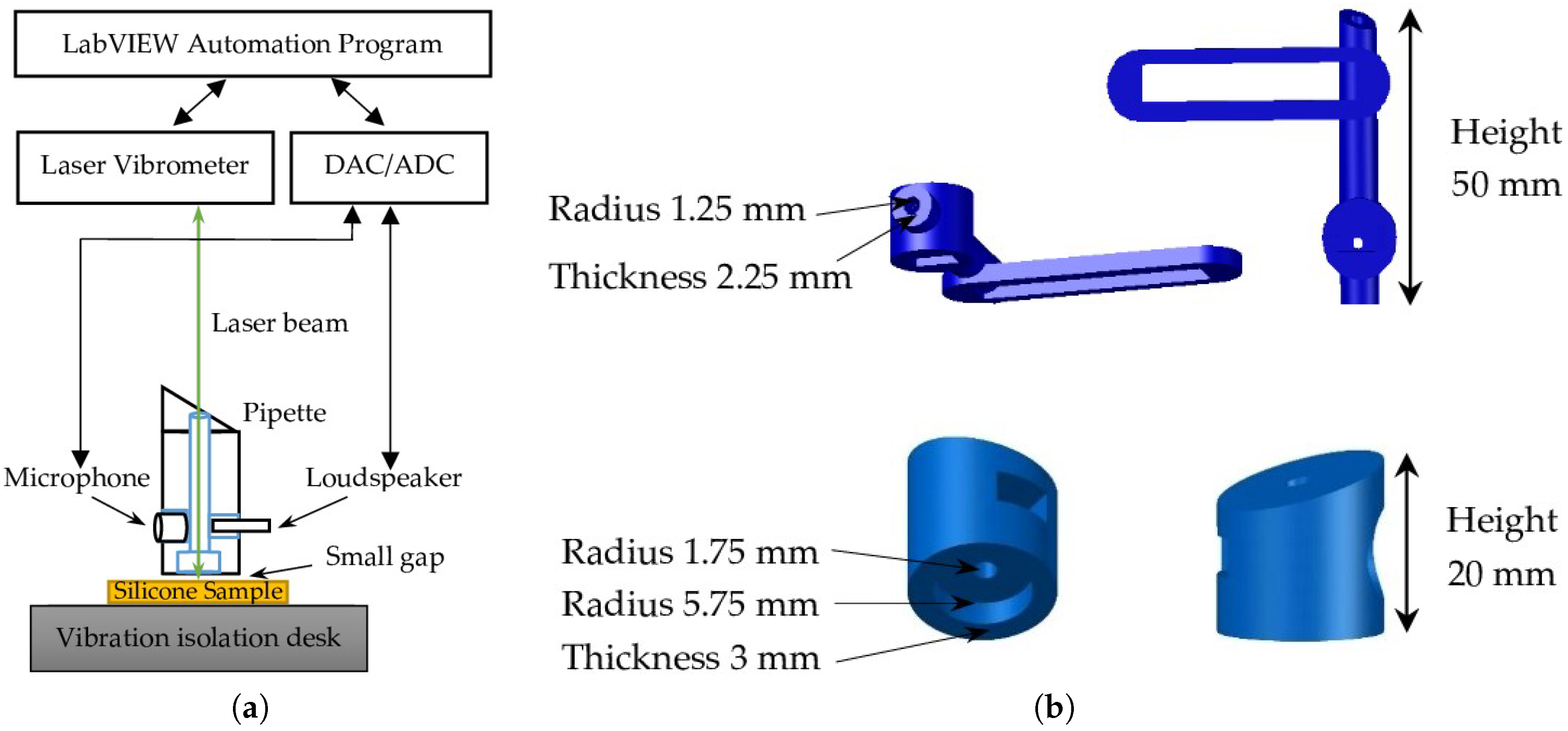
The measurement of the four samples was performed by the pipette aspiration method with the experimental setup shown in Figure 1. In the original setup as reported in Aoki et al. [33], a static low pressure was used to suck the material into the pipette and the resulting deformation was measured. The elastic modulus was determined by a simple analytical approximation (1). We improved the setup by using a miniaturised loudspeaker as a replacement for the pistonphone, which was used by Zörner et al. and Weiss et al. [39,40], in order to produce an acoustic pressure at predefined frequencies inside the pipette.
The bottom end of the pipette was placed on the surface of the sample perpendicularly in the two different contact boundary conditions. Firstly, the pipette was connected to the surface with imposing various amounts of force on it. In this condition, the sample surface under the pipette wall (in an area of a ring with a pipette radius) is completely restricted in the z-direction, but it may have movement in the x–y plane. Secondly, the pipette was placed on the sample surface with a very small gap in the range of tens of micrometers. It is obvious that, in this condition, the sample surface under the pipette wall is not under any constraint and it is free to move in all the directions. We call those two setups as connected pipette and pipette with a gap. The two boundary conditions help to investigate the effect of the pipette wall’s friction, force and radius on the behaviour of the surface under the fluctuating. Due to the sinusoidal sound excitation pressure within the pipette, the surface area aspires into the pipette wall and pushes in the negative z-direction as it is depicted in Figure 2b. The displacement amplitude (L) at the center of the pipette obtained from the velocity of the vibration is optically measured by means of the vibrometer as a function of the excitation pressure . In this study, we assumed that the silicone samples are isotropic and homogenous and have linear elasticity:
Based on those assumptions, the analytical approximation (1) taken from Aoki et al. [33] is used to calculate elastic modulus (E) of the samples using the pipette aspiration method. The coefficient (C) is corresponding to the effect of the pipette wall thickness (b/a), specimen thickness (h/a) and specimen radius (R/a) with respect to the pipette radius. A schematic of the pipette aspiration method and the sample deformation under the pipette are depicted in Figure 2. Since we used two different sizes of pipette, the coefficient was considered to be 1 for the smaller pipette and 1.1 for the bigger pipette; both are extracted from Aoki et al. [33]. By means of a transient mount, the distance between the pipette tip and the sample surface adjusted to implement the pipette with a gap boundary condition as displayed in Figure 1a. An accurate scale in tens of milli-Newton measuring range was added to the experimental setup to control the compression force of the pipette tip wall on the surface in connected pipette condition. A larger pipette with a bigger radius, 5.75 mm, was utilized in the experimental setup as shown in Figure 1b.
A tiny loudspeaker (Knowles Electronics LLC, Itasca, IL, USA) is mounted in a 10 mm distance from the base of the pipette. The sound excitation pressure inside the pipette obtained by the loudspeaker was driven at ten frequency steps in the range of 50 Hz–500 Hz with 50 Hz intervals to cover the normal vocal fold oscillation frequency range. The acoustic pressure applied to the inner volume of the pipette enables having an enclosed excitation pressure on the surface of the silicone sample. Thereby, the excitation pressure on the sample surface was measured by a microphone (CUI Inc., Tualatin, OR, USA) and the generated mechanical vibration by a laser vibrometer. Since the acoustic wavelengths are in the range of 0.686 m to 6.86 m and the radius of the both pipettes are in a few millimeter range, the pressure is constant in all the pipette volume. Therefore, the excitation pressure on the surface of the sample is equal to the pressure measured by the microphone that is placed in the pipette wall in front of the loudspeaker. The sound pressure received by the microphone is assigned to the pressure in Equation (1) to calculate the modulus of elasticity.
The amplitude of the surface vibration is in the range of a few micrometers, which demands a very accurate measurement method. Therefore, the OVF-5000 Xtra (Polytec GmbH, Waldbronn, Germany) is the newest Polytec modular laser vibrometer employed. A helium-neon laser exploits the Doppler Effect [46] to derive the velocity and the displacement obtained by integrating over the velocity, which is done by a LabVIEW automation program (LabVIEW NXG 3.1, National Instruments, Austin, TX, USA). A sketch of the whole setup is depicted in Figure 3a. To minimize the external influences, the experimental setup was placed on a vibration isolation desk for damping the external vibrations. Moreover, the other environmental factors like room vibrations, temperature, noise and humidity should be controlled to get precise results. The measurement in this study had been done at normal room temperature and humidity and the ground vibration and room noises had been kept as small as possible. The laser reflectability of the sample surface is low, making the measurement difficult; therefore, a titanium dioxide spray Ardrox® 9VF2 (Chemetall GmbH, Frankfurt am Main, Germany) was sprayed on the samples to reflect the laser light better. Since the coating is very fine, the elastic modulus is not influenced by it.
4. Numerical Simulation
A numerical simulation by a finite element method like in previous studies [47,48,49,50,51,52,53] was performed by a simplified model of the experimental setup. The numerical simulation modeled the 1:1:2 mixture as an example among the four mixtures. Therefore, damping ratio, Poisson’s ratio and density of the mixture are extracted from previous studies [44,45,54,55] and assigned to the model material content. The two following tasks were defined for the simulation. The first task was determining a frequency-dependent Young’s modulus of the model to investigate the capability of the present setup for characterization of the dynamic mechanical properties of the silicone rubber and vocal fold tissue—moreover, investigating possible limitations of the analytical approximation (1) for calculating the frequency-dependent modulus of elasticity, which was originally developed to calculate the static modulus of elasticity. The second task was examining the influence of the pipette-sample boundary condition, pipette tip compression force and the radius of the pipette, whose effects were detected in the measurement. This information helps to improve Equation (1) to be used in the two boundary conditions, while taking into account all the impact factors.
The Young’s modulus of the model is the criterion to be considered as the true value of the sample modulus of elasticity. Therefore, the first task could be obtained by comparing Young’s modulus of the model with the calculated modulus of elasticity from the measurement, at each of the excitation frequencies in the frequency range. To make the Young’s modulus and the calculated modulus of elasticity comparable, the predictions from the numerical of the model should be matched with the measured displacement by adjusting the model Young’s modulus when the measured pressure applied to the boundary . This process will be explained more in Section 4.3.
In the homogeneous computation, a three-dimensional finite element model was defined based on the experimental setup. Since a cubic or cylinder shape of the model in the same dimensions do not affect the results, to reduce the calculation time, an axisymmetric two-dimensional model was created from the -plane cross-section of the 3D model. The z-axis in the centre of the pipette in the 3D model is the symmetric axis (r) of the 2D model. With displacement simulated in the 2D and 3D models with the same situation, the results show a difference in range of a few nanometers, which is negligible in comparison with the huge difference in the computation time of the two models. Our explanation in this article is based on the 3D model to have a better understanding of the model behaviour in the simulation while all the simulation results were obtained from the 2D model.
The models were prepared and the computations were done using COMSOL Multiphysics (5.4, COMSOL Inc., Stockholm, Sweden) which is a simulation software currently being used for a wide range of applications worldwide. A hollow cylinder with inner radius 1.25 mm and outer radius of 2.25 mm and 1 mm height assumed as the pipette and it was placed on the centre of the upper surface of a cubic in 50 mm × 50 mm × 10 mm dimension identical to the experimental setup. Figure 4 shows the 2D and 3D models’ geometry. In the simulation, two different boundary conditions were defined to investigate the effects of the pipette cross-section friction with the specimen surface.
First, the bottom end of the pipette (cylinder) perpendicularly placed on the model top surface, restricted in the z-direction but free to move in another axis to simulate the situation where the pipette is connected to the sample. To model the 100 mN force which the pipette imposes on the silicone surface in the experimental setup, the 100 mN boundary load was assigned to the cross-section in the z-direction. Second, to model the gap between the tip of the pipette and the sample surface, the cross-section boundary was made free to move in all directions without any friction with the model surface.
Grid size: Extremely fine mesh was used in both 3D and 2D models to achieve a high resolution in the results. The 3D model was meshed by 504 edge elements, 17,254 boundary elements and 425,972 elements in total for the whole model. The maximum element size is 1 mm and 0.01 mm is the size of its smallest grid in the 3D model. While the 2D model was meshed by 280 edge elements and by 10,036 elements in total, the maximum element size in the 2D model is 0.25 mm and 0.5 μm is the size of its smallest grid. The models’ grid sizes should be extremely fine with considering the model dimensions and the generated displacement range, which is in the range of a few micrometres.
4.1. Stiffness
The mechanical behaviour of the model described by the Navier’s Equation (2). denotes the Cauchy stress, the density of the medium and u the mechanical displacement. All of the equations in this section are extracted from Kaltenbacher [56] (pp. 93–114):
Introducing the differential operator B:
The linear law of elasticity known as Hook’s law [57,58] is the commonly used relation between the stress and strain. The tensor of elasticity moduli [c], linear strain tensor [S] and tensor of the Cauchy stress introduced to express the relation in form (3):
and the linear strain tensor [S] can be expressed by:
4.2. Boundary Condition
Four types of boundary conditions, , , , , were defined in the model for different surfaces as shown in Figure 4. The is the boundary of the model surface inside the pipette, the corresponds to the pipette surface cross-section boundary condition, is the boundary of the bottom side of the model and all the other boundaries are shown with . The amplitude of the measured pressure applied to the boundary in which the pipette wall surrounds the surface. The relation (6) denotes the Cauchy stress tensor on the boundary . The Cauchy stress tensor is a function of representing the excitation pressure on the surrounded area:
Numerical simulation is conducted under the two following approaches regarding the pipette-sample connection condition. First, the boundary , which corresponds to the cross-section of the pipette tip wall and the surface of the sample, is restricted in the z-direction but free to move in the x–y plane. This boundary condition is called connected pipette (the pipette touches the surface) in this paper:
The 100 mN constant load in the z-direction is assigned to the boundary to reproduce the case in the experimental setup in which the pipette applies force on the silicone surface. represents the 100 mN constant contact force:
Second, the is free to move in the x–y–z plane to model the gap in the experimental setup. We will call this boundary condition a pipette with the gap condition in this paper:
Model movement is completely restricted leaving no degree of freedom from the bottom side:
All the other boundaries () are free in all directions; therefore, homogeneous edge conditions are applied:
Based on Equation (5), the dynamics of a single degree freedom systems with viscous damping are described by the following equation of motion in matrix form:
In Equation (8), u is the discrete displacement, M is the mass matrix and K denotes the stiffness matrix. The excitation force per unit area enters the equation by the term f on the right-hand side.
Damping: the damping of the linear elastic model is introduced via the Rayleigh damping in the simulation (see e.g., [56,59,60]). Since we will just consider steady-state vibrations and not any transient behaviour, Rayleigh damping is a simple way of generating a damping matrix as a pure linear combination of the mass and stiffness matrices. The damping can be added to Equation (8) by introducing damping matrix C. The damping matrix consists of mass matrix M and the stiffness matrix K. In Equation (9), denotes the mass proportional and the stiffness proportional damping coefficients, giving:
Equation (10) made by combining the matrix (9) into Equation (8) which numerical simulation computations are based on:
Harmonic analysis performed in the frequency range to meet the measurement where we measured the steady state of the exciting pressure and mechanical displacement of the sample. From Equation (11), the Rayleigh damping parameters and changed to the damping ratios and at the two subsequent frequencies. Equation (11) extracted from COMSOL Multiphysics structural mechanics module user’s guide [60] (p. 150):
Damping ratio is one of the fundamental parameters in the computations therefore, the precise damping ratio of the 1:1:2 mixture for the frequency range was extracted from the previous studies [54,55]. In addition, 0.13 was assigned to the damping ratio 1 () in the first frequency step = 50 Hz and 0.25 to damping ratio 2 () in the last frequency step = 500 Hz.
4.3. Material Contents of the Model
4.3.1. Young’s Modulus
To determine Young’s modulus of the model to consider it as the sample true value of elastic modulus, the model and the sample should have identical excitation pressure and generate equal displacement. Therefore, the measured pressure applied to the boundary and the displacement predictions of the boundary fitted to the measured displacement by adjusting the model Young’s modulus (see Equation (5)). An optimization procedure was done to find the precise value of the Young’s modulus in each of the frequency steps in order to match the numerically predicted displacement with the measured displacement. The calculated elastic modulus from the experimental setup was used as an initial guess in the optimization algorithm. If the simulated displacement meets the measured displacement with the initial guess in each of the frequency steps, the value of initial guess is assigned to Young’s modulus of the model for that frequency step. Otherwise, the initial guess would be varied to make the simulated displacement and measured displacement fit. After this procedure, the optimum values of Young’s modulus were inserted in the model material content by means of an interpolation function that interpolates Young’s modulus in the computation according to the frequency steps.
4.3.2. Poisson’s Ratio
According to Equation (5), the tensor of elasticity moduli [c] is dependent also on the Poisson’s ratio; therefore, the precise value of Poisson’s ratio of the 1:1:2 mixture is necessary to have an accurate simulation. The Poisson’s ratio of the four silicone mixtures was investigated in the previous studies by tensile test. Drechsel [45] measured the Poisson’s ratio of the 1:1:2 mixture by static setup in the range of 0.29 to 0.40 with 0.35 average. Rupitsch et al. [54] determined the Poisson’s ratio 0.40 for the 1:1:2 mixture by tensile test. Since the silicone sample was excited by an oscillating pressure in our experimental setup, the static test results seem to be improper for our application. Rupitsch et al. [54] and Ilg et al. [55] measured the Poisson’s ratio close to 0.5 using harmonic excitation. The numerical simulation performed with different Poisson’s ratios within the range of 0.399–0.499 extracted from [45,54,55], which can be assumed to be nearly constant over the frequency range. Since the simulated displacement reveals a high dependency on the Poisson’s ratio, we set the Poisson’s ratio of the model 0.499 of which the simulated and measured displacement (starred red line) was matched better, which will be discussed in Section 5.2.5.
4.3.3. Density
Density of the mixture is another parameter in Equation (2) which should be defined for computing the model. The density of the molded silicone mixtures 1:1:1, 1:1:2, 1:1:3 and 1:1:4 are 1078.8 kg/m3, 996.8 kg/m3, 1030 kg/m3 and 1036.8 kg/m3, respectively. They calculated by division of the sample’s weighs, 26.97 g, 24.92 g, 25.75 g and 25.92 g to their dimension, 25,000 mm3. Since the simulation is modeling the 1:1:2 mixture, 996.8 kg/m3 is assigned to be the density of the model.
5. Results
5.1. Measurement by the Pipette with Gap
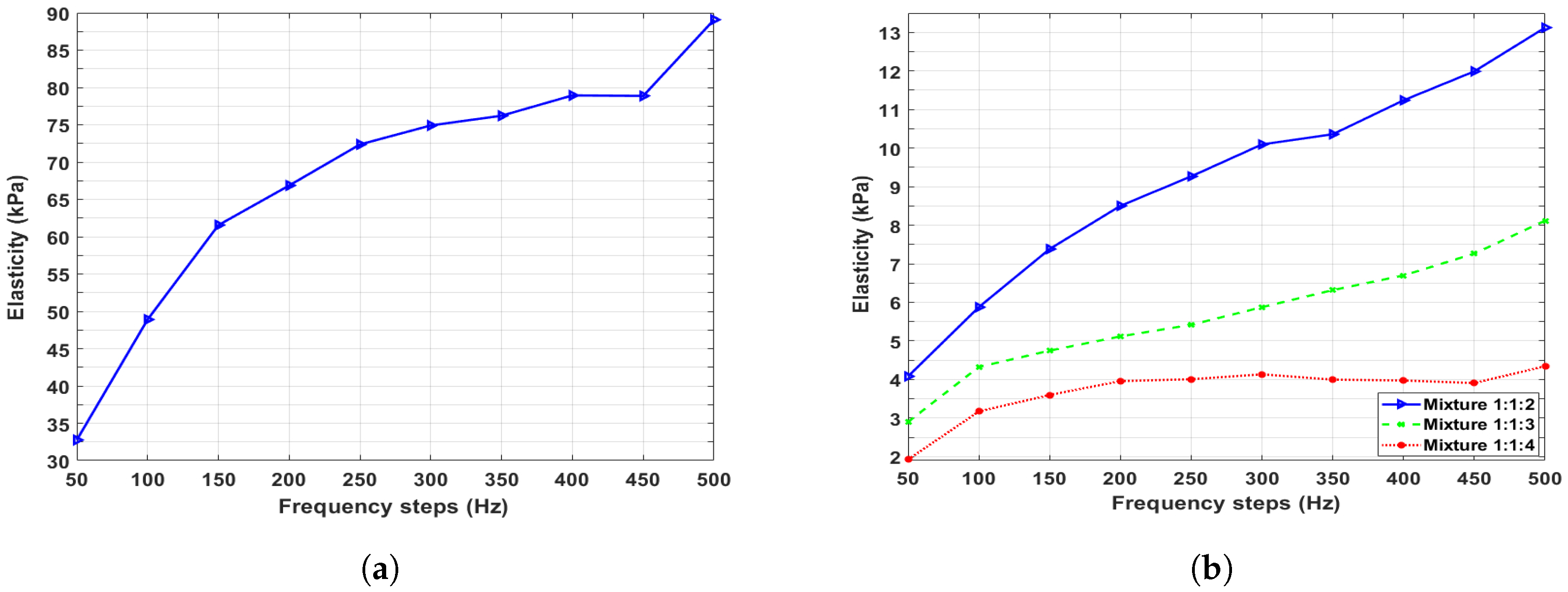
The following measurements were obtained by the smaller pipette depicted in Figure 1a in the second boundary condition, where there is no friction between the sample surface and the tip of the pipette wall. The calculated modulus of elasticity for the four mixtures by Equation (1) are reviewed in Figure 5 versus the frequency steps at which they were excited. The results clearly show the dependency of the modulus of elasticity on the excitation frequency. An elastic modulus of about 36 kPa is determined for the 1:1:0 sample at the 50 Hz while in the same frequency, 4 kPa, 3 kPa and 2 kPa are calculated for the mixtures 1:1:2, 1:1:3 and 1:1:4 respectively. The elastic modulus of the 1:1:0 sample raises to 90 kPa at the excitation frequency 500 Hz. The highest and the lowest values of the calculated elastic modulus belong to the 1:1:0 sample with maximum 90 kPa at 500 Hz and minimum 2 kPa at 50 Hz in the 1:1:4 sample.
5.1.1. Influence of the Excitation Pressure Variations
In the previous studies by Weiss et al. [40] and Zörner et al. [39], the excitation pressure was kept constant over the whole frequency range. These studies showed that the calculated elastic modulus does not depend on the variation of the excitation pressure amplitude. This was examined by using two different samples and pipette radii with two different pressure variation approaches. First, using the smaller pipette, the 1:1:2 mixture excited by the excitation pressure in the frequency range varied in two separate spans, from 2.8 Pa to 12.2 Pa and from 4.2 Pa to 19.2 Pa. Second, the 1:1:3 sample excited in the frequency range by constant 3 Pa pressure and by various pressures from 1 Pa to 12 Pa using the larger pipette. Figure 6, charts (a) and (b), demonstrates amplitudes of the two excitation pressure ranges and the generated displacement. The chart (c) demonstrates the calculated modulus of elasticity by Equation (1) for the 1:1:2 sample in the first approach. The red line in the chart (c) belongs to the calculated modulus of elasticity with the 2.8 Pa to 12.2 Pa range and the blue dotted line denotes the calculated modulus of elasticity with excitation pressure in 4.2 Pa to 19.2 Pa range. It is clear from the results, although the pressure and the generated displacement are different in the two excitation conditions, that the calculated modulus of elasticity remains constant with an acceptable approximation.
For the second approach, the larger pipette with a bigger radius was utilized to excite the 1:1:3 mixture in the experimental setup shown in Figure 1b. The displacement was measured and the modulus of elasticity calculated. The red line of the chart in Figure 7 demonstrates the calculated elastic modulus of the sample by various excitation pressure amplitudes from 1 Pa to 12 Pa and the blue line indicates the calculated modulus of elasticity when the sample is excited with a 3 Pa constant pressure in all the frequency steps. The two lines are completely identical showing that the diversity of the excitation pressure has no effect on the calculated modulus of elasticity using the analytic approximation (1). Comparing Figure 6a and Figure 7 reveals that the calculated modulus of elasticity is independent of the excitation pressure variations using both the pipettes. Therefore, the excitation pressure and the generated displacement amplitude have a linear relation at a fixed frequency.
5.1.2. Influence of the Pipette Tip Compression Force on the Measurements
To investigate the effect of the friction and force of the contact region, the measurement and the numerical simulation were conducted under two different boundary conditions that exhibited different results. The calculated elastic modulus from the measurement by the both pipettes was affected by the force imposed on the silicone surface by the pipette tip wall. All of the previous studies take care of the contact force between pipette and sample cross-section. A transient mount was employed to control the distance of the pipette from the sample surface and a force measurement instrument to control the contact force.
The following are the results of the 1:1:2 mixture which were measured by the smaller pipette in the two defined boundary conditions. Firstly, the pipette touches the sample surface by imposing various grades of force. The pressure and the displacement amplitude is measured when the pipette is connected to the surface applying 0 mN, 10 mN, 50 mN and 100 mN force on the surface. Secondly, the pipette does not touch the silicone surface and is placed at a very small distance. The results of the measurement are demonstrated in Figure 8. The chart (c) shows the calculated modulus of elasticity when the pipette is connected to the surface applying the four different contact forces and when the pipette placed on the surface with a small gap. The graph clearly shows the contact force even in few (mN) could significantly affect the results. In charts (a) and (b), the measured pressure and displacement was illustrated. The measured pressures of the 10 mN, 50 mN and 100 mN are identical in the connected pipette condition, which is reasonable while the generated displacement was different. The lower displacement was generated when the force is higher. This is because the silicone sample surface became more stiff by higher compression force. The displacement amplitude of the pipette with the gap is much lower according to the lower excitation pressure.
The pressure of the 0 mN contact force has a considerable shift compared with the three other contact forces in the connected pipette condition. It may be attributed to inaccuracy in measuring the contact force or the distance between the pipette and the surface in the range of absolute zero. The measured pressure of the 0 mN contact force in the graph (a) is for a condition in which the pipette is not connected to the surface but placed in just a few micrometers distance. Therefore, the pressure of the 0 mN contact force is lower than the other contact forces because of a loss in the pressure amplitude caused by the gap. In the plot, (b) the displacement amplitudes of the 10 mN, 50 mN and 100 mN contact force are gradually increasing by growing the force. While the graph of the 0 mN contact force is not following the previous trend, this clearly shows that the pipette tip wall friction and force have a separate influence on the vibration behaviour of the surface enclosed area by the pipette, which will be discussed in Section 5.2.3.
The results obtained by the bigger pipette is another example that the measured displacement can be affected significantly by the contact force. The pipette in Figure 1b was not fixed to a transient mount and just placed on the sample surface. The pipette’s self-weight acts as a contact force in this condition. Therefore, the calculated modulus of elasticity in plot (c) of Figure 7 and Figure 9 are much higher compared to the results of the smaller pipette depicted in Figure 5. As explained earlier in this section, the pipette weight compresses the surface, so the generated displacements decrease in the denominator of Equation (1) and therefore the calculated modulus of elasticity was boosted.
5.1.3. Vibrational Behavior of the Surface by the Pipette
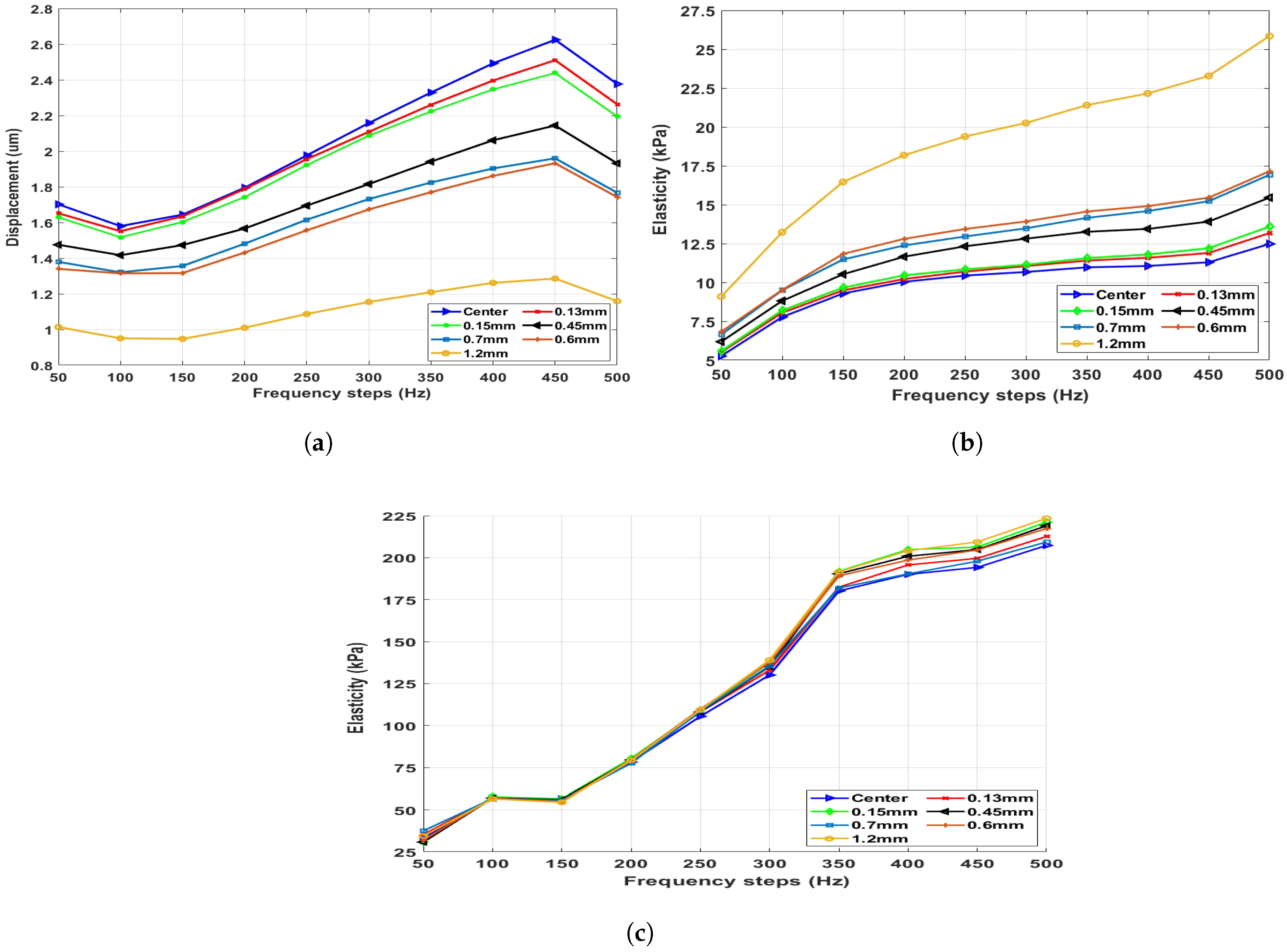
To study the vibrational behavior of the surface surrounded by the pipette, the displacement was measured by various laser spot locations inside the pipette. For understanding the influence of the radius of the surface and the stiffness of the sample in this study, two different pipettes and two different mixtures were used in this section—first, by the smaller pipette with 1.25 mm radius. The pipette touches the sample without applying any force on the surface exactly the same as the connected pipette with 0 mN contact force in the previous subsection. The position of the laser spot changed between seven different locations in the area of a circle with a 2.5 mm diameter within the pipette. The displacement amplitude was measured from the laser spots that were positioned in the center of the pipette and by distances of 0.13 mm, 0.15 mm, 0.45 mm, 0.7 mm, 0.6 mm, 0.7 mm and 1.2 mm from the center, and the modulus of elasticity calculated in the frequency range. The measured displacement by the smaller pipette and the corresponding calculated modulus of elasticity in seven laser spot positions are shown in Figure 9a,b respectively. The blue lines in the graphs denote the displacement amplitude measured from the centre of the pipette and the rest of the lines belong to the other locations inside the pipette with the specified distance from the centre. The legend in the graphs denote the distance of the laser spot locations from the centre of the surface within the pipette. As expected from the behaviour of the model which will be discussed in the Section 5.2.6, the displacement in the centre of this pipette (1.25 mm radius) has the highest value with respect to other locations. The calculated modulus of elasticity from the measured displacement has the lowest value in the centre of the pipette as can be expected.
Second, the position of the laser spot changed between seven different locations in a 3 mm diameter circle on center of the surface surround by the bigger pipette. The diameter of the pipette is 11.5 mm and measurements had been done on the 1:1:0 mixture to examine the effect of mixture stiffness on the results. In this case, the diameter of the surface enclosed by the pipette wall is 11.5 mm, but the laser spot can only move in 3 mm diameter circle in the centre of the enclosed area. Figure 9c shows the calculated elastic modulus of the 1:1:0 mixture in the seven different laser spot locations. The mean value and the standard deviation of the calculated modulus of elasticity in the first and the last frequency step are 34.2 kPa, 2.7 kPa and 214 kPa, 5.5 kPa, respectively.
As is illustrated in the plot (c) of Figure 9, the calculated modulus of elasticity in off-center locations has a lower deviation from the value calculated in the center point, by this bigger pipette with respect to the smaller pipette. Although the laser spot can move in a circle of 2.5 mm diameter in the smaller pipette and in a circle of 3 mm diameter in the bigger pipette which is almost similar, in the first case, the pipette wall restricted the surface in a circle of 3 mm diameter, while the surface is restricted by a diameter of 11.5 mm in the second case. Therefore, a movement in a scale of 100 μm in the centre of a circle with 11.5 mm diameter in the larger pipette produces less deviation with respect to the smaller pipette. On the other hand, the much lower deviation in the mixture 1:1:0 compared to the 1:1:2 mixture in all the excitation frequency steps is also related to its higher stiffness, which causes of lower amplitude of the generated displacement.
5.2. Simulation Results
5.2.1. Connected Pipette
Figure 10 illustrates Young’s modulus of the model and the calculated modulus of elasticity for the 1:1:2 mixture from the measurement in the first boundary approach. In this case, the is restricted in the z-direction but free to move in the x–y axis. In addition, a 100 mN constant force in the z-direction is assigned to the boundary similar to the experimental setup. In the plot (a) of Figure 10, the model Young’s modulus (red line) and the calculated modulus of elasticity by Equation (1) (blue line) is demonstrated. The elastic modulus from the measurement starts from 7.2 kPa and rises to 12.2 kPa while the model Young’s modulus starts from 7.1 kPa and rises to 19.3 kPa. The values of the model Young’s modulus in the simulation fits well with the calculated modulus of elasticity in the first and the second frequency steps, while it starts to go far from the calculated modulus of elasticity in frequencies higher than 100 Hz. As explained earlier at the beginning of Section 4, Young’s modulus of the model after the optimization process can be considered as the reliable estimation of the sample elastic modulus. The discrepancy between the model Young’s modulus and the calculated modulus of elasticity from the measurement comes from the dependency of the elastic modulus on the excitation frequency. Moreover, the agreement between Young’s modulus of the model and the calculated elastic modulus of the sample below 100 Hz shows good capability of the analytical approximation (1), which was developed for calculating static modulus of elasticity also in low frequency dynamic measurement. However, as we are interested in measuring dynamic modulus of elasticity, Equation (1) should be modified by adding a frequency-dependent correction factor to consider the effect of the excitation frequency on the material properties in frequencies higher than 100 Hz. Therefore, a frequency-dependent equation was developed for the connected pipette condition developed by modification in the Aoki et al. [33] analytical approximation (1) as below:
New coefficient is corresponding to the vibration response to a harmonic excitation, which assumed 0.98 for the 1:1:2 sample.
Figure 10 shows Young’s modulus of the model and the elastic modulus calculated with Equation (1) in the plot (a) and with Equation (12) in the plot (b) both from the experimental setup. Figure 10b is exactly identical to the Figure 10a except recalculating the elastic modulus with the new Equation (12). Taking into account the dependency of the elastic modulus of the silicone sample on the excitation frequency by adding the correction factor to Equation (1) causes the results from the experimental setup to be well comparable with Young’s modulus of the model in the simulation, as is demonstrated in Figure 10b.
5.2.2. Pipette with Gap
The Young’s modulus of the model and 1:1:2 mixture’s calculated modulus of elasticity by Equation (1) in the second boundary approach is demonstrated in Figure 11a. The calculated elastic modulus is identical to the graph of the 1:1:2 mixture in Figure 5b, which comes from the measurement. The graphs show the higher Young’s modulus of the model (red line) compared to the calculated modulus of elasticity (blue line). The simulation and measurement results are in the same range but with almost 2 kPa or 3 kPa difference. Since the simulated and the measured displacements are made identical by adjusting the model Young’s modulus, the shift in the tow values is related to the dependency of the material properties on the excitation frequency. Therefore, Equation (1) was modified by a new frequency dependent correction factor to take into account the influence of the excitation frequency for this boundary condition as the following Equation (13). The new coefficient was assumed to be 1.43 for the 1:1:2 sample, which is estimated according to the dependency of the sample displacement profile on the excitation frequency:
Model Young’s modulus and the modulus of elasticity which was calculated from the measurement using Equation (13) demonstrated in Figure 11b. The calculated modulus of elasticity in Figure 11b is exactly the same as Figure 11a except recalculation by Equation (13).
Like in the previous boundary condition, the results of the measurement are fitted with model Young’s modulus by adding a new correction factor to Equation (1). Consequently, the presented acoustic pipette aspiration method has the precise capability to calculate the material frequency-dependent properties (e.g., modulus of elasticity).
5.2.3. The Effect of the Pipette Wall Friction (Gap vs. Connected)
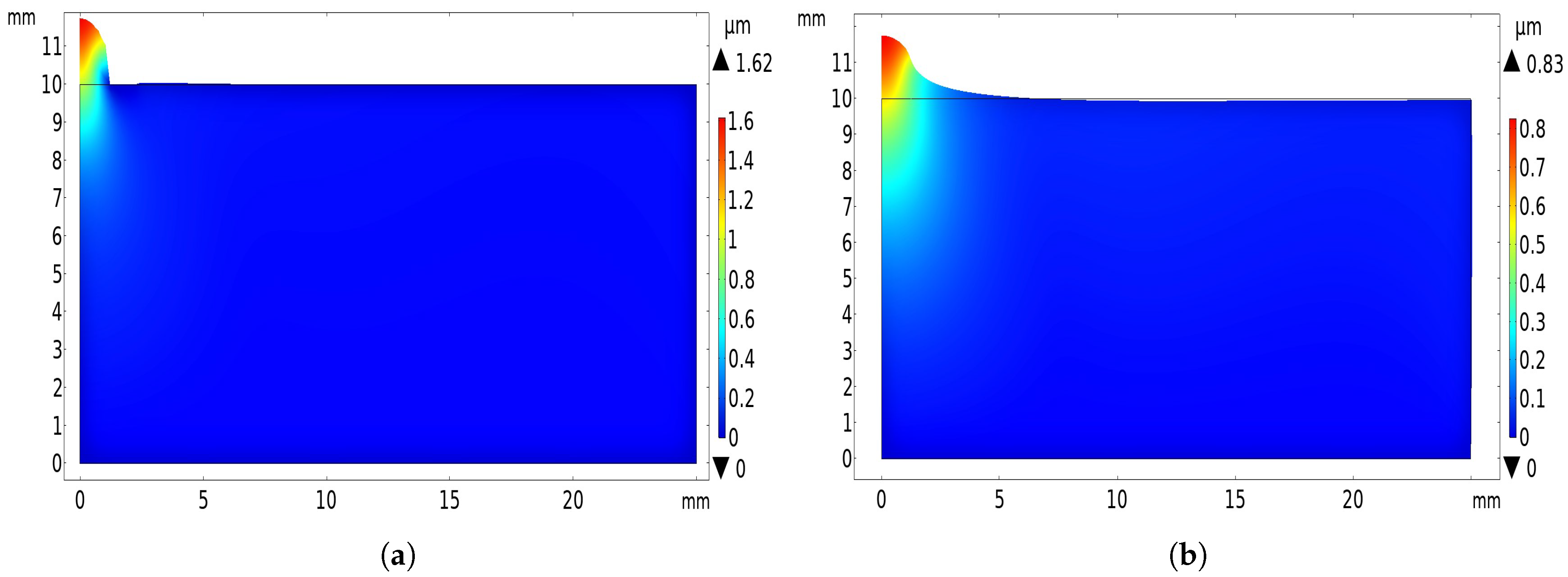
To make the behavior of the model more visible with respect to its response to a dynamic excitation, the surface plot of the displacement amplitude in the z-direction of the first and the last frequency steps in the two boundary conditions are illustrated in Figure 12 and Figure 13. All of the simulation conditions are the same as in Section 5.2.1 and Section 5.2.2. As is shown in Figure 12 the displacement amplitude generated by the 50 Hz excitation pressure is 1.62 μm in the connected pipette while it decreases by almost fifty percent in the pipette with gap boundary condition to 0.83 μm. The displacement amplitude of the 500 Hz excitation pressure is 2.73 μm in the connected pipette condition while it decreases to 1.14 μm by the same ratio in the pipette with gap boundary condition as is demonstrated in Figure 13. The x and left y axes in all the surface plots of this section and the Section 5.2.6, denote the length and height of the model and the right-hand bar is denoting the maximum displacement.
In the connected pipette boundary condition, all of the excitation pressure is transmitted to the silicone surface only within the pipette enclosed area and cannot propagate on the model surface. Therefore, the vibration energy of the excitation pressure is much higher when the pipette is connected to the surface and the resulting displacement is much larger by a factor of two, as demonstrated in Figure 12a and Figure 13a. In the pipette with the gap boundary condition, where the pipette has no friction with the model surface, the excitation energy is distributed also to the outside of the pipette wall. In fact, the excitation pressure is utilized for vibrating a larger area; therefore, the generating displacement in the centre of the pipette is lower than the connected pipette condition. The decreasing ratio of the generated displacement is lower than the decreasing ratio of amplitude of the pressure as it can be understood from the difference between the connected pipette and the pipette with gap plots in Figure 8a,b. This can explain clearly why the calculated elastic modulus is higher in the plot (c) of Figure 8 when the pipette is connected to the surface compared to when the pipette placed on the surface with a gap. Similarly, the model Young’s modulus in the first boundary condition is 7.1 kPa, which is higher than the 6 kPa in the second boundary condition, as is shown in Figure 10a and Figure 11a. The difference comes from the dissimilarity of the pressure and displacement decreasing proportion in the pipette with gap condition. Therefore, Equation (13) was developed to take into account this nonlinear relation in the calculation.
5.2.4. Damping Analysis
The effect of the damping factor on the simulated results of the two boundary conditions was investigated by assigning various damping factors to the model and comparing the displacement predictions. 0.13 assigned to the damping ratio 1 () in the first frequency step = 50 Hz and 0.25 to damping ratio 2 () in the last frequency step = 500 Hz. Then, the first damping ratio () varied from 0.1 to 0.4 and the second () varied from 0.225 to 0.400. Figure 14 shows the z-component of the displacement amplitude with respect to the variation of the damping ratios in the two boundary conditions.
High dependency on the damping factor is visible from the graphs in both boundary conditions, especially in frequencies higher than 200 Hz. While, as it should be, this dependency is much lower in the low frequencies, especially in the connected pipette condition. The displacement predictions by damping ratios 0.13 for 50 Hz and 0.25 for 500 Hz were well fit with the measured displacement, which is specified with the green dotted line in figure. This shows that the two damping ratios extracted from the previous studies [54,55] are precise.
5.2.5. Poisson’s Ratio Analysis
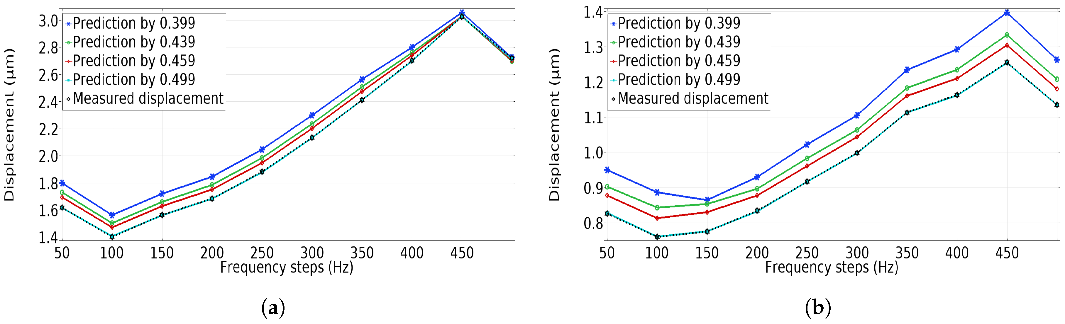
To investigate the effect of the Poisson’s ratio on prediction of the model displacement in the two boundary conditions, an analysis in the range of 0.399 to 0.499 was performed in the two boundary conditions. The range 0.399 to 0.499 is extracted from the previous studies [45,54,55] for the mixture 1:1:2, which the model is based on. The range was chosen to cover the Poisson’s ratios determined by tensile test [45] and by dynamic measurement setup [54,55] from 0.45 to 0.499. The model predictions of the displacement z-component by the four different Poisson’s ratios are demonstrated in Figure 15.
High dependency on the Poisson’s ratio is visible from the plots in both boundary conditions, especially in the pipette with gap condition. Apart from the previous studies [54,55] in which the Poisson’s ratio of a harmonically excited sample determined close to 0.5, the measured displacement which is denoted with the black dotted line in the graphs fits better with the predictions of displacement using Poisson’s ratio 0.499. Therefore, we use Poisson’s ratio 0.499 for the model in the simulation. Both graphs show that the Poisson’s ratio can be assumed constant in the frequency range as is assumed in the previous studies [54,55].
5.2.6. Influence of the Pipette Radius
More than the pipette wall thickness, specimen thickness and specimen radius, the radius of the pipette can affect the results. In Aoki et al. [33], the static measurement setup assumed that a change in the pipette radius causes a change in the displacement amplitude with an equal ratio. In other words, increasing or decreasing the pipette radius will cause an increase or decrease in the displacement amplitude with an equal factor. While the measured displacement from our dynamic experimental setup is revealed to have high dependency on the radius of the pipette with respect to the excitation frequency, the frequency-dependent relation violates the Aoki et al. [33] assumption after a certain radius size and especially in frequencies higher 100 Hz. This behaviour is seen also in the simulation results as follows: Figure 16 shows the z-component of the simulated displacement amplitude in the center of the pipette versus the frequency range by six different pipette radii. The displacement is almost constant over the frequency range using a very small radius, 0.25 mm, while, in both boundary conditions, the displacement amplitude is a function of the excitation frequency for radii larger than 0.25 mm. The displacement grows with increasing frequency in radii lower than 1.25 mm, but this trend will inverse if the pipette radius exceeds 1.25 mm. For the higher radii 3.25 mm, 4.25 mm and 5.25 mm, the displacement falls with moving forward in the frequency steps. Consequently, the displacement has a nonlinear relation with the pipette radius after a certain radius, so the radius could not exceed a certain limit in a dynamic measurement.
It can be supposed from a static measurement that, if the pipette encloses the surface with a larger radius, the generated displacement should have a higher amplitude because of the larger space for vibration, while, with harmonic excitation, the larger space made the surface able to resonate. This can be concluded from Figure 16 where the displacement amplitude (in the centre of the pipette) falls more in the higher radii. In both boundary conditions, a high radius causes resonance on the surface after 100 Hz excitation frequency. Therefore, the displacement amplitude on the centre of the pipette is decreased significantly. Similar to the Aoki et al. [33] static measurement, the increasing ratios of the displacement amplitude and the radius are equal in 50 Hz excitation frequency.
To explain better, the resonance behaviour of the model as a function of the pipette radius, the surface plot of the displacement amplitude generated by 500 Hz excitation frequency for two different radii 1.25 mm and 5.25 mm are illustrated in Figure 17 and Figure 18. The displacement z-component of the connected pipette boundary condition is shown in Figure 17 and, of the pipette with gap boundary condition, shown in Figure 18. All the simulation conditions are exactly the same as Section 5.2.1 and Section 5.2.2 except a phase () assigned to the fluctuating force to make the behaviour of the model in the plots more understandable. The scale factor of the plots is 1000. As are shown in Figure 17a and Figure 18a, the high radius of the pipette made the surface resonant; as a result, the maximum displacement amplitude falls and moves from the centre of the pipette. Figure 17b shows that the maximum displacement amplitude of the 1.25 mm surface radius 2.75 μm in the centre of the pipette. While, because of the resonance induced due to the larger radius 5.25 mm, the maximum displacement falls from 2.75 μm to 1.24 μm and moves from the centre, as is depicted in Figure 17a. Moreover, the displacement amplitude in the centre of the pipette declines from 2.75 μm in radius 1.25 mm to almost 0.5 μm in the radius 5.25 mm.
The same behavior in the pipette with gap boundary condition is visible from Figure 18. However, the resonance effect is weaker because the model surface is not restricted by the pipette wall in this boundary condition. As a result, the maximum displacement amplitude is lower than the connect pipette condition. Figure 18 demonstrates surface plots of the displacement amplitude of the radius 5.25 mm and the radius 1.25 mm in the pipette with gap boundary condition.
Similar to the connected pipette boundary condition, the maximum displacement decreases from 1.14 μm in radius 1.25 mm to 0.56 μm in radius 5.25 mm, which is shown in Figure 18. The decrements ratio is almost 2, a little less than the connected pipette condition, which is almost 2.2. Moreover, comparing the plot (a) of Figure 17 and Figure 18 exhibits the maximum displacement position moving to a farther point from the centre in the pipette with a gap with respect to the connected pipette boundary condition.
6. Discussion
6.1. Capability of the Aoki et al. Equation (1) for a Dynamic Experimental Setup
To investigate the capability of Equation (1) for calculation of the artificial and real vocal folds tissue elastic modulus, we performed the measurement in a wider frequency range from 50 Hz to 500 Hz compared to the previous studies. The results of Section 5.2.1 and Section 5.2.2 revealed a strong dependency of the model Young’s modulus on the excitation frequency. Therefore, as is demonstrated in Figure 10a, the equation can be an accurate approximation of the silicone sample modulus of elasticity only in frequencies lower than 100 Hz, while, in the higher frequencies, the equation does not have the proper functionality and leads to error. Moreover, since, in a dynamic measurement, many of the material properties are a function of the excitation frequency as are explained in Section 5, the impact of the equation items on the calculation may change by the excitation frequency. On the other hand, the effect of the pipette wall contact force and friction and the radius of the pipette which is also related to the excitation frequency should be considered in an analytical approximation for estimating the modulus of elasticity. Therefore, the Equation (1) cannot be used for the frequency range of human speech. We modified the equation by adding a new correction factor considering the effect of the excitation pressure frequency for both the boundary conditions as the Equations (12) and (13).
6.2. Capability of the Correction Factors in Equations (12) and (13) to Cover a Broad Range of Cases
The two correction coefficients in Equations (12) and (13) are developed specifically for the 1:1:2 mixture and under certain pipette-surface contact boundary conditions. Therefore, the coefficients could be used just for the produced 1:1:2 mixture and with equal contact compression force and gap size in which we did the measurements. In future work, the two correction coefficients should be examined for the other three mixtures to investigate the feasibility of using them for a broad range of cases. This could be a further step in developing the pipette aspiration technique in the future. However, developing two unique coefficients for all the four mixture is so challenging. This is due to the high dependency of the two terms of the Equation (1), the generated displacement and excitation pressure, on the boundary condition. As it is indicated in Figure 8, the results depend very strongly on the exact value of the compression force and on the gap size. Therefore, in order to make it possible to develop two unique correction coefficients, the boundary conditions should be exactly equal for all the four mixtures. While uncertainty in measuring equally the pipette-surface contact boundary condition in all the four mixtures is inevitable in the presented experimental setup, the uncertainty comes from the accuracy of measuring the boundary condition. The accuracy should be in the range of tens of (μm) and hundreds of (μN) for this purpose.
6.3. Effect of the Compression Force on the Measurement
The previous studies [33,39,40] show that the contact force between the pipette tip border and the sample surface has an impact on the measurement, while the effect of the pipette tip wall compression force and friction on the sample surface behaviour has not been studied yet. In this present study, the measurement and the simulation were done in the two boundary approaches, connected pipette and pipette with gap conditions. The results revealed that the friction or the tangential displacement constraint and the force at the sample-pipette contact region can separately affect the present linear analysis significantly. Comparing the graphs in Figure 8 clearly shows that the measured pressures in the 10 mN, 50 mN and 100 mN are identical while the generated displacements are lower when the pipette applies more compression force on the silicone surface. This is because, when the surface is under compression, it became harder; therefore, with identical excitation pressure, the lower displacement is generated when the force is higher.
On the other hand, the problem of using a small gap to prevent the pipette tip wall compression force on the surface is that the excitation pressure lessens and therefore the generated displacement amplitude declines. The generated displacement and the excitation pressure have a nonlinear relation when the pipette is placed on the surface with gap. By comparing the model Young’s modulus, which is considered as the true value of the sample modulus of elasticity, with the calculated modulus of elasticity in Figure 11, it can be concluded that the calculated modulus of elasticity declines unrealistically in the pipette with gap boundary conditions. We add a new correction factor to the Equation (1) to take into account the nonlinear relation in the calculation to make a suitable analytic approximation for pipette with gap boundary condition as the Equation (13) for the present study.
Using a gap can cancel the impact of the pipette tip wall compression force and friction, which are the major causes of uncertainty, but, if a connection between the pipette and the surface is unpreventable, the contact compression force should be restricted to absolutely zero. As depicted by the connected pipette index in Figure 8, the compression force even in a range of tens of (mN) can interfere in the measurement. Furthermore, the force scale is based on the mixture stiffness; in the softer mixtures, the force in hundreds of (μN) range can act on the behaviour of the surface. If the pipette tip compression force is unavoidable, the Aoki et al. equation will need further modification by adding a term considering the influence of the force.
6.4. Sensitivity of Results to the Pipette-Surface Boundary Condition
As indicated in Figure 8, the excitation pressure and the generated displacement on the sample surface is highly sensitive to the boundary condition. Since the excitation pressure and the generated displacement are the two fundamental terms of Equation (1), the calculated elastic modulus also has a high dependency on the boundary condition. The sensitivity comes from the strong dependency of the generated displacement amplitude on the sample surface to the contact compression force on one side and to the excitation pressure amplitude on the other side. As discussed earlier, the compression force makes the sample surface harder and causes the measured displacement decline by applying higher contact pressures. Furthermore, when the size of the gap gets larger, the excitation pressure on the surface falls and the generated displacement amplitude also declines in this case. Therefore, controlling the contact compression force or the gap size is necessary for the accuracy of this presented method. The pipette with gap boundary condition is our preferred method because the compression force does not exist to affect the hardness of the surface and controlling of the gap size is much easier than the compression force. By monitoring the excitation pressure amplitude from the microphone input by the Labview automation program continuously, the gap size could be controlled quite well. An excitation pressure value could be measured for the desired gap size and be defined as an index for the acceptable gap size in the automation program. The pressure is expected to be almost constant in the desired gap size while it might increase or decrease instantly if the pipette touched the surface or the gap size became large. During the measurement, if the excitation pressure goes lower or higher than the threshold index, the automation program shows that the gap size in the measurement is not appropriate and results are not acceptable. Using the connected pipette is not suggested by this study because this method is more sensitive to the exact boundary condition than the pipette with gap method. The compression force has a significant effect on the correctness of the calculated elastic modulus of the sample surface, especially at higher contact pressures. Moreover, controlling the compression pressure and correcting the errors caused by the pressure is much more complicated compared to the pipette with a gap boundary condition method.
6.5. Effect of the Radius of the Pipette on the Measurement
In the Aoki et al. [33] static measurement setup, a variation in the employed pipette radius is assumed to generate a displacement with equal ratio. In other words, the displacement amplitude was assumed to have a linear relation with the radius of the pipette. While the measured displacement by the two different pipette radii revealed a nonlinear relation between the measured displacement and radius of the pipette, the relation is linear only for a very small radius in a few hundreds of (μm) range. The high radius of the pipette causes resonance on the silicone surface surrounded by the pipette wall so the displacement on the centre of the pipette falls significantly. Therefore, due to the resonance behaviour of the sample surface, the pipette radius could not exceed a certain limit in dynamic measurement.
High spatial resolution and less error in the measurement is attainable with reducing the pipette radius as low as possible. If pipette radius should be larger than a certain limit for a special application, the Aoki et al. [33] equation will need further modification by adding a new term considering the dependency of the displacement profile on the radius of the pipette, which is a function of frequency.
6.6. Effect of the Damping Factor and the Poisson’s Ratio
In previous studies [39], a constant damping ratio in the frequency range was assigned to a model, while, as discussed earlier in the Section 5.2.4 and Section 5.2.5, the results of the simulation show that the vibrational behaviour of the silicone surface under the pipette with regard to the damping factor and Poisson’s ratio is frequency dependent. This dependency exhibits itself more according to the sample consistency and the excitation frequency. For the softer mixtures and in the higher frequencies, the influence of the damping factor and Poisson’s ratio in the model computations is higher. As is demonstrated in Figure 14 and Figure 15, the simulated displacement has the best fit to the measured displacement by taking the damping factors 0.13 for 50 Hz and 0.25 for 500 Hz and the Poisson’s ratio close to 0.5.
6.7. Effect of the Excitation Pressure Amplitude
The excitation pressure was kept constant over the frequency range in the previous studies [39,40]. While the present study results demonstrated in Figure 6c and Figure 7 show that the calculated modulus of elasticity is independent of the excitation pressure amplitude variations, it can be concluded that the excitation pressure and the generated displacement amplitude have a linear relation at a fixed frequency and the pipette radius diversity cannot affect the linear relationship.
6.8. Linear Elastic Behavior of the Model
Since we are in the first phase of this project, a simplified model of the experimental setup with a linear elastic material formulation was used in this present study, while using hyperelastic models for describing the nonlinear elastic behaviour of the model could be future work in this project. Furthermore, the generated displacement in the (μm) range is really small compared to the dimension of the samples and vocal fold tissue in the (mm) range. Therefore, we can only measure the linear part of the elastic modulus with this measurement method. Nonlinear characteristics would have to be measured with higher excitation pressure and higher generated displacement. The main goal in this phase is to develop the pipette aspiration method by using an acoustic pressure excitation and examine its functionality for characterization of the frequency-dependent material properties of the silicone rubber mixtures and real vocal fold tissue.
7. Conclusions
We presented a measurement method to determine the frequency-dependent elastic modulus of silicone rubber mixtures that are used for synthetic vocal folds models. Therewith, a silicone specimen was placed under a pipette, which is used to channel the acoustic pressure generated by a tiny loudspeaker. Two different conditions were defined for pipette sample cross-section boundaries. First, the pipette was pressed against the sample surface by applying several contact forces in the range of 0 to 100 mN. Second, the pipette was placed on the surface with a very small gap. The calculated elastic modulus for the four silicone mixtures shows an increase over the frequency range and was in the range of 2.1 kPa to 90 kPa for the smaller pipette. To verify the functionality of the presented measurement setup for characterization of the dynamic material properties of the silicone rubber and real tissue, numerical simulation by a finite element method using a simplified model of the experimental setup was performed under the two boundary conditions that exhibit a significant difference in the results. The influence of the harmonic excitation on the model Young’s modulus, Poisson’s ratio, the damping factor and resonance behavior of the surface was discovered by the simulation. Young’s modulus and damping factor of the model increase over the excitation frequency range. The results show that the damping factor of the model is frequency-dependent and 0.13 for 50 Hz and 0.25 for 500 Hz and cannot be assumed constant over the human speech frequency range, while the Poisson’s ratio was close to 0.5 and can be assumed constant in the frequency range, as shown in the previous studies [39,40,54,55].
Since the lack of the equation dependency on the excitation frequency, resonance effect and the absence of considering the impact of the pipette tip wall force and friction was revealed in the measurement and simulation results, it can be concluded that the Aoki et al. [33] analytic approximation cannot be used for a dynamic measurement in the range of human speech frequency [38]. We modified the Aoki et al. Equation (1) by adding a frequency-dependent factor to calculate silicone rubber elastic modulus at the two boundary conditions. Recalculating the samples modulus of elasticity with the new analytical approximations made the results of measurement fit well with model Young’s modulus in both boundary conditions. Consequently, the presented acoustic pipette aspiration method has the precise capability to calculate the material frequency-dependent properties (e.g., modulus of elasticity).
Using a gap can cancel the impact of the pipette tip compression force and friction, which are the major causes of uncertainty, but, if a connection between the pipette and the surface is unpreventable, the contact compression force should be restricted to absolutely zero. Moreover, since the frequency-dependent relationship between the displacement profile and the pipette radius was seen because of the surface resonance, the radius could not exceed a certain limit in a dynamic measurement. Furthermore, the measurement results revealed (see e.g., Section 5.1.1) that the displacement profile has a linear relation with the excitation pressure at a fixed frequency when the pipette is connected to surface by a fixed compression force and the pipette radius diversity cannot affect this linear relationship in this present method.
The present results were in good agreement with the corresponding analytical results obtained by Weiss et al. [40] and Zörner et al. [39]. Extreme miniaturization and simplicity of the presented measurement setup are the key benefits of the developed method in comparison to the previous studies using a pistonphone. Further work is underway toward investigations on excised tissue and the comparison of real and synthetic vocal folds material characterization. Since the displacement was measured by a laser vibrometer, the poor reflectivity and roughness of real tissue might be a challenging issue.
Author Contributions
Conceptualization, A.S. and M.M.; methodology, A.S. and M.M.; software, M.M.; validation, M.M. and A.S.; formal analysis, M.M. and A.S.; investigation, M.M.; resources, M.M. and A.S.; writing—original draft preparation, M.M.; writing—review and editing, R.L., M.S., A.S. and M.M.; visualization, M.M.; supervision, A.S.; project administration, A.S.; funding acquisition, A.S.
Funding
This research was funded by the Austrian Science Fund Grant No. I 3806-B28 and by the German research foundation (DFG) No. DO1247/9-1.
Acknowledgments
We acknowledge the Open Access Funding by the Austrian Science Fund (FWF) and German research foundation (DFG).
Conflicts of Interest
The authors declare no conflict of interest.
References
- Heris, H.K.; Miri, A.K.; Tripathy, U.; Barthelat, F.; Mongeau, L. Indentation of poroviscoelastic vocal fold tissue using an atomic force microscope. J. Mech. Behav. Biomed. Mater. 2013, 28, 383–392. [Google Scholar] [CrossRef] [PubMed] [Green Version]
- Miri, A.K. Mechanical Characterization of Vocal Fold Tissue: A Review Study. J. Voice 2014, 28, 657–667. [Google Scholar] [CrossRef] [PubMed]
- Childers, D.G.; Wong, C.F. Measuring and modeling vocal source-tract interaction. IEEE Trans. Biomed. Eng. 1994, 41, 663–671. [Google Scholar] [CrossRef] [PubMed]
- Yan, Y.; Chen, X.; Bless, D. Automatic tracing of vocal-fold motion from high-speed digital images. IEEE Trans. Biomed. Eng. 2006, 53, 1394–1400. [Google Scholar] [CrossRef] [PubMed]
- Tao, C.; Zhang, Y.; Jiang, J.J. Extracting physiologically relevant parameters of vocal folds from high-speed video image series. IEEE Trans. Biomed. Eng. 2007, 54, 794–801. [Google Scholar] [PubMed]
- Lohscheller, J.; Eysholdt, U.; Toy, H.; Döllinger, M. Phonovibrography: Mapping high-speed movies of vocal fold vibrations into 2D diagrams for visualizing and analyzing the underlying laryngeal dynamics. IEEE Trans. Biomed. Eng. 2008, 27, 300–309. [Google Scholar] [CrossRef] [PubMed]
- Qin, X.; Wang, S.; Wan, M. Improving reliability and accuracy of vibration parameters of vocal folds based on high-speed video and electroglottography. IEEE Trans. Biomed. Eng. 2009, 56, 1744–1754. [Google Scholar]
- Goodyer, E.; Jiang, J.J.; Devine, E.; Sutor, A.; Rupitsch, S.; Zörner, S.; Stingl, M.; Schmidt, B. Devices and methods on analysis of bio-mechanical properties of laryngeal tissue and substitute materials. Curr. Bio-Inform. 2011, 6, 344–361. [Google Scholar] [CrossRef]
- Dion, G.R.; Jeswani, S.; Roof, S.; Fritz, M.; Coelho, P.G.; Sobieraj, M.; Amin, M.R.; Branski, R.C. Functional assessment of the ex vivo vocal folds through biomechanical testing: A review. Mater. Sci. Eng. C Mater. Biol. Appl. 2016, 64, 444–453. [Google Scholar] [CrossRef] [Green Version]
- Cook, D.D.; Nauman, E.; Mongeau, L. Ranking vocal fold model parameters by their influence on modal frequencies. J. Acoust. Soc. Am. 2009, 126, 2002–2010. [Google Scholar] [CrossRef]
- Alipour-Haghighi, F.; Titze, I.R. Elastic models of vocal fold tissues. J. Acoust. Soc. Am. 1991, 90, 1326–1331. [Google Scholar] [CrossRef] [PubMed]
- Kelleher, J.E.; Zhang, K.; Siegmund, T.; Chan, R.W. Spatially varying properties of the vocal ligament contribute to its eigenfrequency response. J. Mech. Behav. Biomed. Mater. 2010, 3, 600–609. [Google Scholar] [CrossRef] [PubMed] [Green Version]
- Döllinger, M.; Berry, D.A.; Hüttner, B.; Bohr, C. Assessment of local vocal fold deformation characteristics in an in vitro static tensile test. J. Acoust. Soc. Am. 2011, 130, 977–985. [Google Scholar] [CrossRef] [PubMed]
- Kelleher, J.E.; Siegmund, T.; Chan, R.W.; Henslee, E.A. Optical measurements of vocal fold tensile properties implications for phonatory mechanics. J. Bio-Mech. 2011, 44, 1729–1734. [Google Scholar] [CrossRef] [PubMed]
- Kataoka, N.; Ohashi, T.; Matsumoto, T.; Aoki, T.; Sato, M. Application of the pipette aspiration technique to the measurement of local elastic moduli of cholesterol-fed rabbit aortas. Theor. Appl. Mech. 1994, 43, 233–238. [Google Scholar]
- Story, B.H.; Titze, I.R. Voice simulation with a body-cover model of the vocal folds. J. Acoust. Soc. Am. 1995, 97, 1249–1260. [Google Scholar] [CrossRef] [PubMed]
- Döllinger, M.; Hoppe, U.; Hettlich, F.; Lohscheller, J.; Schuberth, S.; Eysholdt, U. Vibration parameter extraction from endoscopic image series of the vocal folds. IEEE Trans. Biomed. Eng. 2002, 49, 773–781. [Google Scholar] [CrossRef] [PubMed]
- Neubauer, J.; Zhang, Z.; Miraghaie, R.; Berry, D.A. Coherent structures of the near field flow in a self-oscillating physical model of the vocal folds. J. Acoust. Soc. Am. 2007, 121, 1102–1118. [Google Scholar] [CrossRef] [PubMed]
- Chan, R.W.; Rodriguez, M.L. A simple-shear rheometer for linear viscoelastic characterization of vocal fold tissues at phonatory frequencies. J. Acoust. Soc. Am. 2008, 124, 1207–1219. [Google Scholar] [CrossRef]
- Lamprecht, R.; Maghzinajafabadi, M.; Semmler, M.; Sutor, A. Imaging the vocal folds: A feasibility study on strain imaging and elastography of porcine vocal folds. Appl. Sci. 2019, 9, 2729. [Google Scholar] [CrossRef]
- Becker, S.; Kniesburges, S.; Müller, S.; Delgado, A.; Link, G.; Kaltenbacher, M.; Döllinger, M. Flow-structure-acoustic interaction in a human voice model. J. Acoust. Soc. Am. 2009, 125, 1351–1361. [Google Scholar] [CrossRef] [PubMed]
- Zhang, Z.; Neubauer, J.; Berry, D.A. Influence of vocal fold stiffness and acoustic loading on flow-induced vibration of a single layer vocal fold model. J. Sound Vib. 2009, 322, 299–313. [Google Scholar] [CrossRef] [PubMed]
- Zhang, Z. Characteristics of phonation on set in a two-layer vocal fold model. J. Acoust. Soc. Am. 2009, 125, 1091–1102. [Google Scholar] [CrossRef] [PubMed]
- Owaki, S.; Kataoka, H.; Shimizu, T. Relationship between transglottal pressure and fundamental frequency of phonation-study using a rubber model. J. Voice 2010, 24, 127–132. [Google Scholar] [CrossRef] [PubMed]
- Chan, R.W.; Titze, I.R. Viscoelastic shear properties of human vocal fold mucosa: Measurement methodology and empirical results. J. Acoust. Soc. Am. 1999, 106, 2008–2021. [Google Scholar] [CrossRef] [PubMed]
- Rand, R.P.; Burton, A.C. Mechanical properties of the red cell membrane, I. membrane stiffness and intra-cellular pressure. Biophys. J. 1964, 4, 115–135. [Google Scholar] [CrossRef]
- Cook, T.; Alexander, H.; Cohen, M.L. Experimental method for determining the two-dimensional mechanical properties of living human skin. Med. Biol. Eng. Comput. 1977, 15, 381–390. [Google Scholar] [CrossRef]
- Sato, M.; Levesque, M.J.; Nerem, R.M. An application of the micropipette technique to the measurement of the mechanical properties of cultured bovine aortic endothelial cells. J. Bio-Mech. Eng. 1987, 109, 27–34. [Google Scholar] [CrossRef]
- Theret, D.P.; Levesque, M.J.; Sato, M.; Nerem, R.M.; Wheeler, L.T. The application of a homogeneous half-space model in the analysis of endothelial cell micropipette measurements. J. Bio-Mech. Eng. 1988, 110, 190–199. [Google Scholar] [CrossRef]
- Evans, E.A. New membrane concept applied to the analysis of fluid shear- and micropipette-deformed red blood cells. Biophys. J. 1973, 13, 941–954. [Google Scholar] [CrossRef]
- Matsumoto, T.; Abe, H.; Ohashi, T.; Kato, Y.; Sato, M. Local elastic modulus of atherosclerotic lesions of rabbit thoracic aortas measured by pipette aspiration method. Physiol. Meas. 2002, 23, 635–648. [Google Scholar] [CrossRef] [PubMed]
- Ohashi, T.; Abe, H.; Matsumoto, T.; Sato, M. Pipette aspiration technique for the measurement of nonline and anisotropic mechanical properties of blood vessel walls under biaxial stretch. J. Biomech. 2004, 38, 2248–2256. [Google Scholar] [CrossRef] [PubMed]
- Aoki, T.; Ohashi, T.; Matsumoto, T.; Sato, M. The pipette aspiration applied to the local stiffness measurement of soft tissues. Ann. Biomed. Eng. 1997, 25, 581–587. [Google Scholar] [CrossRef] [PubMed]
- Long, J.L.; Neubauer, J.; Zhang, Z.; Zuk, P.; Berke, G.S.; Chhetri, D.K. Functional testing of a tissue-engineered vocal fold cover replacement. Otolaryngol. Head Neck Surg. 2010, 142, 438–440. [Google Scholar] [CrossRef] [PubMed]
- Miri, A.K.; Heris, H.K.; Mongeau, L.; Javid, F. Nanoscale viscoelasticity of extracellular matrix proteins in soft tissues: A multiscale approach. J. Mech. Behav. Biomed. Mater. 2014, 30, 196–204. [Google Scholar] [CrossRef]
- Ohsumi, A.; Nakano, N. Identification of physical parameters of a flexible structure from noisy measurement data. IEEE Trans. Instrum. Meas. 2002, 51, 923–929. [Google Scholar] [CrossRef]
- Lu, M.H.; Yu, W.; Huang, Q.H.; Huang, Y.P.; Zheng, Y.P. A handheld indentation system for the assessment of mechanical properties of soft tissues in vivo. IEEE Trans. Instrum. Meas. 2009, 58, 3079–3085. [Google Scholar]
- Hollien, H.; Dew, D.; Philips, P. Phonational frequency ranges of adults. J. Speech Lang. Hear. Res. 1971, 14, 755–760. [Google Scholar] [CrossRef]
- Zörner, S.; Kaltenbacher, M.; Lerch, R.; Sutor, A.; Döllinger, M. Measurement of the elastic modulus of soft tissues. J. Biomech. 2010, 43, 1540–1545. [Google Scholar] [CrossRef]
- Weiss, S.; Sutor, A.; Ilg, J.; Rupitsch, S.J.; Lerch, R. Measurement and analysis of the material properties and oscillation characteristics of synthetic vocal folds. Acta Acust. United Acust. 2016, 102, 214–229. [Google Scholar] [CrossRef]
- Weiss, S.; Thomson, S.L.; Sutor, A.; Rupitsch, S.J.; Lerch, R. Influence of pipette geometry on the displacement profile of isotropic materials used for vocal fold modeling. Int. Conf. Biomed. Electron. Devices Biodevices 2013, 102, 108–113. [Google Scholar]
- Weiss, S.; Thomson, S.L.; Lerch, R.; Döllinger, M.; Sutor, A. Pipette aspiration applied to the characterization of nonhomogeneous, transversely-isotropic materials used for vocal fold modeling. J. Mech. Behav. Biomed. Mater. 2013, 17, 137–151. [Google Scholar] [CrossRef]
- Goodyer, E.; Müller, F.; Licht, K.; Hess, M. In vivo measurement of the shear modulus of the human vocal fold: Interim results from eight patients. Eur. Arch. Oto-Rhino-Laryngol. 2007, 264, 631–635. [Google Scholar] [CrossRef]
- Rupitsch, S.J.; Wolf, F.; Sutor, A.; Lerch, R. Estimation of material parameters for piezoelectric actuators using electrical and mechanical quantities. In Proceedings of the 2009 IEEE Ultrasonics Symposium, Rome, Italy, 20–23 September 2009; pp. 414–417. [Google Scholar]
- Drechsel, J.S. Characterization of Synthetic, Self-Oscillating Vocal Fold Models. Master’s Thesis, Brigham Young University, Provo, UT, USA, 2007. [Google Scholar]
- Drain, L.E. The Laser Doppler Techniques, 1st ed.; Wiley-Interscience: Chichester, UK, 1980. [Google Scholar]
- Link, G.; Kaltenbacher, M.; Döllinger, M. A 2d finite-element scheme for fluid solid acoustic interactions and its application to human phonation. Comput. Methods Appl. Mech. Eng. 2009, 198, 3321–3334. [Google Scholar] [CrossRef]
- Chan, R. Measurements of vocal fold tissue viscoelasticity: Approaching the male phonatory frequency range. J. Acoust. Soc. Am. 2004, 115, 3161–3170. [Google Scholar] [CrossRef] [PubMed]
- Chan, R.W. Estimation of viscoelastic shear properties of vocal-fold tissues based on time temperature superposition. J. Acoust. Soc. Am. 2001, 110, 1548–1561. [Google Scholar] [CrossRef] [PubMed]
- Willis, R.L.; Shane, T.S.; Berthelot, H.Y.; Madigosky, W.M. An experimental-numerical technique for evaluating the bulk and shear dynamic moduli of viscoelastic materials. J. Acoust. Soc. Am. 1997, 102, 3549–3555. [Google Scholar] [CrossRef]
- Chan, R.W.; Fu, M.; Tirunagari, N. Elasticity of the human false vocal fold. Ann. Otol. Rhinol. Laryngol. 2006, 115, 370–381. [Google Scholar] [CrossRef]
- Willis, R.L.; Wu, L.; Berthelot, H.Y. Determination of the complex Young and shear dynamic moduli of viscoelastic materials. J. Acoust. Soc. Am. 2001, 109, 611–621. [Google Scholar] [CrossRef]
- Wojtowicki, J.L.; Jaouen, L.; Panneton, R. New approach for the measurement of damping properties of materials using the Oberst beam. Rev. Sci. Instrum. 2004, 75, 2569–2574. [Google Scholar] [CrossRef] [Green Version]
- Rupitsch, S.J.; Ilg, J.; Sutor, A.; Lerch, R.; Döllinger, M. Simulation based estimation of dynamic mechanical properties for viscoelastic materials used for vocal fold models. J. Sound Vib. 2011, 330, 4447–4459. [Google Scholar] [CrossRef]
- Ilg, J.; Rupitsch, S.J.; Sutor, A.; Lerch, R. Determination of dynamic material properties of silicone rubber using one-point measurements and finite element simulations. IEEE Trans. Instrum. Meas. 2012, 61, 3031–3038. [Google Scholar] [CrossRef]
- Kaltenbacher, M. Numerical Simulation of Mechatronic Sensors and Actuators, 3rd ed.; Springer: Berlin, Germany, 2015; pp. 93–114. [Google Scholar]
- Krasnosel’skii, M.A.; Pokrovskii, A. Systems with Hysteresis, 1st ed.; Springer: Berlin, Germany, 1989. [Google Scholar]
- Mayergoyz, I.D. Mathematical Models of Hysteresis, 1st ed.; Springer: New York, NY, USA, 1991. [Google Scholar]
- Bathe, K.J. Finite Element Procedures, 2nd ed.; Klaus-Jurgen Bathe: Watertown, NY, USA, 2014. [Google Scholar]
- The COMSOL Group. COMSOL Multiphysics: Structural Mechanics Module User’s Guide; COMSOL Inc.: Stockholm, Sweden, 2005. [Google Scholar]
Figure 1.
Picture of the experimental setup; (a) with the smaller pipette, (b) with the bigger pipette.
Figure 1.
Picture of the experimental setup; (a) with the smaller pipette, (b) with the bigger pipette.

Figure 2.
Pipette aspiration method; (a) the pipette placed at the sample surface; (b) a schematic of the sample deformation under the pipette.
Figure 2.
Pipette aspiration method; (a) the pipette placed at the sample surface; (b) a schematic of the sample deformation under the pipette.

Figure 3.
(a) schematic picture of the measurement setup; (b) drawing of the miniaturized pipettes.

Figure 4.
Geometry of the Model; (a) 2D model from the z–y cross-section of the 3D model; (b) 3D model based on the experimental setup.
Figure 4.
Geometry of the Model; (a) 2D model from the z–y cross-section of the 3D model; (b) 3D model based on the experimental setup.

Figure 5.
Calculated modulus of elasticity of the four mixtures in pipette with gap boundary condition; (a) 1:1:0 mixture; (b) 1:1:2 (blue); 1:1:3 (green); 1:1:4 (red) mixtures.
Figure 5.
Calculated modulus of elasticity of the four mixtures in pipette with gap boundary condition; (a) 1:1:0 mixture; (b) 1:1:2 (blue); 1:1:3 (green); 1:1:4 (red) mixtures.

Figure 6.
Influence of variation in the excitation pressure on the calculated modulus of elasticity; (a) disparate pressure amplitudes; (b) the measured displacement amplitude; (c) the modulus of elasticity of the two excitation ranges.
Figure 6.
Influence of variation in the excitation pressure on the calculated modulus of elasticity; (a) disparate pressure amplitudes; (b) the measured displacement amplitude; (c) the modulus of elasticity of the two excitation ranges.

Figure 7.
Calculated modulus of elasticity by the two pressure ranges.

Figure 8.
The measurement results in the two boundary conditions; (a) measured excitation pressure; (b) measured displacement amplitude; (c) calculated modulus of elasticity
Figure 8.
The measurement results in the two boundary conditions; (a) measured excitation pressure; (b) measured displacement amplitude; (c) calculated modulus of elasticity

Figure 9.
Measurements of the seven different laser spot locations; (a) measured displacement of the 1:1:2 mixture; (b) elastic modulus of the 1:1:2 mixture; (c) elastic modulus of the 1:1:0 mixture.
Figure 9.
Measurements of the seven different laser spot locations; (a) measured displacement of the 1:1:2 mixture; (b) elastic modulus of the 1:1:2 mixture; (c) elastic modulus of the 1:1:0 mixture.

Figure 10.
Comparing the measurement and the simulation results in the connected pipette boundary condition; the Young’s modulus and the calculated elastic modulus, (a) by Equation (1) and (b) by Equation (12).

Figure 11.
Comparing the measurement and the simulation results in the pipette with gap boundary condition; the Young’s modulus and the calculated elastic modulus, (a) by Equation (1) and (b) by Equation (13).

Figure 12.
Surface plot of the displacement amplitude z-component in the 50 Hz excitation frequency in the two boundary conditions; (a) connected pipette; (b) pipette with gap.
Figure 12.
Surface plot of the displacement amplitude z-component in the 50 Hz excitation frequency in the two boundary conditions; (a) connected pipette; (b) pipette with gap.

Figure 13.
Surface plot of the displacement amplitude z-component in 500 Hz excitation frequency in the two boundary conditions; (a) connected pipette; (b) pipette with gap.
Figure 13.
Surface plot of the displacement amplitude z-component in 500 Hz excitation frequency in the two boundary conditions; (a) connected pipette; (b) pipette with gap.

Figure 14.
Displacement amplitude versus different damping factors in the two boundary conditions; 0.1 to 0.4 were varied in the (f1) and 0.225 to 0.4 were varied in the (f2); (a) connected pipette; (b) pipette with gap.
Figure 14.
Displacement amplitude versus different damping factors in the two boundary conditions; 0.1 to 0.4 were varied in the (f1) and 0.225 to 0.4 were varied in the (f2); (a) connected pipette; (b) pipette with gap.

Figure 15.
Displacement amplitude versus different Poisson’s ratios in the two boundary conditions; (a) connected pipette; (b) pipette with gap.
Figure 15.
Displacement amplitude versus different Poisson’s ratios in the two boundary conditions; (a) connected pipette; (b) pipette with gap.

Figure 16.
Displacement amplitude versus different pipette radii in the two boundary conditions; (a) connected pipette, (b) pipette with gap.
Figure 16.
Displacement amplitude versus different pipette radii in the two boundary conditions; (a) connected pipette, (b) pipette with gap.

Figure 17.
Surface plot of the displacement amplitude z-component in the connected pipette boundary condition; (a) pipette radius 5.25 mm; (b) pipette radius 1.25 mm.
Figure 17.
Surface plot of the displacement amplitude z-component in the connected pipette boundary condition; (a) pipette radius 5.25 mm; (b) pipette radius 1.25 mm.

Figure 18.
Surface plot of the displacement amplitude z-component in the pipette with gap boundary condition; (a) pipette radius 5.25 mm; (b) pipette radius 1.25 mm.
Figure 18.
Surface plot of the displacement amplitude z-component in the pipette with gap boundary condition; (a) pipette radius 5.25 mm; (b) pipette radius 1.25 mm.

© 2019 by the authors. Licensee MDPI, Basel, Switzerland. This article is an open access article distributed under the terms and conditions of the Creative Commons Attribution (CC BY) license (http://creativecommons.org/licenses/by/4.0/).
Share and Cite
MDPI and ACS Style
Maghzinajafabadi, M.; Lamprecht, R.; Semmler, M.; Sutor, A. Acoustic Pressure Pipette Aspiration Method Combined with Finite Element Analysis for Isotropic Materials. Appl. Sci. 2019, 9, 3875. https://doi.org/10.3390/app9183875
AMA Style
Maghzinajafabadi M, Lamprecht R, Semmler M, Sutor A. Acoustic Pressure Pipette Aspiration Method Combined with Finite Element Analysis for Isotropic Materials. Applied Sciences. 2019; 9(18):3875. https://doi.org/10.3390/app9183875
Chicago/Turabian StyleMaghzinajafabadi, Mohammadali, Raphael Lamprecht, Marion Semmler, and Alexander Sutor. 2019. "Acoustic Pressure Pipette Aspiration Method Combined with Finite Element Analysis for Isotropic Materials" Applied Sciences 9, no. 18: 3875. https://doi.org/10.3390/app9183875
Note that from the first issue of 2016, this journal uses article numbers instead of page numbers. See further details here.