
Multi-Task Aspect-Based Sentiment: A Hybrid Sampling and Stance Detection Approach

School of Computer Science and Engineering, Northwestern Polytechnical University, Xi’an 710072, China
Appl. Sci. 2024, 14(1), 300; https://doi.org/10.3390/app14010300
Submission received: 29 May 2023
/
Revised: 10 July 2023
/
Accepted: 8 September 2023
/
Published: 29 December 2023
(This article belongs to the Special Issue Applied Intelligence in Natural Language Processing)
Abstract
:This paper discusses the challenges associated with a class imbalance in medical data and the limitations of current approaches, such as machine multi-task learning (MMTL), in addressing these challenges. The proposed solution involves a novel hybrid data sampling method that combines SMOTE, a meta-weigher with a meta-based self-training method (MMS), and one-sided selection (OSS) to balance the distribution of classes. The method also utilizes condensed nearest neighbors (CNN) to remove noisy majority examples and redundant examples. The proposed technique is twofold, involving the creation of artificial instances using SMOTE-OSS-CNN to oversample the under-represented class distribution and the use of MMS to train an instructor model that produces in-field knowledge for pseudo-labeled examples. The student model uses these pseudo-labels for supervised learning, and the student model and MMS meta-weigher are jointly trained to give each example subtask-specific weights to balance class labels and mitigate the noise effects caused by self-training. The proposed technique is evaluated on a discharge summary dataset against six state-of-the-art approaches, and the results demonstrate that it outperforms these approaches with complete labeled data and achieves results equivalent to state-of-the-art methods that require all labeled data using aspect-based sentiment analysis (ABSA).
1. Introduction
Discharge summaries are virtual worlds where medical staff share their attitudes and behavior towards patients, diseases, and treatments by writing comments in a text summary format. Likewise, online and offline medical applications enable discharge summaries to allow other medical staff to express their opinions about a specific medical decision [1]. Sentiments and opinions that appear in the medical staff’s behavior and attitudes have an important influence on their decisions. Hence, profoundly understanding and analyzing these summaries can help medical staff and the medical health center make decisions [2].
Sentiment analysis, also known as opinion mining, is the domain that analyzes text to infer sentiments, emotions, or evaluations. In the literature, this domain is given many terms like sentiment analysis and opinion mining as well as many names for various tasks, for example, subjectivity analysis, opinion extraction, emotion analysis, etc. [3]. Sentiment analysis studies infer the expressed opinions across various levels, including document, sentence, and aspect levels. Therefore, various methods have been suggested to address tasks in three categories: deep neural network models, traditional machine learning, and rule-based methods [4].
Multi-model aspect-based sentiment analysis (MABSA) is of great value to sentiment analysis tasks. There are three subtasks, including sentiment extraction (SE), for example, good, bad, like, etc.; aspect-level sentiment classification (ASC), for example, positive, negative, and natural; and aspect term extraction (ATE), related to the diagnosis of the disease, which aims at associating each aspect with its respective polarity separately [5]. MABSA functionally operates at the intersection of information retrieval, natural language processing, and artificial intelligence. The aspect is the focus of the opinionated polarity, which may be explicitly mentioned or implicitly indicated through a set of indicators in the text. The explicit aspect, also known as a target, appears explicitly in the sentence, while the implicit aspect, also known as a category, is mentioned in the text implicitly through its indicators. In the literature, the former is known as aspect-target sentiment analysis (ATSA), and the latter is called aspect-category sentiment analysis (ACSA). Given a sentence review, ABSA first extracts a set of aspects and then identifies their respective polarities. MABSA is mainly performed through three steps: detection, classification, and aggregation. The detection step requires extracting the evaluated aspects in the text; the classification step classifies the sentiment into a predefined set of polarities, e.g., positive, negative, and neutral, in response to the extracted aspects; and the aggregation step produces a concise summary [6].
However, ATE and ASC components are considered two-step pipelined tasks, and SE is utilized separately. These three smaller components created for multi-task learning (MTL) have been combined to form an end-to-end model. Utilizing MTL can concurrently attain aspects of the opinions and sentiment polarities with a shared encoder. Learning about each subtask can save a certain amount of computing resources and enhance speed [7].
However, compared to single-task learning systems, MTL-based MABSA confronts more difficulties. The first issue is that different annotated subtasks may source an imbalanced label classification. In an MTL scenario, it is challenging to create enough examples with an equivalent number of data labels for each subtask. This issue is made more explicit in a sequence marking task when the class “others” makes up the majority of the tag sets. A subtask label occurrence might not be enough to train a robust neural network. Taking an applied discharge summary corpus in this research as an instance, the number of examples with the most commonly labeled data is compared against the unlabeled data. With a small dataset, very unbalanced data may mean that some classes do not provide enough support for an MTL neural network to perform as intended [8].
To overcome the problem, as mentioned earlier, self-training groups are looking for a robust way to develop aspect knowledge from the domain, such as choosing input based on confidence and creating automated pseudo-labels to reduce the effects of incomplete and unbalanced data [9]. By training a model with additional data that the model automatically labels, a model’s prediction power can be improved. However, utilizing self-training always creates noisy pseudo-labels [10], which could lead to the issue of progressive drift. Re-weighting is a straightforward and common approach to solving this issue. Some self-training techniques used utility thresholds and uncertainty to assess the data quality of data that had been pseudo-labeled before giving low-quality pseudo-labels lower weights [11].
Assigning weights is more difficult in the following ways when using a self-learning method in an MTL and sequence-labeling MABSA. First, smaller weights are required for the generated pseudo-labeled data to reduce the effects of noise. Second, minority-labeled classes are assigned higher weights to assist the model in learning from insufficient data [12]. Finally, distinct subtasks may require different weights to be coordinated thoroughly because they have varying convergence rates and degrees of priority (primary tasks vs. auxiliary tasks). Typical re-weighting studies probably concentrated on one of the aforementioned circumstances. They created a predefined function to assign weights to the data, which fixed the denoising or unbalanced distribution issues. It is challenging to manually create a predefined weighting function that satisfies all three objectives while also adapting well to changing conditions [13,14].
To address the abovementioned issues, such as imbalanced and insufficient data and MABSA sub-problem weight reassigning, this study presents a Mix-weightier with the Meta-based Self-training method (MMS). MMS utilizes self-training to collect additional data and calculate different weights for several jobs in various situations. The proposed MMS model contains three components: the Student Model, the Instructor Model, and the extra meta-weightier. The student model has a similar construction as the IM. For the student model to receive thorough and objective supervision during training, the meta-weights are utilized to reassign weights to both the gold and false labels. In contrast, the IM only uses gold-labeled data to train it, avoiding the influence of false labels. The meta-weightier offers subtask-specific weights of hybrid labeled data and data with no labels for the student model. Moreover, this paper utilized a 3-step update technique based on meta-learning to train the student model of MMS and the meta-weightier simultaneously to ensure the meta-weightier can provide accurate weights. The meta-weightier can use the recent response from the student model to build weights for current inputs by retaining two sets of parameters. Since it has already been updated using a similar input, the meta-weightier provides the student model with a better convergence. In the end, the student model makes final predictions using the IM and meta-weights guidance.
In summary, the primary contributions of this paper are as follows:
- The proposed hybrid techniques SMOTE-OSS-CNN deal with solving issues when utilizing an imbalanced dataset.
- This paper developed MMS, which combines a conventional instructor-student structure with a novel meta-weightier to achieve self-training. To reduce the effects of noise, coordinate sub-tasks, and balance class labels in MABSA, the meta-weightier can produce weights specific to each subtask.
- To jointly update the meta-weightier and student models, this paper develops a three-step meta-training technique. By using the suggested technique, MMS will be able to use the student model’s most recent feedback to guide MMS in the direction of a temperature gradient.
- In MABSA challenges, this paper outperforms state-of-the-art methods with complete labeled data while using only 40% of the training data to obtain better performance. The experimental findings show how effective the suggested MMS is.
2. Related Work
Recent MABSA research shows that multi-task knowledge is a common technique [14,15]. Compared to pipeline techniques, MTL-based methods address SE, ASC, and ATE concurrently instead of extracting aspect keywords first and then finding sentiment polarity. The most recent studies concentrate on ways to improve interactions between sub-tasks. The paper by [16] suggested a unique Gated Bridging Mechanism for filtering out unnecessary information and exchanging important information between distinct sub-tasks. The work by [17] provided a message-sharing mechanism across several tasks using a common set of latent variables that jointly learned numerous correlated tasks at both the word token and the document levels. In the research by [18], an MTL technique has been proposed to encode cooperation signals between distinct sub-problems in a stacked-layer network.
However, in MTL-based sequence labeling data, for instance, MABSA, special data features and needs should also be considered in addition to improving information interactions. Self-training is a potentially useful method to address the issues of potentially inadequate and unbalanced data features. Making up fictitious labels is a helpful technique for self-learning. Translating, rotating, and flipping are popular processes used in computer vision to produce fictional label examples [19]. Due to the uncertainty of language, creating pseudo-labeled data in the Natural language processing (NLP) discipline is more complex [20]. For token-level sequence labeling tasks, randomly removing, adding, and replacing specific tokens in a phrase may result in semantic incoherence and unintended consequences [21]. So, in NLP activities, self-labeling is a more successful technique. In work by [22], Using a prompt model with self-training for single-shot tasks was recommended. To provide two viewpoints on an instance through weak and robust augmentations, the structure from linear motion (SFLM) established an automated label on the weak enhanced version and fine-tuned it with the highly enhanced version. In the research by [23], sentiment augment was developed to create task-specific data from a bank of billions of unlabeled phrases for a given task. These data were categorized using a supervised instructor model. The paper by [24] is comparable to ours, concentrating on using self-training to overcome the scarceness of the label difficulty of sequence labeling tasks. However, they only investigated a single-task setting, whereas this paper is attempting to handle tasks of multiple sequence labeling.
Because pseudo labels are noisy, it might be problematic for the neural model to converge effectively, which presents a problem for self-training. The produced pseudo labels need to be carefully chosen to lessen noise’s effects. The estimated softmax score was used in some early research [25]. Additionally, a portion of more recent active learning research relied on model output scores to choose samples [26]. However, a forecast with a score of high softmax cannot be completely reliable. This is because the quantity of training data and the generalization capacity of these models, trained for producing pseudo labels, are constrained. As a result, they may confidently assign incorrect labels [27]. Because of this, some research [27,28] used curricular learning to choose data examples ranging from simple to complicated. Some studies on self-learning used data uncertainty as a selection factor for the data [26,29,30]. In this study, this paper picks pseudo-labeled data using a model that accounts for utility and data uncertainty. The paper by [18] proposes a Relation-Aware Collaborative Learning (RACL) framework that enables subtasks to work collaboratively through multi-task learning and relation propagation mechanisms within a stacked multi-layer network. Extensive experiments on three real-world datasets demonstrate that RACL significantly outperforms state-of-the-art methods for the complete ABSA task.
Recently, deep neural network (DNN)-based models have shown power in feature representation for many NLP tasks, where the features with the same semantic context are mapped to close points in the latent space [31]. For instance, the words improve and are well-prepared, usually represented by close points in the embedding space due to their semantic relation in the medical corpus. BERT-SPC [32] introduced simply concatenating the sentence and the aspect term as a pseudo-sentence to model the representation in response to the aspect. More recently, BERT-Pair [33] investigated BERT for ABSA through various forms of auxiliary sentences, including pseudo-sentence, question answering, and natural language inference, to address aspect category detection and polarity identification.
3. Proposed Method
The MABSA task is developed in this part. The idea is adopted from [34] with different datasets and proposed with a different technique, with an overview of MMS and a detailed explanation of the meta-weigher training procedure. Figure 1 shows that the proposed MMS contains three components: the student model, the instructor model, and the meta-weigher. The IM uses gold data to create pseudo labels, learn the task, and determine the level of uncertainty for unlabeled data. The student model and the meta-weigher are collaboratively trained to assign gold and fake data subtask-specific weights. Under the guidance of the IM and the meta-weigher, the student model is trained with pseudo and gold labels before conducting the final interference.
MMS uses two distinct instructor and student models, allowing the instructor to only be trained with gold data to minimize the effects of noise and provide high-quality pseudo labels. The student model can reduce insufficient and unbalanced data impacts by adding more training data without requiring further manual annotations. It is possible to take the appropriate precautions to stop the student model from gradually drifting since automatically labeled data are noisy. To achieve this, this paper creates the meta-weigher to offer subtask-specific weights. In contrast to human experts who employ fixed weight functions, the meta-weigher takes input from the student model into account and may be dynamically changed while being trained. This is similar to curriculum learning regarding how it directs the student model to be educated using a learnable input sequence and distinguishes gold data and pseudo.
3.1. Task Description
ABSA is a common MTL problem containing SE, ASC, and ATE sub-tasks. According to the baseline research, each sub-task is designed as a task that involves labeling sequences [35]. Comparison of many existing related works, based on ABSA refers to Aspect-Based Sentiment Analysis [36], TASD refers to Target Aspect Sentiment Detection [37], ACSA refers to Aspect-Category Sentiment Analysis [38], and AOPE refers to Aspect-Opinion Pair Extraction Sentiment is also extracted by this paper proposed ABSA task [39]. The symbol (s) mentions sentiment, (o) mentions opinion, (c) mentions category, and (a) mentions aspect. Explicitly, given the input sentence with tokens, MMS purposes for predicting a label sequence for each sub-task. The inside, beginning, and outside (IBO) tagging text schema is utilized for ATE and SE sub-tasks, where “B” refers to the beginning, “I” refers to the inner, and “O” refers to the other. For the ASC sub-task, MMS utilizes the set of labels , very positive, positive, neutral, negative, and very negative, respectively. Some label in the subtasks refers to these labels as not having an aspect word and not having a polarity of sentiment, which, in this step, is ignored.
3.2. Self-Train Learning
The self-training process of MMS will be thoroughly explained in this part. There are five steps in the MMS self-training: setting up the instructor model, creating pseudo labels, setting up the student model, and this model self-training using the meta-weigher.
The first phase, creating artificial instances, oversamples the under-represented class distribution using the SMOTE-OSS-CNN. On the other hand, the learning model’s decision-making is directly influenced by the development of synthetic examples closer to the decision boundary.
The second phase is setting up the instructor model. The IM is a supervised technique with a labeled dataset for setting up. To reduce the effect of noise from unlabeled data on MMS, unlabeled data is not used in this training phase.
refer to the input of the token and sentence task . is the hidden representation of . Feed-forward neural network (FNN) with two layers of activation of the . is the encoder of the instructor model. The instructor and the student model utilize BERT-large as encoders to allow for a fair comparison with research [40,41]. is utilized to update the instructor model, which is calculated as the average of the three tasks’ cross entropy CE.
where is the gold label sequence, whereas . is a predicted label sequence.
The third phase is creating pseudo labels. MMS employs the initialized instructor model to produce data pseudo labels of unlabeled , utilizing modeling tools to choose these produced labels and estimate data uncertainty. is extracted from the initial dataset without label annotation.
, specifically, for each sentence without a label, considering dropout, given forward passes through the instructor model (dropout can introduce stochasticity). With each run using the same model parameters, data augmentation is the term used by MMS to describe the averaged representations of this unlabeled data. Then, for each token within a sub-task , an averaged representation is translated into a soft pseudo label.
where signifies the BERT hidden statuses of a sentence from the forward pass in the instructor model. MMS applies the dropout proposed by [42] to calculate data ambiguity in the following Equation, based on labels of soft pseudo
The above Equation is based on the idea that if this paper can apply the same model to forecast the same example more than once and the results are various, this paper can compute the entropy from these additional trials to estimate the uncertainty for this example.
The last data ambiguity , for example, is averaged over various tasks . The occurrences are complex samples, as evidenced by higher data uncertainty. MMS may not provide helpful information if it provides the self-training student model with too many simple instances. However, a high level of uncertainty can imply that these data examples are noisy. For this reason, MMS only employs pseudo-labeled data with ambiguity ranging from to , where L and U are hyperparameters. stands for the pseudo-label data that has been filtered by uncertainty.
Moreover, the prediction utility of the instructor model for unlabeled data is measured by , which this paper defines. The variance between and is that is the level of the token and is a measure of instance level. is to sample the sentences whose label sequences have more than no other tags, while purposes for selecting more confident and reliable sentences. The following Equation of is calculated by
where is the all-no other tags set from SE, ASC, and ATE. ABSA considering the unbalanced label distributions, MMS chooses examples of which to get more no other tags, creating a pseudo-labeled dataset . is a threshold hyperparameter, the data samples uncertainty applied upper bound () 80%, 75%, and 65%, lower bound () 20%, 30%, and 35%, and utility threshold () 0.25, 0.3, and 0.4, respectively. The ultimately chosen batch of pseudo-labeled data is by the following Equation.
To optimize the information gain for the student model without adding excessive noise, MMS can selectively choose pseudo-labeled data with the right level of uncertainty and utility.
The fourth phase is setting up the student model. The student model is set up with , which is similar to the instructor model. Prepared student model aids avoid gradual drift when the student model demeanors self-training with data of pseudo-labeled.
The fifth phase is using a meta-weigher to self-train the student model. The selected pseudo-labeled data set is MMS. and to form is combined first using MMS. The student model uses to accomplish self-training. The student model applied the BERT encoder to input the sentence to obtain the representation by using the first Equation and next applying the second Equation to get prediction labels Then, the following Equation is used to calculate .
For predicting a label sequence use . The pseudo or gold label sequence can be presented by . The input length present by and a loss sequence present by is with this length. MMS retains the right to use this loss sequence as the meta-input weigher for calculating the weights particular to each subtask. Then, is observed as input parts of meta-weigher to computing the particular to each subtask and weights of time-changing.
where (;) illustrations chain and a two-layer forward neural network present meta-weigher. The epo and tab are consistent embeddings of epoch and label, inspired by fully connected layers, the model encoded by two separate embedding layers. The student model learning progress is indicated by , which is normalized between 1 and 100 as an integer. A one-hot vector is assigned to each label, and the one-hot vector is entered into the relevant embedding layer to produce , It identifies the relevant class. Similar to the previous example, this number likewise maps into a one-hot vector and is fed into the appropriate embedding layer to produce . This paper leaves out , , and from the inputs of meta-weigher for clarity. Next, by using weighted for each sub-task to gain the final .
The following section provides specifics on how to update the student model using . Algorithm 1 illustrates the whole MMS training.
| Algorithm 1 MMS Self-learning |
| Input: The instructor model, the student model, the meta-weigher; Epoch’s maximum training iterations; the unlabeled data set ; the labeled data set ; Output: A validation set’s predictions. 1: for i = 0 toward Epoch do 2: Setting the instructor model within . 3: Producing pseudo labels for within the prepared instructor model. 4: mingling the and pseudo-labeled toward form . 5: Prepared the student model within . 6: By training the student model and meta-weigher within by using the three-meta-update approach 7: A conclusion based on the set of validation. 8: end for |
3.3. Training Model
This part describes a 3-step meta-updating technique for training the student model and the meta-weigher. Figure 2 shows the workflow. Using this technique, MMS can weight-matching data instances using the most recent feedback () from the student model. The calculated weights may coordinate three sub-tasks in ABSA and reduce the effects of noise in .
According to loss sequence, Once updated, the student model from to is based on the following Equation.
presents by . is a hyperparameter. The learning rate is shown by for the SM. However, the meta-weigher is not updated at this stage. Then, the student model applies data with gold labels to compute . Its assistance with the meta-weigher leads the student model to the suitable gradient way. Utilizing the revised student model parameter and gold-labeled data, is computed. Next, the meta-weigher is updated by the following Equation.
The learning rate for the meta-weigher is presented by . is only applied for training meta-weigher at this stage, without modifying other methods.
Then, MMS gains an updated meta-weigher . Next, the student model’s principle was previously changed using the data from the current batch, and the meta-weigher may direct the gradient more appropriately. The meta-weigher takes the feedback of the existing batch from the student model as input, the model of the original student , in the following Equation, officially updated with the supervision technique of the upgraded meta-weigher.
where is correspondingly calculated with that relies on and . Algorithm 2 shows the three-step meta-updating complete process. Algorithm 2 is used to compute the time costs without/with, and the results show that conducting a three-step meta-update will cost an additional 0.40 times the run cost.
| Algorithm 2 The method of 3-step meta-updating for the student model and meta-weigher |
| Input: A prepared the student model, the meta-weigher; the mixed label; the pseudo-labeled dataset ; and the labeled dataset ; Output: Updated parameters in the second time step for the student model and the first time step for the meta-weigher. 1: calculating weighted with . 2: Between time step 0 and the first-time step, updating the student model within . 3: Between time step 0 and the first-time step, update the meta-weigher within , which relies on the student model in the first-time step. 4: Between time step 0 and time step 2, updating the student model within , which relies on the meta-weigher in the first-time step. |
4. Experiments and Results
This section presents the settings used in this paper’s empirical experiments, including the hyperparameter initialization, applying the proposed to polarity detection, the benchmark datasets, and the comparative methods.
4.1. Data Collection
The DS datasets as the objective corpus are examined in this research wherein 1237 de-identified DS, obesity illness, and 15 comorbidities were considered as an illustration in Table 1. This dataset was downloaded from the website www.i2b2.org/NLP/Obesity/ (15 May 2023), which was used to determine a correlation among various medical terms. The experiment was performed to evaluate the proposed MMS, the treatment quality, and health care based on the ABSA using the DS of the patients. This paper empirically estimated the performance of the proposed solutions on a real benchmark.
Referring to the parameters in Table 1, the words “Absent” and “Present” correspondingly indicated that every DS provided the data on certain illnesses only and specific illnesses together with other associated diseases. The words “Questionable” and “Unmentioned” implied that each DS may relate to other diseases and does not refer to data about other related illnesses, respectively.
4.2. Active Learning Method
The purpose of the active learning (AL) method is to reduce the problems and costs related to the manual annotation step in supervised and semi-supervised machine learning approaches [43,44]. Reduction in the manual annotation burden becomes exceptionally critical in the medical domain because of qualified experts’ high costs for annotating medical documents. This technique is applied for different biomedical tasks, for example, text classification, medical named entity recognition, and de-identifying medical records. The common AL technique is to choose the samples randomly. AL methods iteratively use ML approaches, and a human annotator can drastically decrease by being involved in the learning process.
Figure 3 shows the AL general cycle to extract information from the document. As an iterative cycle, the query strategy was used to select the informative samples from unstructured medical text documents. A human annotator does the labels, and these samples are used for extracting data and building an ML-based model at every recurrent cycle. This technique has not been fully explored for biomedical information extraction [30]. The key idea of AL is to test the effectiveness of the suggested model by decreasing the number of samples that need manual labeling. The major problem is identifying the practical examples available to train a model, producing better effectiveness and performance [45].
To accomplish the abovementioned objective, the authors collected the opinions and views (through questionnaires) from various teachers, lecturers, linguistics (English language) doctoral students, and annotators capable of teaching, understanding, and reading English. The dataset was supplied based on AL and human annotators, and they were asked to label each sentence using one of five terms: very positive, positive, neutral, negative, and very negative. The final label or polarity of the sentences was decided based on the annotators’ majority vote, wherein the dataset was labeled sentence-wise. Two illnesses were chosen randomly from a list of sixteen diseases: Asthma with 606 and Obesity with 606 DSs. The annotator aimed to create a gold standard to train data labeled at the sentence level containing 10.439 sentences. The sentiment tag for each discharge summary based on the sentences was assigned with the polarity of +1, 0.5, 1, 0, −0.5, and −1, corresponding to each positive, positive, neutral, negative, and very negative, as shown in Table 2. These datasets were utilized to assess the final results. To show the unbalanced label distributions in ABSA, the ratios have been a list of various tags with three different tasks. ASC sub-task denotes the ratio of very positive, positive, neutral, negative, and very negative. In this research, MMS adopted the idea from the study [1], which applied 10-fold cross-validation to randomly select the training data as validation sets for adjusting hyper-parameters. The other data are utilized for MMS training. Table 3 shows the statistical details of the used datasets.
4.3. Word Embedding Model
BERT, one of the most accepted pre-trained models, can deal with succession task problems such as textual classifiers, question answering, relation extractions, and SA. This model can be trained using vast textual corpora; thus, it does not require dealing with the parameters tuning. Therefore, fine-tuning was performed for the hyper-parameters. Two models were considered inclosing, BASE and LARGE, wherein they are different in terms of the number of hidden layers, attention heads, the size of the feed-forward networks hidden, and highest sequence length parameters (the sizes of the accepted input vectors) (12 or 24), (12 or 16), (768 or 1024), and (512 or 1024), respectively [46,47]. The applied BASE model hyper-parameters are enlisted in Table 4. Compared to the LARGE model, the BASE model is better in terms of less complexity, small dataset, and low sequence length. Conversely, the LARGE model is comprised of a large number of parameters, leading to an over-fitting and small dataset that is inappropriate for training the LARGE model. In addition, the sequence length of LARGE is also a restriction because a small length is unsuitable for the LARGE model as the model has limitations in fine-tuning the parameters, leading to poor training.
These parameters were selected after performing the experiments with various feasible values. The choice of large values of epoch and learning rate could not lower the loss values. The BERT was used with two distinct tokens [SEP] and [CLS], wherein the former is used for the separations of segments, and the latter performs the classifications. The classifier from the first input token represented the whole sentence sequence, and the hidden layer of size (H) had the same size as the output vector [48]. Thus, the output of the transformed one was the closing hidden layer state used as an input for the first token. The vector was , wherein the output is utilized as input for the full-connected classification layer. The layer matrix parameters for the classifier were , where K signifies the category number. The likelihood of every category was calculated using the softmax function, which can be calculated by the probability of each category and presented by the following equations [49].
where p is the probability of each category, and sof is the softmax function.
However, the transformer is the BERT base. The word sequence is taken from two different sentences, presented by y and x. [SEP], After x and y, the token is located, while [CLS], before x, the token is located. The embedding function presented by E and the normalization layer shown by NL, the embedding function is given below;
where is the dropout layer [50].
The embedding techniques are passed through blocks of transformer M. Applying the activation function of Element-Wise Gaussian Error Linear Units (GELU), the function of Multi-Heads Self-Attention (MHSA), and Feed-Forward Layer (FFL) [51], by each block of transformer it is calculated as follows:
where , , , , and each new the position is equivalent to the following:
Instead, it is true in each head of attention that:
where , , and , with N equal to the attention head’s number [52].
Figure 4 displays the word clouds of frequently occurring sentiment terms in medical documents. The world or text cloud is an illustration of the textual data. The text mining approaches enable highlighting of the texts of high-frequency terms as sentences, paragraphs, or documents, making more visual engagement than the ones represented manually. Four health documents’ sentiment (terms) word cloud (Figure 4) clearly shows the text cloud results. It was observed that most of the arrangements of sentiment terms in the medical documents are connected to the status, improve, stable, failure, etc. In general, these terminologies play a fundamental role in evaluating the treatment quality.
4.4. Lexicon Generation
This section presents one of the novelties of this work. The lexicon limitation is one of the most significant challenges in the medical domain. The novel mechanisms to build and integrate the lexicon-based sentimental scores have been introduced into the learning process of beep learning through an attention mechanism to address SA tasks. This section was separated into two sections, as follows:
- (i)
- This section compares the proposed BOW approach with SentWordNet [53] and UMLS [54], VADER [55], and TextBlob lexicon [56], relying on the semantic SA method that suffers from the issue of neglecting a neutral score. This problem is solved by applying the POS (PENN) tagging techniques like (JJ.* |NN.* |RB.* |VB.*) retrieved from www.cs.nyu.edu/grishman/jet/guide/PennPOS.html) (15 May 2023). Next, two lists of the terms were generated, wherein BOW is the first, and four lexicons are fused as the second list that relied on the hypernym’s procedure.
- (ii)
- In the second section, the sentiment-specific word embedding models are proposed to learn the sentimental orientation of features in the existing language models, like GloVe, Word2Vec, FastText, BERT, and TF-IDF, from the global context in a specific domain. Inspired by this intuition, this paper introduces a weak supervised solution to build a domain-specific sentiment lexicon. Specifically, this paper proposes leveraging a small seed of sentiment words with the feature distribution in the embedding space of a specific domain to associate each word with a domain-specific sentiment score. The key idea is to learn a set of cluster embeddings used to build the lexicon by looking at their neighbors in the latent space. To achieve this, this paper introduces an unsupervised neural network trained to minimize the error reconstruction, i.e., analogous to autoencoder, of a given input as a linear combination from the cluster’s matrix. The model does not require labeled data for training purposes, so constructing a sentiment lexicon in the low-resource language is possible. Finally, the obtained results were applied to assign the training dataset relying on the medical documents. The input to the model is a list of sentence indexes in the vocabulary, which is modeled by simply averaging its corresponding features’ vectors. The modeled input dimension is reduced to clusters to compute the relatedness probability to each cluster. The model is trained to approximate the modeled input as a linear combination of cluster embeddings from . An example of the proposed model is shown in Figure 5. The sentiment polarity was estimated via the:
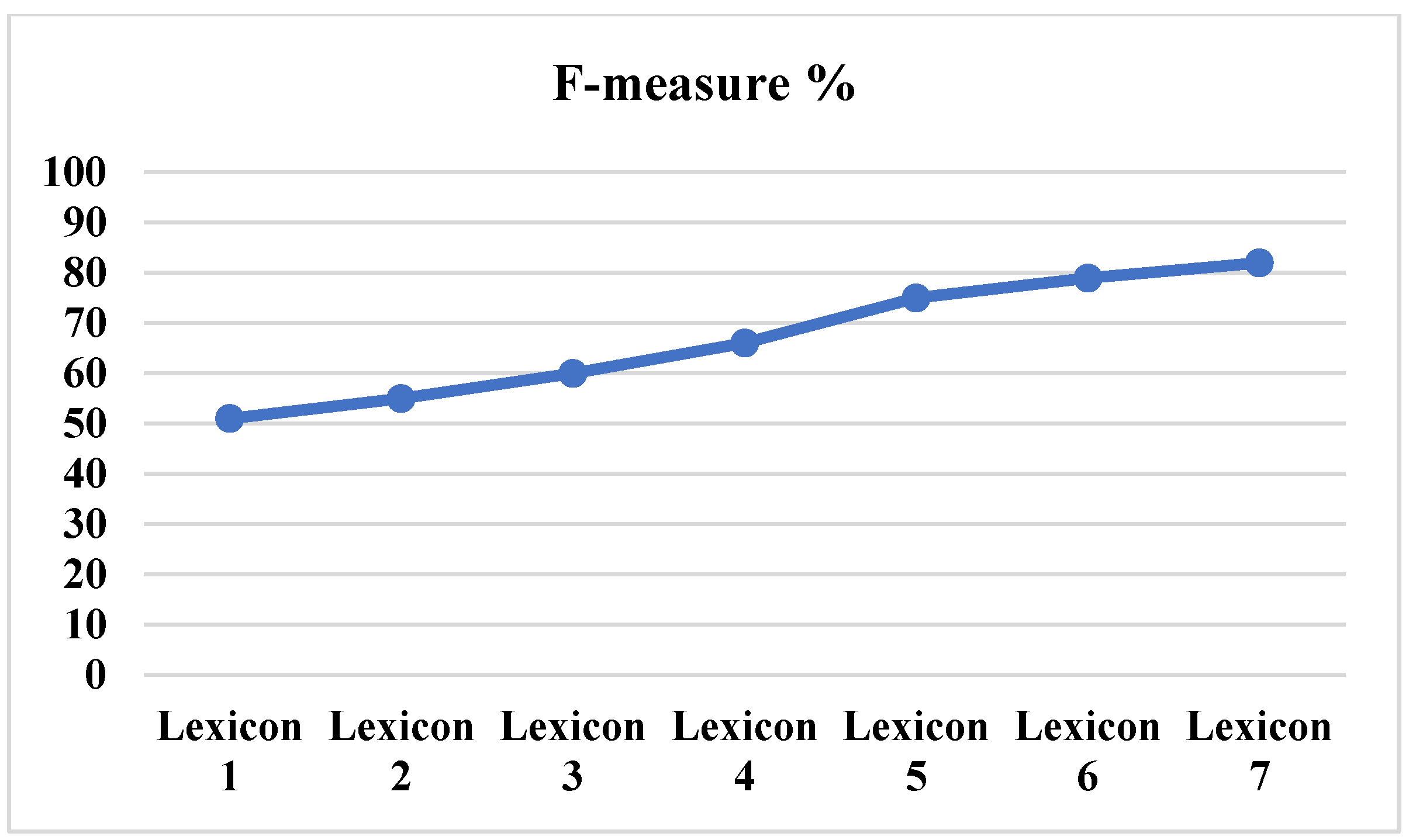
In the next stage, the numerical representation for each sentence was obtained. The processed dataset was submitted words-wise to an embedding pre-trained model BERT. After that, SentiWordNet, TextBlob, VADER, UMLS, and statistical techniques were used to develop a specialized vocabulary (medical domain) that determined the polarity of each sentence. Various sizes of the lexicon (number of terms) were also examined to test this method’s reliability [57]. The lexicon’s capacities were also evaluated with different sizes of lexicons to investigate whether the largest or smallest lexicon of sentiment can produce better results [58]. The largest lexicon produced the highest performance, and the smallest lexicon resulted poorly. Figure 6 compares the obtained results relying on the number of words in each lexicon, indicating the values of lexicons 1,2, 3, 4, 5, 6, and 7 are 10.000, 20.000, 30.000, 40.000, 50.000, 60.000, and 70.000, respectively.
After creating the lexicons, the ratio of the sentiments in assigning the polarity was non-equivalent, indicating the model over-fit on the unbalanced dataset. To solve these issues, SMOTE-OSS-CNN (One-Side-Selection) and (Condensed Nearest Neighbors) were proposed for the imbalanced datasets following the balance of the number of samples for all classes in the dataset. Balancing was accomplished by generating the synthetic minority samples so that the number of samples for the minority class was almost equal to that of the majority class. Consequently, the models achieved a high accuracy using the SMOTE-OSS-CNN approach, producing synthetic samples of the minority class [59]. In brief, the proposed models achieved a high level of accuracy when the SMOTE-OSS-CNN approach was employed to produce the artificial samples of the minority class. The binary classification was performed as the first experiment of the proposed method, which was achieved for four cases of illness: asthma with neutral and positive labels, asthma with neutral and negative labels, obesity with neutral and positive labels, and obesity with neutral and negative labels.
5. Baselines
To validate the performance of the proposed solution, this paper compares it with state-of-the-art techniques; all the basslines have been experimented on based on the datasets that were applied in this paper.
- IMN-GloVe is a collaborating MTL method for SE, ASC, and ATE, which can be applied at both the token word and document levels. IMN proposed a message transfer system that may change across tasks via shared latent variables. MMS compares their findings utilizing BERT-large for a pre-trained linguistic model for a fair comparison.
- BERT-single, BERT is a primary component of our BERT-based proposed solution. To illustrate the effectiveness of the auxiliary sentence, this paper also compared it with BERT-single, where ACSA is regarded as a text classification problem.
- AEN-BERT is an attentional encoder network for the ATSA task, which models context and target through an attention-based encoder. AEN-BERT is the pre-trained model BERT fine-tuning to tackle ATSA tasks. In our experiment, this paper adopts it to tackle the ACSA task.
- BERT-SPC, a BERT-based approach, introduced concatenating the aspect and sentence in one long text, then fine-tuned BERT to address the ATSA task. In our experiment, this paper adopts it to tackle the ACSA task.
- LCF-BERT proposed a local context focus mechanism that used the context features mask and context dynamic weight layer to capture the local aspect context. An addition layer based on BERT is applied to exploit the connection between the local and global context.
- BERT-Pair, a BERT-based fine-tuning model that considered the aspect category manually annotated as an auxiliary sentence. It introduced different variants to convert ACSA to sentence-pair classification tasks, such as question answering and natural language inference.
6. Evaluation Metrics
The suggested model in this work has been evaluated using recall, precision, accuracy, and F-measure (F1). The performance and efficacy of a given approach model are assessed using a variety of measures. Because not all measures are appropriate for a particular problem, a model is crucial in this last stage of development. Sometimes, a new assessment metric can be offered to assess the final approach. The measurements chosen may impact how a model’s effectiveness and performance are compared and evaluated. A simple confusion matrix is a two-by-two that lists all incorrect and correct patterns predicted by a classifier model [60]. For instance, True Negative (TN) shows the number of negative samples that the classifier correctly predicted as negative, False Positive (FP) shows the number of negative samples that the classifier incorrectly predicted as positive, and so on. False Negative (FN) shows how many positive samples the classifier incorrectly identified as negative, and True Positive (TP) shows how many positive samples the classifier correctly predicted as positive [61].
MMS applies BERT-large with 1024 hidden dimensions. The maximum number of sentences that may be entered is 100. To update MMS, Adam Optimizer is utilized. The batch size is 64. The learning rate of the linear layers and BERT-large on the maximum of BERT-large is equal to 8 × 10⁻⁵ and 4 × 10⁻⁵, respectively. The 8 × 10⁻⁵ is referred to . The method applied a threshold , lower (L%) and upper (U%), and limits of doubts for the objects brought to the student model by MMS are presented in Table 3. In Algorithm 1, the total training epoch is 500, and is set to 2.
7. Results
The key findings of the suggested MMS are shown in Table 5. Since MMS is a self-training technique, this paper investigates how well it performs with various quantities of manually annotated data. It is important to note that while this paper reported MMS performance using the datasets in 10%, 20%, and 40% with benchmarking baselines, all labeled data from the corresponding dataset are shown in Table 5. Additionally, MMS has been evaluated using additional unlabeled dataset augmentation with 70% and 100% of the data. Between 70% and 100% of labeled data, respectively, have been used in both settings. The introduction of the unlabeled dataset augmentation is intended to provide extra pseudo-labeled data to aid in learning the student technique and the meta-weigher. More labeled data for MMS leads to increases in all MMS F1 metrics of various sub-tasks, as shown in Table 5. In terms of ABSA-F1, which has just 30% labeled data, this paper suggested MMS performs better than the state-of-the-art techniques. In addition, MMS sightly best performs the state-of-the-art method BERT-Pair in the Asthma and Obesity datasets, with only 40% labeled data. The 40% labeled data of Asthma has been adopted, and ABSA-F1 of MMS is lower than the results of full-data supervised AEN-BERT. This conclusion results from the magnitude of the asthma data being less than half that of the obesity data. The produced pseudo data may be excessively noisy from an unreliable instructor model, making it insufficient to train a robust instructor model to direct a student model.
Next, MMS uses additional unlabeled data from another dataset for self-training together with 70% and 100% of the annotated data from the datasets for Obesity and Asthma as labeled data. The Dataset section describes the extra unlabeled data that was used. The reductions in Asthma are visible with more labeled data, whereas the improvements in Obesity begin to be restricted. In Asthma, for example, ABSA-F1 measurements rise by 1.05% (40% vs. 70%) and 1.71% (70% vs. 100%). In Obesity, the equivalent increases are 0.75% (40% vs. 70%) and 0.77% (70% vs. 100%). These findings suggest that MMS can, to some extent, decrease the need for labeled data.
To summarize, MMS may obtain equivalent outcomes with only 40% labeled data compared to the strongest baselines in each dataset. MMS uses more stringent data choices to prevent noise effects when using 70% and 100% labeled data. In such cases, where there is a lack of data, MMS can obtain equivalent outcomes with only 50% labeled data. MMS uses more stringent data choices to prevent noise effects when using 70% and 100% labeled data. Because the issue of inadequate data is not evident in this situation, MMS creates fewer pseudo-labels and focuses on re-weighting data instances in . Then, the final improvement of MMS is 1.41% compared with the BERT-Pair method in Obesity and 0.84% with LCF-BERT in Asthma.
More labeled data for MMS, all MMS F1 scores of distinct sub-tasks are generally growing. With only 20% labeled data from ABSA-F1, this paper suggested MMS beats IMN-GloVe in all sub-tasks. In the same settings, MMS is comparable to the performance of LCF-BERT in Asthma and Obesity datasets, achieving improved results in Asthma. By applying the same BERT encoder and 40% labeled data, MMS can attain the enhancements of around 6% ABSA-F1 for Asthma and approximately 1% ABSA-F1 for Obesity, compared with the state-of-the-art methods. Following all baselines, this paper considers the first sentiment label predicted for an aspect phrase to be an ASC result, and this paper excludes conflicting sentiment labels from the ASC subtask. This exclusion may cause the ratio sum in ASC to be less than 100%. Additionally, as mentioned earlier, this paper assigns an enhanced dataset for each dataset to further investigate MMS’s data usage.
On the other hand, the effects of the quantity of data with and without labels. This paragraph investigates the effects of various amounts of annotated data on MMS. The impacts of incorporating and removing unlabeled data on model performance are first contrasted (see Table 5). All models often demonstrate the growing F1 measures by using additional labeled data. Across all of the used labeled data ratios, MMS (including unlabeled data) may consistently enhance the ABSA-F1 measurements by 10% to 40%. The largest discrepancy between MMS labeled data and unlabeled data emerges when employing 10% labeled data in Asthma, accounting for 4.10%. The greatest noticeable gains for Obesity are provided by 1.10% with 40% labeled data. MSM with 10% tagged data shows a modest improvement for the obesity and asthma datasets. The improvement is visible when utilizing more than 20% tagged data. This is due to the difficulty in managing a workable instructor model with only 10% labeled data. Effective initialization of the instructor model is required for MMS to prevent progressive drift.
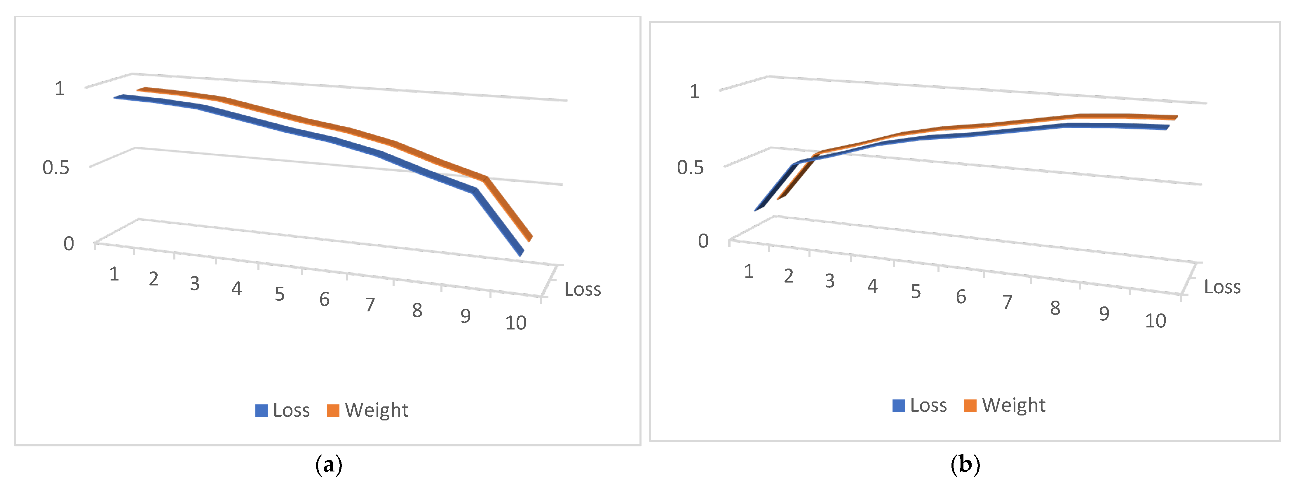
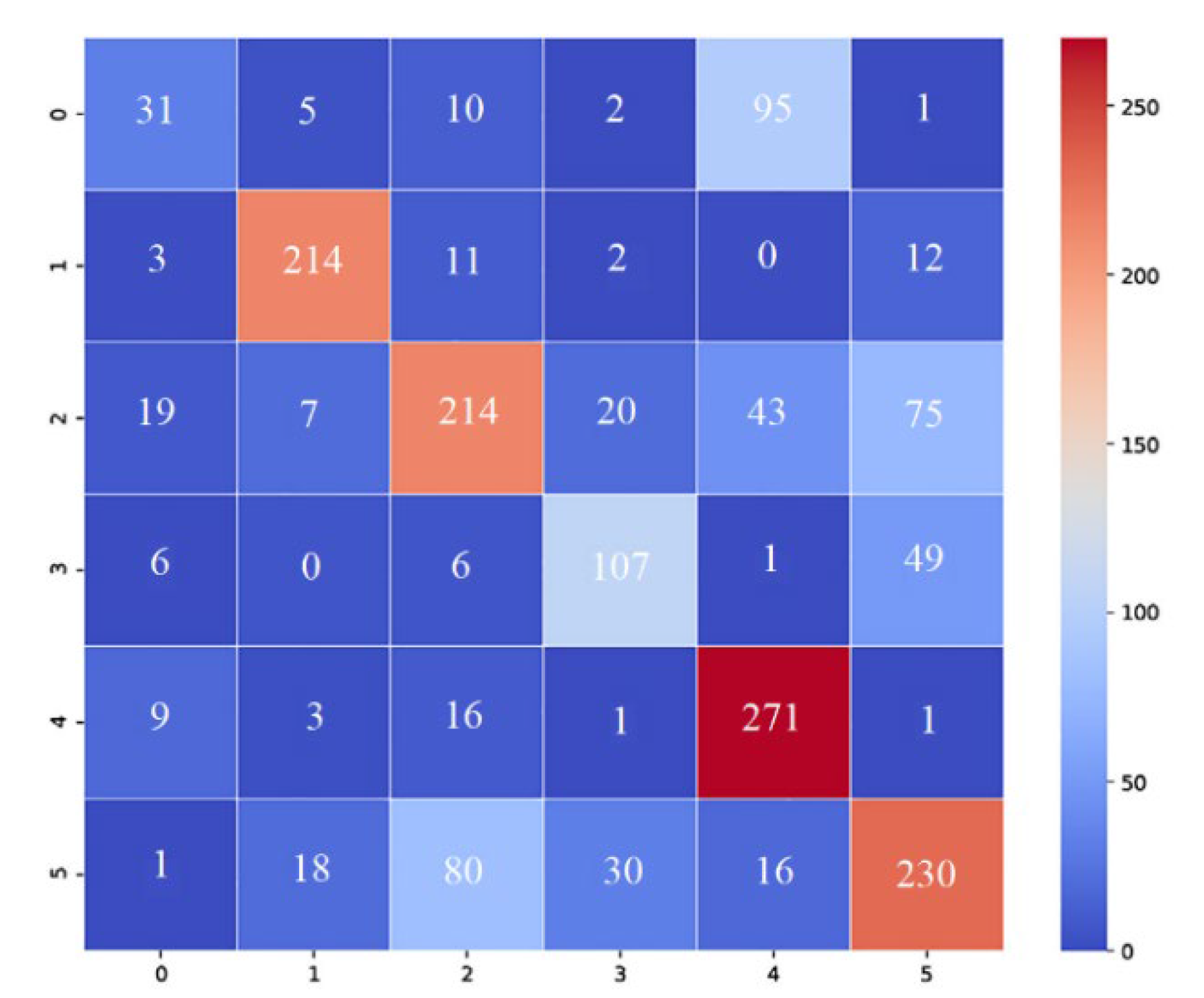
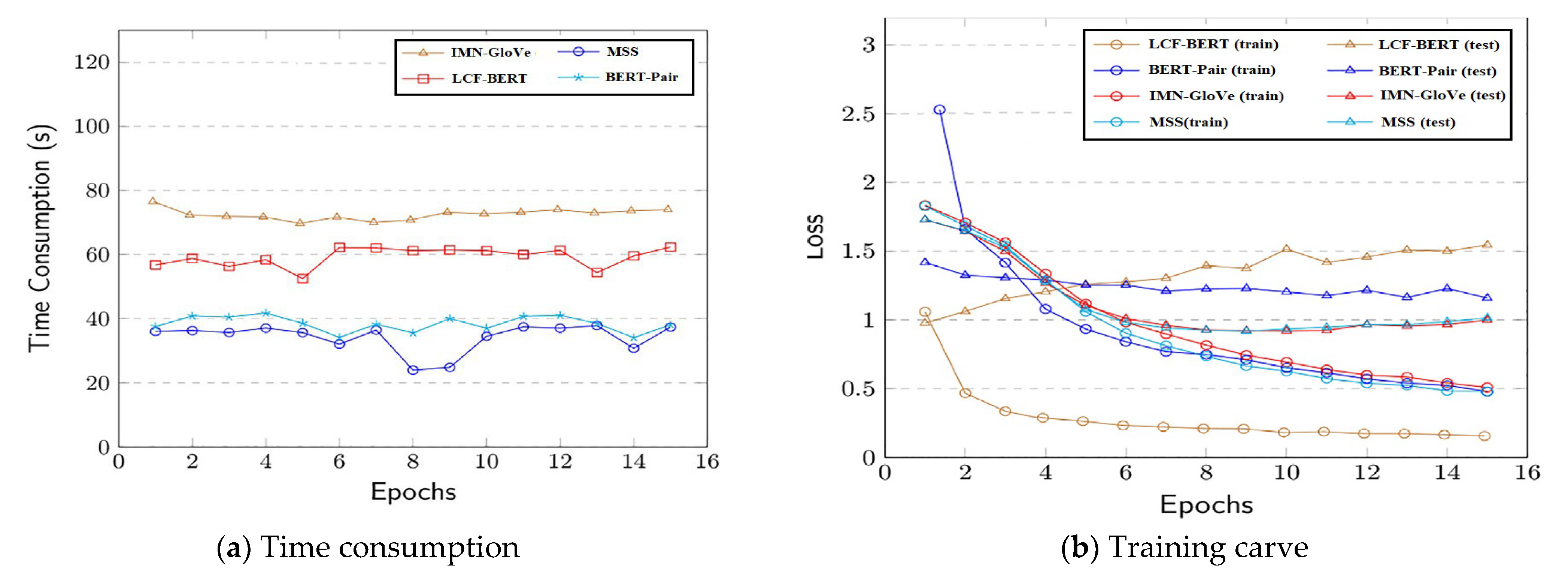
This paper illustrates the produced weights and contrasts them with different common weighting techniques since the MMS meta-weigher seeks to automatically learn various weighting strategies under various scenarios (weighers). Weighers’ inputs are virtual losses in the range of 0 to 10. The virtual losses are uniformly distributed, automatically created numbers. These losses replicate all potential inputs to our weighers within a reasonable range, which helps visualize the learned distribution of weighers. Afterward, several weighers are fed the losses. For more information, see Figure 7, including four different cases (a) to (d). The explicit mathematical functions are manually used in the construction of the weighers. The weigher is this paper’s suggested meta-weigher, which is trained using various ABSA sub-tasks and datasets. We take advantage of visualization to reveal certain details about the suggested model. To illustrate the effectiveness of our MMS model, this paper first shows the confusion matrix as a heat map. Figure 8 displays the MMS heat maps on the DS dataset. Overall, the sentiment classes and the performance of our model are balanced. In terms of convergence capability, the quantity of trainable parameters, and training time, our suggested model outperforms IMN-GloVe. Our models require a great deal less training time as compared to BERT-Pair. As a result, our model learns more rapidly than its equivalent, as seen in Figure 9a, where training time is recorded on a single NVIDIA Quadro M5000. Our MMS model is more parameter-efficient and takes less time to train, whether the context is global or local. The training curve is displayed with training and testing losses in Figure 9b. For all the compared models, this paper uses the same loss function. While LCF-BERT is prone to overfitting, in this paper, MMS converges as quickly as its competitors.
8. Conclusions
In conclusion, this research proposes a multi-task approach for aspect-based sentiment analysis, utilizing deep neural network models for sentiment detection. To address the issue of insufficient and unbalanced data in the MABSA task, the SMOTE-OSS-CNN, and meta-based self-training approach MMS are suggested. MMS contains the meta-weightier, the student model, and the instructor model, and a 3-step meta-updating technique is suggested to avoid noise in the automatically labeled data. Overall, this study has implications for discharge summary sentiment analysis.
Future work will involve dealing with numerous sequence labeling jobs under more challenging low-data conditions. Moreover, this paper intends to explore data augmentation to address imbalanced data to increase performance stance detection. Additionally, feature extraction is required for greater contextual information, for example, information on the aforementioned discharge summary, discharge in the same thread, and disease connection networks to enhance sentiment stance detection on discharge summary.
Funding
This work was supported by the National Natural Science Foundation of China (Grant No. U1811262).
Institutional Review Board Statement
Not applicable.
Informed Consent Statement
Not applicable.
Data Availability Statement
The raw data supporting the conclusions of this article will be made available by the authors on request, medical information need the permission to get it.
Acknowledgments
We are very grateful to the Chinese Scholarship Council (CSC) for providing us with financial and moral support.
Conflicts of Interest
The authors declare no conflict of interest.
References
- Waheeb, S.A.; Ahmed Khan, N.; Chen, B.; Shang, X. Machine learning based sentiment text classification for evaluating treatment quality of discharge summary. Information 2020, 11, 281. [Google Scholar] [CrossRef]
- Waheeb, S.A.; Khan, N.A.; Shang, X. An efficient sentiment analysis based deep learning classification model to evaluate treatment quality. Malays. J. Comput. Sci. 2022, 35, 1–20. [Google Scholar] [CrossRef]
- Li, Y.; Lin, Y.; Lin, Y.; Chang, L.; Zhang, H. A span-sharing joint extraction framework for harvesting aspect sentiment triplets. Knowl. Based Syst. 2022, 242, 108366. [Google Scholar] [CrossRef]
- Chen, F.; Yang, Z.; Huang, Y. A multi-task learning framework for end-to-end aspect sentiment triplet extraction. Neurocomputing 2022, 479, 12–21. [Google Scholar] [CrossRef]
- Wei, S.; Zhu, G.; Sun, Z.; Li, X.; Weng, T. GP-GCN: Global features of orthogonal projection and local dependency fused graph convolutional networks for aspect-level sentiment classification. Connect. Sci. 2022, 34, 1785–1806. [Google Scholar] [CrossRef]
- Nagra, A.A.; Alissa, K.; Ghazal, T.; Saigeeta, S.; Asif, M.M.; Fawad, M. Deep Sentiments Analysis for Roman Urdu Dataset Using Faster Recurrent Convolutional Neural Network Model. Appl. Artif. Intell. 2022, 36, 2123094. [Google Scholar] [CrossRef]
- Yang, L.; Na, J.-C.; Yu, J. Cross-Modal Multitask Transformer for End-to-End Multimodal Aspect-Based Sentiment Analysis. Inf. Process. Manag. 2022, 59, 103038. [Google Scholar] [CrossRef]
- Blanco, A.; Remmer, S.; Pérez, A. Implementation of specialised attention mechanisms: ICD-10 classification of Gastrointestinal discharge summaries in English, Spanish and Swedish. J. Biomed. Inform. 2022, 130, 104050. [Google Scholar] [CrossRef]
- Trigueros, O.; Blanco, A.; Lebeña, N.; Casillas, A.; Pérez, A. Explainable ICD multi-label classification of EHRs in Spanish with convolutional attention. Int. J. Med. Inform. 2022, 157, 104615. [Google Scholar] [CrossRef]
- Wu, Y.; Zeng, M.; Yu, Y.; Li, Y.; Li, M. A Pseudo Label-wise Attention Network for Automatic ICD Coding. IEEE J. Biomed. Health Inform. 2022, 26, 5201–5212. [Google Scholar] [CrossRef]
- Aviles-Rivero, A.; Sellars, P.; Schönlieb, C.-B.; Papadakis, N. GraphXCOVID: Explainable deep graph diffusion pseudo-labelling for identifying COVID-19 on chest X-rays. Pattern Recognit. 2022, 122, 108274. [Google Scholar] [CrossRef] [PubMed]
- Momma, M.; Dong, C.; Liu, J. A multi-objective/multi-task learning framework induced by Pareto stationarity. In Proceedings of the International Conference on Machine Learning, Baltimore, MD, USA, 17–23 July 2022; pp. 15895–15907. [Google Scholar]
- Yu, W.; Xu, H. Co-attentive multi-task convolutional neural network for facial expression recognition. Pattern Recognit. 2022, 123, 108401. [Google Scholar] [CrossRef]
- Zhang, Z.; Yu, W.; Yu, M.; Guo, Z.; Jiang, M. A survey of multi-task learning in natural language processing: Regarding task relatedness and training methods. arXiv 2022, arXiv:2204.03508. [Google Scholar]
- Han, S.; Mao, R.; Cambria, E. Hierarchical Attention Network for Explainable Depression Detection on Twitter Aided by Metaphor Concept Mappings. arXiv 2022, arXiv:2209.07494. [Google Scholar]
- Mao, R.; Li, X. Bridging towers of multi-task learning with a gating mechanism for aspect-based sentiment analysis and sequential metaphor identification. In Proceedings of the AAAI Conference on Artificial Intelligence, Washington, DC, USA, 7–14 February 2023; pp. 13534–13542. [Google Scholar]
- Wang, X.; Xu, G.; Zhang, Z. End-to-end aspect-based sentiment analysis with hierarchical multi-task learning. Neurocomputing 2021, 455, 178–188. [Google Scholar] [CrossRef]
- Chen, Z.; Qian, T. Relation-aware collaborative learning for unified aspect-based sentiment analysis. In Proceedings of the 58th Annual Meeting of the Association for Computational Linguistics, Online, 5–10 July 2020; pp. 3685–3694. [Google Scholar]
- Chen, S.; Shi, X.; Li, J.; Wu, S.; Fei, H.; Li, F.; Ji, D. Joint Alignment of Multi-Task Feature and Label Spaces for Emotion Cause Pair Extraction. arXiv 2022, arXiv:2209.04112. [Google Scholar]
- Kim, M.; Kang, P. Text Embedding Augmentation Based on Retraining with Pseudo-Labeled Adversarial Embedding. IEEE Access 2022, 10, 8363–8376. [Google Scholar] [CrossRef]
- Xu, L.; Lu, X.; Yuan, C. Few-Shot Learning for Chinese NLP Tasks. In Proceedings of the CCF International Conference on Natural Language Processing and Chinese Computing, Guilin, China, 24–25 September 2022; pp. 412–421. [Google Scholar]
- Chen, Y.; Zhang, Y.; Zhang, C. Revisiting Self-Training for Few-Shot Learning of Language Model. arXiv 2021, arXiv:2110.01256v1. [Google Scholar]
- Du, J.; Grave, E.; Gunel, B.; Chaudhary, V. Self-training improves pre-training for natural language understanding. arXiv 2020, arXiv:2010.02194. [Google Scholar]
- Wang, Y.; Mukherjee, S.; Chu, H. Meta self-training for few-shot neural sequence labeling. In Proceedings of the 27th ACM SIGKDD Conference on Knowledge Discovery & Data Mining, New York, NY, USA, 14–18 August 2021; pp. 1737–1747. [Google Scholar]
- Jayasinghe, K. Bootstrapping Sinhala Named Entities for NLP Applications. Ph.D Thesis, University of Colombo School of Computing, Sri Lanka, 2021. Available online: https://dl.ucsc.cmb.ac.lk/jspui/handle/123456789/4195 (accessed on 28 May 2023).
- Jin, Q.; Yuan, M.; Wang, H.; Wang, M.; Song, Z. Deep active learning models for imbalanced image classification. Knowl. Based Syst. 2022, 257, 109817. [Google Scholar] [CrossRef]
- Ahmed, U.; Lin, J.C.-W.; Srivastava, G. A resource allocation deep active learning based on load balancer for network intrusion detection in SDN sensors. Comput. Commun. 2022, 184, 56–63. [Google Scholar] [CrossRef]
- Alshemali, B.; Kalita, J. Improving the reliability of deep neural networks in NLP: A review. Knowl. Based Syst. 2020, 191, 105210. [Google Scholar] [CrossRef]
- Joshi, V.; Ghongade, R.; Joshi, A.; Kulkarni, R. Deep BiLSTM neural network model for emotion detection using cross-dataset approach. Biomed. Signal Process. Control 2022, 73, 103407. [Google Scholar] [CrossRef]
- Khan, N.S.; Ghani, M.S. A survey of deep learning based models for human activity recognition. Wirel. Pers. Commun. 2021, 120, 1593–1635. [Google Scholar] [CrossRef]
- Ke, J.; Wang, L.; Ye, A. Combating Multi-level Adversarial Text with Pruning based Adversarial Training. In Proceedings of the 2022 International Joint Conference on Neural Networks (IJCNN), Padua, Italy, 18–23 July 2022; pp. 1–8. [Google Scholar]
- Mokhosi, R.; Shikali, C.; Qin, Z.; Liu, Q.J.C.S. Maximal activation weighted memory for aspect based sentiment analysis. Comput. Speech Lang. 2022, 76, 101402. [Google Scholar] [CrossRef]
- Miao, S.; Lu, M. Targeted Aspect-Based Sentiment Analysis by Utilizing Dynamic Aspect Representation. In Proceedings of the International Conference on Artificial Neural Networks, Bristol, UK, 6–9 September 2022; pp. 647–659. [Google Scholar]
- He, K.; Mao, R.; Gong, T. Meta-based self-training and re-weighting for aspect-based sentiment analysis. IEEE Trans. Affect. Comput. 2022, 47, 1–13. [Google Scholar] [CrossRef]
- Zhang, W.; Li, X.; Deng, Y.; Bing, L.; Lam, W. A Survey on Aspect-Based Sentiment Analysis: Tasks, Methods, and Challenges. arXiv 2022, arXiv:2203.01054. [Google Scholar] [CrossRef]
- Liu, W.; Hu, J.; Du, S.; Chen, H.; Teng, F. A Method of Sharing Sentence Vectors for Opinion Triplet Extraction. Neural Process. Lett. 2022, 55, 1–22. [Google Scholar] [CrossRef]
- Liang, B.; Su, H.; Gui, L.; Cambria, E.; Xu, R. Aspect-based sentiment analysis via affective knowledge enhanced graph convolutional networks. Knowl. Based Syst. 2022, 235, 107643. [Google Scholar] [CrossRef]
- Zhou, T.; Law, K.M. Semantic Relatedness Enhanced Graph Network for aspect category sentiment analysis. Expert Syst. Appl. 2022, 195, 116560. [Google Scholar] [CrossRef]
- Zhang, Y.; Peng, T.; Han, R.; Han, J.; Yue, L.; Liu, L. Synchronously tracking entities and relations in a syntax-aware parallel architecture for aspect-opinion pair extraction. Appl. Intell. 2022, 13, 15210–15225. [Google Scholar] [CrossRef]
- Ge, L.; Li, J. MTHGAT: A Neural Multi-task Model for Aspect Category Detection and Aspect Term Sentiment Analysis on Restaurant Reviews. In Proceedings of the International Conference on Artificial Neural Networks, Munich, Germany, 17–19 September 2019; pp. 270–281. [Google Scholar]
- Zhao, Z.; Tang, M.; Tang, W. Graph convolutional network with multiple weight mechanisms for aspect-based sentiment analysis. Neurocomputing 2022, 23, 157. [Google Scholar] [CrossRef]
- Li, G.; Kong, B.; Li, J.; Fan, H.; Zhang, J.; An, Y.; Yang, Z.; Danz, S.; Fan, J. A BERT-based Text Sentiment Classification Algorithm through Web Data. In Proceedings of the 2022 International Conference on Computer Engineering and Artificial Intelligence (ICCEAI), Shijiazhuang, China, 22–24 July 2022; pp. 477–481. [Google Scholar]
- El-Hasnony, I.; Elzeki, O.; Alshehri, A. Multi-label active learning-based machine learning model for heart disease prediction. Sensors 2022, 22, 1184. [Google Scholar] [CrossRef] [PubMed]
- Zhuang, Q.; Dai, Z.; Wu, J. Deep Active Learning Framework for Lymph Node Metastasis Prediction in Medical Support System. Comput. Intell. Neurosci. 2022, 2022, 4601696. [Google Scholar] [CrossRef] [PubMed]
- Peng, X.; Jin, X.; Duan, S.; Sankavaram, C. Active Learning Assisted Semi-Supervised Learning for Fault Detection and Diagnostics with Imbalanced Dataset. IISE Trans. 2022, 55, 672–686. [Google Scholar] [CrossRef]
- Liu, Y.; Ott, M.; Goyal, N.; Du, J.; Joshi, M.; Chen, D.; Levy, O.; Lewis, M.; Zettlemoyer, L.; Stoyanov, V.J.A.P.A. Roberta: A robustly optimized bert pretraining approach. arXiv 2019, arXiv:1907.11692. [Google Scholar]
- Sanh, V.; Debut, L.; Chaumond, J.; Wolf, T.J.A.P.A. DistilBERT, a distilled version of BERT: Smaller, faster, cheaper and lighter. arXiv 2019, arXiv:1910.01108. [Google Scholar]
- Cañete, J.; Chaperon, G.; Fuentes, R.; Ho, J.H.; Kang, H.; Pérez, J. Spanish pre-trained bert model and evaluation data. arXiv 2020, arXiv:2308.02976. [Google Scholar]
- Palani, S.; Rajagopal, P.; Pancholi, S.J.A.P.A. T-BERT--Model for Sentiment Analysis of Micro-blogs Integrating Topic Model and BERT. arXiv 2021, arXiv:2106.01097. [Google Scholar]
- Lee, J.-S.; Hsiang, J.J.A.P.A. Patentbert: Patent classification with fine-tuning a pre-trained bert model. arXiv 2019, arXiv:1906.02124. [Google Scholar]
- Guo, Y.; Zhou, D.; Li, W.; Cao, J. Deep multi-scale Gaussian residual networks for contextual-aware translation initiation site recognition. Expert Syst. Appl. 2022, 207, 118004. [Google Scholar] [CrossRef]
- Pires, T.; Schlinger, E.; Garrette, D.J.A.P.A. How multilingual is multilingual bert? arXiv 2019, arXiv:1906.01502. [Google Scholar]
- Mounica, B.; Lavanya, K. Feature selection method on twitter dataset with part-of-speech (PoS) pattern applied to traffic analysis. Int. J. Syst. Assur. Eng. Manag. 2022. [Google Scholar] [CrossRef]
- Chanda, A.K.; Bai, T.; Yang, Z.; Vucetic, S. Improving medical term embeddings using UMLS Metathesaurus. BMC Med. Inform. Decis. Mak. 2022, 22, 114. [Google Scholar] [CrossRef] [PubMed]
- Tan, J.S.; Chia, W.C. Research Output to Industry Use: A Readiness Study for Topic Modelling with Sentiment Analysis. In Proceedings of the 8th International Conference on Computational Science and Technology, Labuan, Malaysia, 28–29 August 2021; pp. 13–25. [Google Scholar]
- Gupta, I.; Madan, T.K.; Singh, S.; Singh, A.K. HiSA-SMFM: Historical and Sentiment Analysis based Stock Market Forecasting Model. arXiv 2022, arXiv:2203.08143. [Google Scholar]
- Zaghir, J.; Rodrigues, J.F., Jr.; Goeuriot, L.; Amer-Yahia, S. Real-world Patient Trajectory Prediction from Clinical Notes Using Artificial Neural Networks and UMLS-Based Extraction of Concepts. J. Healthc. Inform. Res. 2021, 4, 474–496. [Google Scholar] [CrossRef] [PubMed]
- Bravo-Marquez, F.; Khanchandani, A.; Pfahringer, B.J. Incremental Word Vectors for Time-Evolving Sentiment Lexicon Induction. Cogn. Comput. 2021, 14, 425–441. [Google Scholar] [CrossRef]
- Rupapara, V.; Rustam, F.; Shahzad, H.F.; Mehmood, A.; Ashraf, I.; Choi, G.S.J.I.A. Impact of SMOTE on Imbalanced Text Features for Toxic Comments Classification using RVVC Model. IEEE Access 2021, 9, 78621–78634. [Google Scholar] [CrossRef]
- Li, J.; Sun, H.; Li, J. Beyond confusion matrix: Learning from multiple annotators with awareness of instance features. Mach. Learn. 2022, 112, 1053–1075. [Google Scholar] [CrossRef]
- Theissler, A.; Thomas, M.; Burch, M.; Gerschner, F. ConfusionVis: Comparative evaluation and selection of multi-class classifiers based on confusion matrices. Knowl. Based Syst. 2022, 247, 108651. [Google Scholar] [CrossRef]
Figure 1.
The outline suggested a meta-weigher with a meta-based self-training method (MMS). The display of various data streams uses various color schemes.
Figure 1.
The outline suggested a meta-weigher with a meta-based self-training method (MMS). The display of various data streams uses various color schemes.

Figure 2.
Demonstrates how the student model and meta-weigher are updated by MMS from the first-time step to the second-time step .
Figure 2.
Demonstrates how the student model and meta-weigher are updated by MMS from the first-time step to the second-time step .

Figure 3.
An overview of the ML when applied in AL.

Figure 4.
The word clouds frequently occurred in sentiment terms in medical documents.

Figure 5.
The steps of the proposed solution.

Figure 6.
The size-dependent performance of each sentiment lexicon.

Figure 7.
The representation of weights learned via different techniques. Illustration of the different weights educated by the meta-weigher of MMS on SE, ASC, and ATE of Asthma and Obesity datasets.
Figure 7.
The representation of weights learned via different techniques. Illustration of the different weights educated by the meta-weigher of MMS on SE, ASC, and ATE of Asthma and Obesity datasets.


Figure 8.
Confusion matrix for MMS model in heat map form.

Figure 9.
The training curve and time use were recorded using the DS dataset on a single GPU.


Table 1.
The i2b2 obesity corpus statistics.
| Diseases | Absent | Present | Unmentioned | Questionable | Total |
|---|---|---|---|---|---|
| Asthma | 1 | 75 | 529 | 1 | 606 |
| CHF | 7 | 239 | 344 | 0 | 589 |
| CAD | 16 | 331 | 240 | 4 | 591 |
| Obesity | 3 | 245 | 354 | 4 | 606 |
| Diabetes | 12 | 396 | 181 | 6 | 595 |
| Depression | 0 | 90 | 519 | 0 | 609 |
| GERD | 1 | 98 | 500 | 3 | 602 |
| Gallstones | 3 | 93 | 513 | 0 | 609 |
| Hypercholesterolemia | 9 | 246 | 343 | 1 | 599 |
| Gout | 0 | 73 | 534 | 2 | 609 |
| Hypertriglyceridemia | 0 | 15 | 594 | 0 | 609 |
| Hypertension | 10 | 441 | 149 | 0 | 600 |
| OSA | 0 | 88 | 510 | 7 | 604 |
| OA | 0 | 89 | 513 | 0 | 602 |
| Venous Insufficiency | 0 | 14 | 592 | 0 | 606 |
| PVD | 0 | 83 | 525 | 0 | 608 |
| Sum | 62 | 2616 | 6940 | 28 | 9644 |
Table 2.
The gold standard corpus statistics.
| Diseases | Very Positive | Positive | Neutral | Negative | Very Negative | Total |
|---|---|---|---|---|---|---|
| Obesity | 141 | 215 | 180 | 41 | 29 | 606 |
| Asthma | 213 | 150 | 211 | 21 | 11 | 606 |
Table 3.
The percentage of tags ratio refers to the various tags for each sub-task. For the SE and ATE sub-tasks, it shows the tags O, I, and B for all tag percentages. For the ASC sub-task, it shows the tags ratio of very positive, positive, neutral, negative, and very negative.
Table 3.
The percentage of tags ratio refers to the various tags for each sub-task. For the SE and ATE sub-tasks, it shows the tags O, I, and B for all tag percentages. For the ASC sub-task, it shows the tags ratio of very positive, positive, neutral, negative, and very negative.
| Dataset | Statistics | Training | Validation | Testing |
|---|---|---|---|---|
| Obesity | No. Sentence | 2155 | 510 | 990 |
| No. Token | 31,120 | 7240 | 10,560 | |
| Aspect labels (%) | 10.93 | 9.99 | 13.20 | |
| Opinion labels (%) | 9.02 | 7.29 | 8.90 | |
| The ratio of tags (SE) (%) | 7/2/77 | 7/3/79 | 8/3/77 | |
| The ratio of tags (ATE) (%) | 9/2/89 | 9/2/11 | 8/2/88 | |
| The ratio of tags (ASC) (%) | 8/3/3/4/6 | 8/3/3/4/4 | 9/3/3/4/5 | |
| Asthma | No. Sentence | 1160 | 220 | 870 |
| No. Token | 3090 | 8210 | 9620 | |
| Aspect labels (%) | 9.89 | 10.01 | 12.41 | |
| Opinion labels (%) | 9.15 | 7.40 | 8.97 | |
| The ratio of tags (SE) (%) | 9/3/80 | 9/4/90 | 9/4/79 | |
| The ratio of tags (ATE) (%) | 8/3/90 | 9/3/12 | 9/2/80 | |
| The ratio of tags (ASC) (%) | 8/3/3/4/6 | 8/3/3/4/7 | 9/3/3/4/6 |
Table 4.
The values of the fine-tuned Hyperparameters.
| Hyperparameter | Value |
|---|---|
| Maximum sequence length | 128 |
| Parameters | 110 M |
| Hidden size | 768 |
| Learning rate | 0.00003 |
| Epochs | 8 |
| Gradient accumulation steps | 16 |
| Attention heads | 12 |
| Hidden layers | 12 |
Table 5.
The comparative results of the aspect category polarity on Asthma and Obesity datasets were measured by the F1 metric with multi-sub tasks. Some results of the state-of-the-art methods are retrieved from the original papers, while the others are our implementation. The best scores are highlighted in bold.
| Model | Asthma | Obesity | ||||||
|---|---|---|---|---|---|---|---|---|
| SE-F1 | ASC-F1 | ATE-F1 | ABSA-F1 | SE-F1 | ASC-F1 | ATE-F1 | ABSA-F1 | |
| IMN-GloVe | 82.0% | 84.0% | 87.3% | 88.67% | 86.9% | 88.56% | 85.5% | 93.3% |
| BERT-Single | 85.14% | 87.25% | 90.14% | 90.07% | 86.87% | 87.98% | 86,68% | 92.06% |
| AEN-BERT | 88.3% | 89.9% | 93.83% | 80.74% | 88.08% | 90.0% | 92.28% | 93.93% |
| BERT-SPC | 89.9% | 91.6% | 93.3% | 90.11% | 88.83% | 88.55% | 92.51% | 93.89% |
| LCF-BERT | 88.7% | 91.1% | 92.8% | 91.72% | 89.3% | 89.86% | 93.6% | 94.4% |
| BERT-Pair | 91.37% | 91.1% | 92.67% | 93.60% | 88.7% | 86.82% | 92.1% | 92.4% |
| MMS (our) | 87.85% | 89.05% | 95.94% | 96.4% | 94.45% | 86.64% | 89.35% | 93.0% |
| MMS (10%) | 87.92% | 84.61% | 85.26% | 92.74% | 91.04% | 86.24% | 88.58% | 86.4% |
| MMS (20%) | 91.82% | 89.25% | 89.87% | 93.76% | 92.78% | 89.07% | 90.89% | 89.05% |
| MMS (40%) | 92.07% | 90.86% | 91.25% | 93.39% | 92.78% | 90.24% | 91.54% | 89.35% |
| MMS (70%) | 93.78% | 91.37% | 91.77% | 90.07% | 93.04% | 89.95% | 91.47% | 93.60% |
| MMS (100%) | 91.37% | 91.77% | 86.82% | 96.90% | 93.72% | 93.78% | 93.43% | 94.76% |
Disclaimer/Publisher’s Note: The statements, opinions and data contained in all publications are solely those of the individual author(s) and contributor(s) and not of MDPI and/or the editor(s). MDPI and/or the editor(s) disclaim responsibility for any injury to people or property resulting from any ideas, methods, instructions or products referred to in the content. |
© 2023 by the author. Licensee MDPI, Basel, Switzerland. This article is an open access article distributed under the terms and conditions of the Creative Commons Attribution (CC BY) license (https://creativecommons.org/licenses/by/4.0/).
Share and Cite
MDPI and ACS Style
Waheeb, S.A. Multi-Task Aspect-Based Sentiment: A Hybrid Sampling and Stance Detection Approach. Appl. Sci. 2024, 14, 300. https://doi.org/10.3390/app14010300
AMA Style
Waheeb SA. Multi-Task Aspect-Based Sentiment: A Hybrid Sampling and Stance Detection Approach. Applied Sciences. 2024; 14(1):300. https://doi.org/10.3390/app14010300
Chicago/Turabian StyleWaheeb, Samer Abdulateef. 2024. "Multi-Task Aspect-Based Sentiment: A Hybrid Sampling and Stance Detection Approach" Applied Sciences 14, no. 1: 300. https://doi.org/10.3390/app14010300
Note that from the first issue of 2016, this journal uses article numbers instead of page numbers. See further details here.