
Application of a Deep Learning Method to the Seismic Vulnerability Analysis of Cross-Fault Hydraulic Tunnels Based on MLE-IDA
1
State Key Laboratory of Hydraulic Engineering Intelligent Construction and Operation, Tianjin University, Tianjin 300350, China
2
School of Water Conservancy and Transportation, Zhengzhou University, Zhengzhou 450001, China
*
Author to whom correspondence should be addressed.
Appl. Sci. 2023, 13(24), 13232; https://doi.org/10.3390/app132413232
Submission received: 11 October 2023
/
Revised: 27 November 2023
/
Accepted: 4 December 2023
/
Published: 13 December 2023
Abstract
:Rapidly developed deep learning methods, widely used in various fields of civil engineering, have provided an efficient option to reduce the computational costs and improve the predictive capabilities. However, it should be acknowledged that the application of deep learning methods to develop prediction models that efficiently assess the nonlinear dynamic responses of cross-fault hydraulic tunnels (CFHTs) is lacking. Thus, the objective of this study is to construct a rational artificial neural network (ANN) prediction model to generate the mass data and fragility curves of CFHTs. Firstly, an analysis of 1080 complete nonlinear dynamic time histories via incremental dynamic analysis (IDA) is conducted to obtain the mass data of the drift ratio of the CFHT. Then, the hyper-parameters of the ANN model are discussed to determine the optimal parameters based on four examined approaches to improve the prediction capacity and accuracy. Meanwhile, the traditional probabilistic seismic demand models of the predicted values obtained by the ANN model and the numerical results are compared with the statistical parameters. Eventually, the maximum likelihood estimation couping IDA method is applied to assess the seismic safety of CFHTs under different damage states. The results show that two hidden layers, ten neurons, and the ReLU activation function for the ANN model with Bayesian optimization can improve the reliability and decrease the uncertainty in evaluating the structural performance. Moreover, the amplitude of the seismology features can be used as the neurons to build the input layers of the ANN model. It is found through vulnerability analysis that the traditional seismic fragility analysis method may overestimate the earthquake resistance capacity of CFHTs compared with maximum likelihood estimation. In practical engineering, ANN methods can be regarded as an alternative approach for the seismic design and performance improvement of CFHTs.
1. Introduction
As one of the components of lifeline infrastructure systems for civil engineering, long-distance water diversion projects have been established around the globe for decades to reduce the disparity between the water supply and demand. In general, hydraulic tunnels (HTs) are the most common subterranean constructions for water conveyance infrastructure, whose primary advantage is to reduce engineering distances and circumvent geographical limitations. However, some practical engineering sites are inherently positioned in high-intensity areas due to the requirement to cross mountains and rivers, which imposes higher seismic design standards on HTs. Note that a considerable proportion of tunnels, particularly those crossing fault fracture zones, still suffer from severe damage during strong seismic events. More specifically, the seismic performance of underground structures located in the fault fracture zone is significantly poorer than that of underground structures with good geological conditions, due to the circulation dislocation and shear deformation of the fault fracture zone. For example, the severe damage to the Dagang CFHT during the Chi-Chi earthquake demonstrates that seismic activity is more common in regions with poor surrounding rock characteristics and abrupt shifts between surrounding rock masse layers [1]. By reviewing different case histories [2,3,4,5,6], it also can be inferred that the significant task for the civil engineering community is to ensure the long-term and safe operation of CFHTs in every country and society. In light of this information, it can be concluded that civil engineers and property owners must pay full attention to the seismic performance of CFHTs in regions with frequent seismic activity during seismic design.
With the widespread application of fragility analysis in civil engineering, the cloud analysis [7], incremental dynamic analysis (IDA) [8], and multiple stripe analysis [9,10] methodologies are gradually being accepted and playing irreplaceable roles in establishing robust seismic fragility curves after selecting the optimal intensity measure (IM). All three typical analytical methods require a large number of structural response results to derive the statistical seismic IM–demand measure (DM) relation [11]. In particular, several thousand heavy nonlinear time history finite element (FE) numerical simulations using a series of ground motions (GMs) are required to directly obtain the engineering demand parameters (EDPs) of underground structures. However, the long computational time and great effort required for dynamic analysis make the approach inefficient and difficult to adopt in practice [12]. In order to tackle these issues, the simple linear regression of the IM–DM relation in the logarithmic space is commonly utilized to reduce the computational costs and develop appropriate probabilistic seismic demand models (PSDMs) for underground structures, based on the work of Cornell et al. [8]. Notably, the normal distribution condition of the structural response and the linear function of IM-EDP in the logarithmic space are the primary sources of error in seismic fragility analysis [13]. Furthermore, a structure under strong GM excitation will experience nonlinear behavior, resulting in a less efficient simple linear regression. In modern civil engineering problems, another way to improve the computational efficiency is to calibrate the statistical relationships between seismic inputs and EDPs using data-driven deep learning (DL) algorithms.
There is a tendency to use DL algorithms as a valuable alternative to alleviate the computational burden in seismic safety assessment. Recently, Huang et al. [14] implemented artificial neural networks (ANNs) into the probabilistic framework for FRP-strengthened RC columns to esimtate the seismic resistance, demonstrating that the values predicted by ANNs have the potential to evaluate the structural performance. Noureldin et al. [15] proposed an ANN and genetic algorithm optimization to predict the different EDPs of low-rise buildings. Liu et al. [16] presented a fragility analysis framework using a data-driven approach, and ANNs were used to conduct the seismic resilience assessment of bridge networks under spatially correlated earthquakes. Wang et al. [13] found ANNs to be more suitable in estimating the probability of failure of nuclear power plant equipment. Li et al. [17] proposed the classical ANN model to develop non-parametric fragility curves to assess the earthquake risks of gravity dams. Yu et al. [18] recently presented an approach coupling the genetic algorithm method and ANNs to predict the seismic responses of arch dams. They found that the proposed method could significantly increase the computational efficiency and replace some dynamic analysis calculations. Dang-Vu et al. [19] provided a surrogate model that aimed to forecast the seismic responses of specific structural parts inside buildings characterized by intrinsic vertical and horizontal irregularities, leading to components with varying seismic vulnerabilities. Ghasemi and Stephens [20] presented a machine learning clustering approach to group buildings of the same type and choose key buildings to study how they respond to and are damaged by earthquakes in the area. Işık et al. [21] used the ANN method to assess the impact of different materials on seismic vulnerability. Jena et al. [22] implemented the Long Short-Term Memory model for Geospatial Information Systems to assess the earthquake vulnerability for the whole of India. Kazemi et al. [23] developed a risk assessment machine learning tool for the purpose of retrofitting and to obtain potential design strategies for RC buildings. Soleimani and Liu [24] used the ANN method for predictive PSDMs using a reputable ML approach. Urlainis and Shohet [25,26] developed the fragility parameters via a failure analysis for each damage state, using a Fault Tree Analysis and approximation of the fragility parameters in accordance with the rate of exceedance. Xu et al. [27] proposed an artificial neural network framework to simultaneously predict the nonlinear seismic responses of all buildings in a cluster subjected to multi-earthquake inputs. More recently, DL algorithms for underground structures have been mainly used for underground rock engineering design [28], underground mine planning and schedulin [29], the forecasting of rock mass and concrete lining deformation [30,31], and microseismic event recognition induced by underground excavatio [32]. There are relatively limited studies on the application of DL algorithms to predict the inelastic dynamic responses of underground structures [14]. Further studies are thus needed to utilize DL to help engineers and decision-makers in taking suitable intervention actions to prevent the possible repercussions of CFHT failure.
To appropriately address the above difficulties, this study intends to use ANNs to develop high-fidelity and high-efficiency prediction models that can replace the extensive numerical simulation in performing seismic fragility assessments of CFHTs. This manuscript is organized as follows. The methodology of the ANNs and quality measures is briefly explained in Section 2. The seismic vulnerability analysis methodology based on maximum likelihood estimation (MLE) and IDA is presented in Section 3. Then, the FE numerical model of CFHTs considering a multimedium-coupled interaction system is presented in Section 4 to estimate the structural responses. Afterward, the ANN models with different hyper-parameters are discussed in Section 5. The analysis results and discussion are presented in Section 6. Finally, the concluding remarks derived from the results are presented in Section 7.
2. A Deep Learning Method to Enhance the Deterministic Evaluation of Seismic Responses
2.1. Artificial Neural Network Methodology
The ANN methodology is utilizes deep learning models to depict the complex information processing mechanisms of the human brain and nervous system based on the knowledge of a network topology after approximating the biological NN structure and the human brain’s stimulus response mechanism [33]. Figure 1 shows a typical neuronal structure in the human body. It can be seen that a single neuron in the human body collects information transmitted by other neurons on dendrites. In the mathematical field, Most conventional ANNs use a multilayer feed-forward backpropagation network, which involves the interconnection of perceptrons with a unidirectional flow of data and computation from inputs to outputs. The objective of applying a multilayer feed-forward backpropagation network in this study is to present a high-precision regression prediction model connecting the seismic intensity (IM) and structural response. As shown in Figure 2, a classical multilayer feed-forward backpropagation network of ANNs is composed of three types of layers: (i) input layers, which receive the input data from the predicted object and are composed of neurons; (ii) hidden layers, which are regarded as a black box with mathematical functions to produce an output specific to the intended results; (iii) output layers, which are the final predicted results of the ANNs. Nodes or neurons make up these layers, representing an activation function for a specific output. Furthermore, a set of weights is used to reflect the connection between each two neuron nodes, providing priority to inputs for the task that the algorithm is seeking to learn. Given input data , the output data () of neuron in the hidden layer can be written as
where indicates the activation function or transfer function; is the number of neuron nodes; k is each neuron node of the given layers; and represents the synaptic weights. During the deep learning process, the synaptic weights of each neuron can be written as
where indicates the loss function, which the ANN aims to minimize. In this study, Matlab 2021a is utilized to implement the ANNs and therefore benefit from building the ANN model in this software package to predict the specifically required dataset, and the following metamodel parameters can enhance the predictive ability.
Number of layers and neurons in hidden layers: The ANNs map the mathematical relationships between the input and output databases through the connection weight relationships between each layer structure. Evidently, the regression ability of the metamodel largely depends on the complexity of the relationship between the layers of the ANNs. In general, the more hidden layers and neurons there are, the greater the nonlinear fitting ability of the ANNs. At the same time, the calculation cost required for model training calculation will increase significantly, and it will easily lead to the insufficient generalization ability of the ANN model. For the training data, an excellent fitting effect can be obtained from the ANN model. However, the ANN model cannot be well fitted to a database outside the training data, which is called the over-fitting phenomenon. In contrast, too few hidden layers and neurons fails to provide the ANNs with sufficient fitting ability, which will lead to insufficient accuracy in the model training results. Hence, the number of hidden layers and the corresponding number of neurons significantly impact the fitting performance of the ANNs.
Activation functions: The activation function is responsible for transforming the weighted sum input from the neurons of input layers into an output value that is then used as input to the following hidden layers or output layers. The existence of an activation function introduces nonlinear factors into ANNs and improves their ability to simulate nonlinear mapping relations. In the field of DL, the activation functions used mainly include the Sigmoid function, Tanh function, and ReLU function.
Optimization algorithm: The actual purpose of the ANN training process is to find the appropriate inter-layer weight coefficients so that the loss function value of the ANN model training results is as small as possible.
2.2. Prediction of Structural Responses by the Deep Learning Method
The main objective of the applied ANNs is to establish a reliabile mathematical regression model related to the structural responses and earthquake IMs to improve the computational efficiency of the numerical model and decrease the uncertainty of the selected GMs and dynamic interaction systems. Before constructing the ANN predicton models, thousands of finite element (FE) simulations are conducted to develop the primary training database. Meanwhile, it is also necessary to select different earthquake IMs to reflect the various seismology characteristics and reveal the effect of different hyper-parameters. Figure 3 illustrates the operational flow and the main steps are as follows.
- (I)
- A database reflecting the inelastic dynamic response analysis of the FE simulations is generated using the CFHT–surrounding mass–fluid dynamic interaction system. After the FE simulations, the structural responses’ information time histories can be thus extracted.
- (II)
- The feature selection of the seismology characteristics of GM records is determined, such as the peak ground acceleration (PGA), peak ground velocity (PGV), and peak ground displacement (PGD), which are significant in the construction of the metamodel. Notably, one disadvantage is that the more feature elements that are selected, the more calculations will be required, because this approach requires a large number of repeated training steps of the metamodel.
- (III)
- The extracted structural response information and the seismology features of the GM records are merged together to predict the structural responses. During the process, the ratio of the training database size and testing database size is set as 7:3 to ensure the accuracy of the metamodel.
- (IV)
- The number of neurons and layers in the hidden layers, the activation function, and the optimization algorithm are studied in depth to determine the optimizable hyper-parameters of the ANNs, which can enhance the prediction accuracy.
- (V)
- Evaluations of the prediction accuracy and efficiency are performed using a range of quality measures, as well as discussions of the limitations and benefits of ANNs.
2.3. Quality Measures
Any artificial database derived from metamodels needs to be examined with respect to a real FE simulation database. To determine the validity of the artificial database, the predictive capacity is evaluated using the mean square error (MSE), root mean square error (RMSE), mean absolute error (MAE), and coefficient of correlation (R2). These metrics reflect the gap that exists between the calculated values from the FE method and the predicted value. The global error of RMSE, MAE, and R can describe the difference between the expected structural response predicted by the ML-PCA and the numerical database from the following relations:
where is the total number of EDP points in the database; and represent the structural response values and predict values, respectively. Note that the MSE can be obtained by squaring the RMSE, and the formula is not given for brevity.
3. Seismic Vulnerability Analysis Coupling Maximum Likelihood Estimation and Incremental Dynamic Analysis
Seismic fragility analysis is a powerful statistical analytic tool to determine a structure’s seismic capability, which reflects the exceedance probability of the different DSs of structures under different earthquake intensities. At the same time, the vulnerability curve can be used to improve the seismic capacity of the structure and optimize the emergency rescue plan through transparent and scientific quantification. The vulnerability curves can be described with the following lognormal cumulative distribution function [9,10,34]:
where is the cumulative distribution function; represents the standard deviation; is the aleatory uncertainty related to the capacity of structures [35]; is the epistemic uncertainty related to the damage state (DS) of structures; represents the mean value at different DSs of structures.
Generally, the classical PSDM related to the DM and earthquake IM in the log-linear function is calculated as
where and indicate the simple linear regression values, respectively; represents the residual error.
For Equation (8), it is widely accepted that the IM and EDP have a log-normal relationship, and the trend models can use the rational expression of the randomness and the uncertainty of the GM records and underground structures. However, not all IM–EDP relations can be determined by a log-normal linear regression model, which means that Equation (8) lack’s universality in seismic performance assessment. To overcome this limitation, MLE is introduced to conduct the vulnerability analysis of CFHTs. MLE is a method of calculating statistical parameters from a collection of structural responses with the same distribution, and it may be used to quantify the discrepancy between the statistical trend model and the EDP in the ANN-based PSDM. To identify the , the highest probability of observing the collapse data that originated from a statistics-based trend model based on the MLE-IDA approach is utilized. The statistical parameters of the log-normal vulnerability function belonging to the MLE-IDA method can be estimated as follows [9,36,37]:
where indicates the earthquake IM value; and are the median and the logarithmic standard deviation. Under the assumption that the earthquake IM value is isolated, the product of the individual likelihoods can reflect the likelihood of all databases:
where and represent the predicted total number of GM records and the collapse number of structural responses, respectively; indicates the pre-defined maximum IM values. Mathematically, Equation (10) can be equivalent to the following formula:
With the primary goal of producing vulnerability curves for CFHTs based on the predicted values, a detailed framework description is provided in Figure 4. Simultaneously, each step is listed as follows:
- (a)
- Select the various seismology features of GM records from the PEER database and obtain the corresponding equivalent load time history from the velocity records and displacement records;
- (b)
- Establish the FE model of CFHTs considering the fluid–structure interaction effect and artificial boundary conditions;
- (c)
- Perform the IDA analysis on the CFHTs’ underground motion and excitation records;
- (d)
- Construct a training metamodel of ANNs for the CFHTs based on the numerical results;
- (e)
- Determine the control parameters and subsequently develop the probability damage curves according to the MLE-IDA.
4. Numerical Method
4.1. Numerical Model
The numerical model of the typical geometric features of the HT crossing fault fracture zone is built based on the FE code “ABAQUS”, which is frequently utilized to perform a series of FE dynamic analyses of underground structures, as displayed in Figure 5. As can be seen, the scale of the numerical model is (length × width × height), and the angle and width of the fault fracture zone are, respectively, and 10 m. The external width of the HT is 15.30 m, and the thickness of the concrete lining and the exterior height is 1.00 m and 17.15 m, separately. Eight-node reduced integration elements C3D8R in the element library are adopted to model the footwall, hanging wall, fault fracture zone, and structures. The corresponding total number of elements and nodes is 61,440 and 69,986, respectively. Moreover, the eight-node fluid element in the dynamic analysis is used to model the fluid–structure interaction dynamics, which is regarded as a linearly elastic, inviscid, irrotational, and compressible medium. Simultaneously, the maximum C3D8R size is set to 7.0 m, according to the work of Kuhlemeyer and Lysmer [38], which complies with the transmitted wavelengths and may consequently reduce the element mesh size’s influence in the dynamic analysis.
Considering the linear/nonlinear dynamic behavior and plastic deformation of rock, the Drucker–Prager model is introduced to express the mechanism of failure at which the state of the surrounding rock mass reaches an inelastic state [39]. The material properties for the hanging wall and footwall are as follows: mass density = 2700 kg/m3, elastic modulus = 5.0 GPa, Poisson’s ratio = 0.29, friction angle = 35°, cohesion = 0.6 MPa. The material properties for the fault fracture zone are as follows: mass density = 2000 kg/m3, elastic modulus = 0.3 GPa, Poisson’s ratio = 0.33, friction angle = 24.2°, cohesion = 0.1 MPa. Furthermore, the concrete plastic damage model supplemented in the ABAQUS material library is used to describe the damage and cracking of the concrete lining induced by the stiffness reduction laws, as shown in Figure 6. The material properties for the concrete lining are as follows: mass density = 2450 kg/m3, elastic modulus = 28 GPa, Poisson’s ratio = 0.167, compressive yield stress = 16.7 MPa, tensile yield stress = 1.78 MPa.
The applied loads during the static analysis of the FE model are as follows: (1) self-weight load; (2) internal hydrostatic pressure; (3) external hydrostatic pressure. Note that the initial stress state of the rock without the tunnel is balanced. Subsequently, the CFHT considering the stress release of the rock is constructed with 40% of the equivalent nodal force, as shown in Figure 7. During Step 1 and Step 2 of the static analysis process, it can be seen that the bottom truncated boundary condition is fixed in the three directions. The lateral truncated boundary conditions are constant on the normal vector. After the entire tunnel is built, the initial stress state of the system and the truncated boundary node reaction forces are extracted for dynamic analysis. In addition to the loads imposed by the static analysis, hydrodynamic pressure and seismic loads are considered in the dynamic analysis. The dynamic analysis is “restarted” (only the displacement is reset to zero, without affecting the extracted starting stress) after the first static one to simplify the viewing of the deformed shape. Additionally, the viscous-spring artificial boundary (VSAB) is activated to absorb the outward-traveling wave and is used to reflect the recovery ability of the medium outside the FE model (see Figure 7) [41].
4.2. Interaction System and Earthquake Records
During the GM excitation process, it is required to express the relative squeezing, reclosing, sliding, and dislocation between the surrounding rock and concrete lining. To reflect the complex dynamic contact mechanics, the Lagrange multiplier method and penalty function are adopted to establish the rock–structure interface relationship. At the same time, the interface related to the concrete lining and surrounding rock mass is also defined to simulate the normal compressive stress mechanical transferring characteristics and the shear direction contact relationship. Furthermore, a nonlinear shear-displacement-dependent wakening friction law equation can be used to decribe the ultimate shearing stress of the contact surface:
where and are, respectively, the residual shear strength and peak shear strength; and represent the residual cohesion and peak cohesion, respectively; and indicate the residual and peak friction angle, respectively; is the normal stress; and are the control parameters of exponential degradation; and indicates the inelastic shear displacement. The parameters for the hanging wall and footwall are as follows: shear stiffness = 4.5 GPa/m, normal stiffness = 4.0 GPa/m, peak cohesion = 1.0 MPa, residual cohesion = 0.4, peak friction angle = 41.5°, residual friction angle = 34.2°, = 0.005, = 1.2. For the fault fracture zone and footwall/hanging wall, the Hook and Coulomb friction law equation is used to express the normal and tangential contact relationship with the friction coefficient = 0.4. As for the fluid–structure dynamic interaction, the stress–strain relationship of the contact system can be derived as follows:
where is the hydraulic pressure; and represent the bulk modulus and volumetric strain of fluid elements; indicates rotational stresses (); , , are constraint parameters; and is rotation ().
To express the randomness and uncertainty of seismic events, a set of 90 GM records is selected from the PEER center of the United States, including the pulse-type near-fault, near-fault without velocity pulse, and far-field, as suggested and used in the work of Sun et al. [42]. The distribution of the magnitude and fault distance of the selected earthquakes is displayed in Figure 8. It can be seen from Figure 8 that the earthquake magnitude and fault distance of the selected GM records cover a wide range. Figure 9 shows the spectral acceleration of the equivalent damping ratio of 5% for single selected earthquake records. It is worth noting that the predominant source of aleatory uncertainty in the dynamic analysis system and seismic performance assessment is the unpredictability of the GM from the seismology features. Sun et al. [40] provide a thorough list of potential earthquake IMs for CFHTs, comparing up to 20 parameters based on correlation, efficiency, proficiency, and sufficiency. The final calibrated earthquake IMs are used as the predictive variables of the ANN model to reduce the aleatory uncertainty, as shown in Table 1. Meanwhile, the 90 GM records are adjusted from 0.1 g to 1.2 g to generate an appropriate structural response.
On the other hand, the dynamic boundary effect induced by seismic waves may be mitigated by utilizing a virtual artificial FE boundary, which involves extracting the calculation region from the semi-infinite elastic medium. In the recent literature, the VSAB is frequently employed as it is capable of imitating the elastic recovery capabilities of the medium and absorbing the dispersed wave during dynamic analysis. More specifically, the VSAB can connect the FE model’s truncated boundary through three continuous springs and dampers in different directions , as demonstrated in the work of Liu et al. [47]. Then, the nodal boundary forces in the direction of strong GMs are applied at the FE boundary, which can be expressed as
where and indicate the stiffness coefficients and damping coefficients, respectively; is the average area of all elements around truncated boundary node l; , , and indicate the time history of the displacement, velocity, and nodal stress of the FE node in the free-field seismic wave, respectively.
4.3. Seismic Performance Assessment Index
Prior to the seismic performance assessment, it is essential to define the DSs of CFHTs with different degrees of cumulative damage. In particular, the structural damage index (SDI) can be used to identify the deformation characteristics of tunnels induced by failure mechanisms. A very useful SDI for the identification of the failure mechanism is the relative displacement between the crowns of the arch section and the inverted arch section related to the equivalent cross-sectional diameter of the tunnel, named the drift ratio, based on the work of Andreotti and Lai [48]. The SDI is expressed by three DSs: “no damage”, “slight/moderate damage”, and “extensive damage”, as listed in Table 2.
5. Prediction Accuracy of Different Hyper-Parameter Configurations for the Proposed Trained ANN Model
5.1. Predictive Capability Evaluation of the Number of Layers and Neurons of Hidden Layers
Initially, different numbers of layers and neurons in the hidden layers of the trained ANN model are consisted to choose the optimal number of layers and neurons for the PSDM. Under a constant number of 10 neurons and the ReLu activation function, one hidden layer, two hidden layers, and three hidden layers are utilized to reveal the effect of the number of layers on the predicted database. Meanwhile, the PGV of the earthquake IMs, namely the correlation, efficiency, practicality, and proficiency scalar-valued IMs used for deep underground structures, is used for the input layer. Figure 10 displays the MSE, RMSE, MAE, and R2 of the ANN based on incorporating a different number of layers. As shown in Figure 10a, the most significant correlation coefficient of 0.81 belongs to the case with two layers, which means that the predicted value strongly correlates with the numerical simulation results. In addition, the MSE, RMSE, and MAE for the case of two layers are lower than or equal to the cases with one layer and three layers, while similar trends can be found in the testing database (see Figure 10b). For the case with three layers, it can be found from Figure 10b that the prediction of the ANN model compared to the testing database appears to be overfitted, which means that the number of hidden layers needs to be reasonably determined.
Figure 11 presents the values of MSE, RMSE, MAE, and R2 for the training database and testing database with different numbers of neurons for the ANN models. It is observed from Figure 11a that the coefficient of RMSE exhibits the lowest value for 10 neurons among all the examined ANN models. As the number of neurons increases, the coefficient of RMSE gradually stabilizes at 0.36. Compared to the examined ANN models, the result for 5 neurons, 10 neurons, and 15 neurons of RMSE, MSE, and MAE is the same, while their corresponding coefficients are 0.35, 0.13, and 0.25, respectively. Furthermore, the use of 5 neurons and 10 neurons in the ANN models may be regarded as more efficient than the use of other numbers of neurons according to the coefficients of R2, RMSE, MSE, and MAE. From a comprehensive perspective, it is suggested that 10 neurons can be utilized to predict the structural EDP, which results in the highest prediction accuracy.
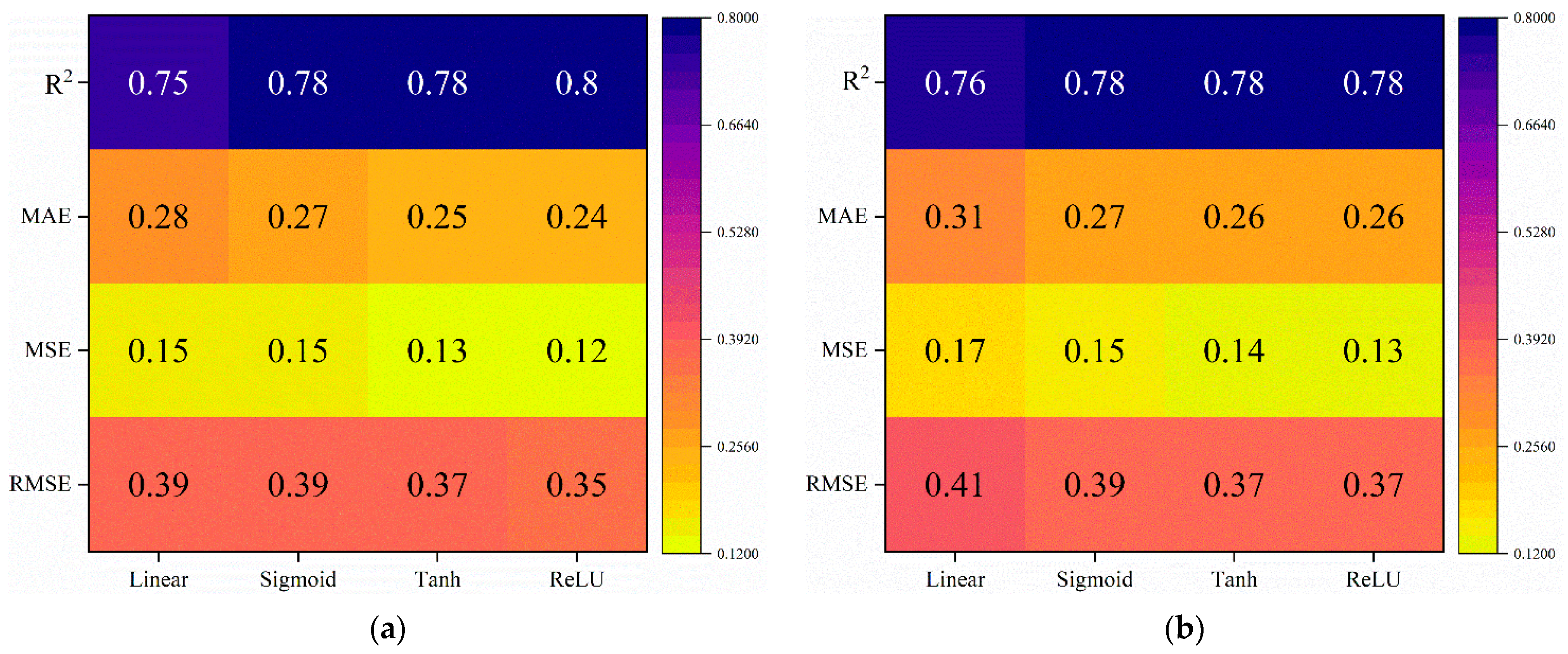
5.2. Predictive Capability Evaluation of Activation Functions
Activation functions can compensate for the shortcomings of the ANN model in learning and understanding very complex and nonlinear functions of underground structures. As described in Section 2, an appropriate activation function can accelerate the calculation speed and convergence speed of the ANN model, reduce the dependence between model parameters, and effectively alleviate the overfitting phenomenon. The linear function, Sigmoid function, Tanh function, and ReLU function are studied and the corresponding coefficients of the MSE, RMSE, MAE, and R2 are illustrated in Figure 12. It can be concluded that the predicted values of the Sigmoid function, Tanh function, and ReLU function in the ANN models are correlated with the training database because they have a more significant correlation coefficient than the linear function. In addition, the smallest MAE, MSE, and RMSE of 0.24, 0.12, and 0.35 are attributed to the ReLU function, which means that this function is the most efficient activation function for the training database. For the testing database, the MSE of the ReLU function has the lowest dispersion with regard to the other activation functions, and the ranking of the ANN models is ReLU > Tanh > Sigmoid > linear function, as displayed in Figure 12b. Compared with the linear function, the correlation coefficients (R2 = 0.78) of the Tanh activation function and Sigmoid activation function are obviously more significant than 0.76. In addition, the error of the PSDM model established by traditional linear analysis may be large, which will distort the vulnerability assessment results for the CFHTs.
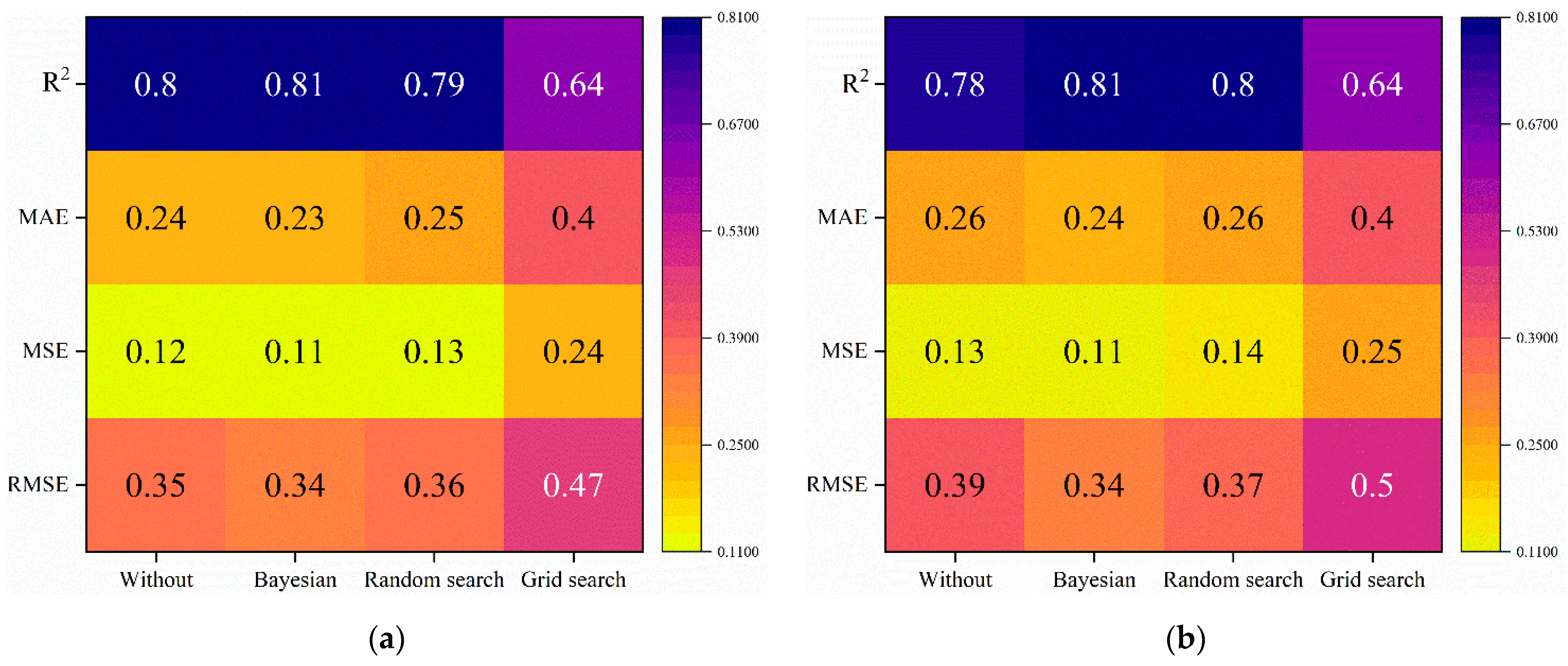
5.3. Predictive Capability Evaluation of Optimization Algorithm
A reasonable optimization function can significantly improve the predictive ability and accuracy of the neural network algorithm model while reducing the value of the MSE. Figure 13 compares the coefficients of MSE, RMSE, MAE, and R2 in the training database and testing database using the Bayesian optimization algorithm, random search optimization algorithm, and grid search optimization algorithm and without an optimization algorithm. As expected, the largest and smallest coefficients occur with the Bayesian optimization algorithm. The corresponding values are 0.11, 0.34, 0.23, and 0.81 for the training database, as shown in Figure 13a. Conversely, the grid search optimization algorithm is not suitable for the construction of ANN models. The main reason is that the predicted value is not closely related to the structural EDP and the error is significantly larger than for the other optimization algorithms. Moreover, the applicability of the grid optimization algorithm is lower than when not using an optimization algorithm, both in the training database and testing database (see Figure 13). Thus, not all optimization algorithms can improve the predictive ability of ANN models, especially for a highly nonlinear database. Based on the present results, in the next section, the hyper-parameters selected for the ANN models are as follows: 10 neuros, two hidden layers, the ReLU activation function, and the Bayesian optimization algorithm. These are applied to predict the structural response.
6. Analysis Results and Discussion
6.1. Investigation of the Effect of Seismology Features on Response Uncertainties
Selecting the seismology features of the input layers is a critical step in building ANN models, mainly because the seismology features are closely related to the structural responses. To reduce the error associated with the ANN model, six different types of seismology characteristics are studied to select the appropriate neurons for the input layers. Table 3 reports the values of RMSE, MSE, MAE, and R2 of the ANN models for the training and testing datasets under different seismology features. The trends of the RMSE, MSE, MAE, and R2 in Table 3 are significantly different among the examined cases. The smallest RMSE, MSE, and MAE of Case 4 for the training database and testing database compared to other examined cases indicate that the discreteness of the predicted database for the amplitude type is much higher than for seismology features such as PGA, PGV, and PGD. It is also found that the values of R2 for Cases 1–3 and Case 5 in Table 3 are smaller than those calculated for Case 4. Moreover, it can be found from Table 3 that there is a lower correlation coefficient regarding the integral and frequency content of seismology features compared with the other examined cases. Simultaneously, the coefficients of RMSE, MSE, and MAE for Case 5 and Case 6 are more significant than those for the other examined cases, which means that the predicted database of the corresponding ANN models is not suitable for the subsequent vulnerability analysis. The results also show that each set of information tends to compensate for its limitations, limiting the application of the seismic performance assessment.
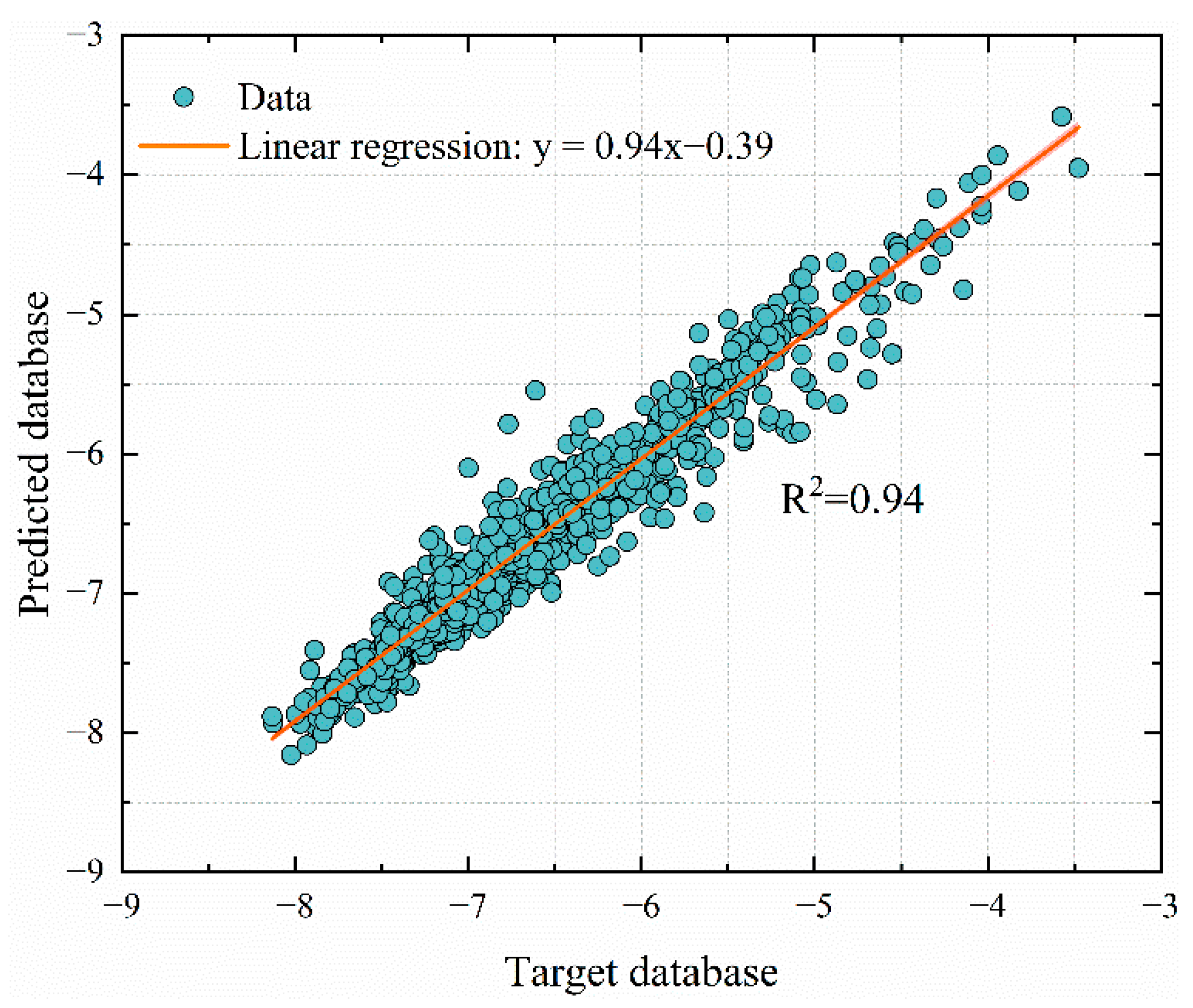
6.2. The Feasibility of the Predicted Database by the Proposed ANN Model
The 1080 numerical results calculated by FE simulation are compared with the predicted database of the ANN model in the logarithmic space, as shown in Figure 14. With regard to the correlation from the simple linear regression, the values predicted by the ANN model are strongly associated with the calculated values of the FE dynamic analysis of the CFHT, as shown in Figure 14. In general, the higher the correlation coefficient between the predicted database and the simulation database, the better the ability of the ANN model to predict the structural response. Meanwhile, the statistical distribution characteristics of the structural response for the ANN model and simulation results are studied, as shown in Figure 15. In this figure, the purple rectangle represents the relative frequency of SDIs, and the orange curve is the final result of the Gaussian function fitting. It can be found that the distribution of the predicted EDP of the CFHT under the ANN model has a slight difference from the target database. The difference in the corresponding mean value and the standard deviation is 0.01, which means that the proposed ANN model can predict the nonlinear behavior of CFHTs during low-strength and high-strength seismic events.
To further demonstrate the application of the ANN model in seismic performance assessment, the PSDM of the traditional seismic vulnerability analysis is utilized to derive the statistical seismic IM–demand measure relation, as shown in Figure 16. It can be seen from Figure 16a that the correlation coefficient of the PSDM from the FE simulation data is 0.86, showing a better correlation between the targeted database and PGV. Mathematically, the higher the correlation coefficient between the PGV and EDP, the better the ability of the PGV to explain the EDP and to decrease the uncertainty induced by seismic events. For the predicted database, the correlation coefficients (R2 = 0.90) of the PSDM between the PGV and EDP are significantly larger than that of the PGV and FE simulation EDP. In other words, the ANN model has sufficient potential and reliability to bridge the gap between the PGV and EDPs for structural performance assessment. Moreover, the efficiency () of the PSDM related to the PGV and EDP is displayed in Figure 16b. With the consideration of the ANN model and FE simulation, it can be found that the PSDM developed by the predicted database presents better efficiency, , than the target database, . Obviously, the ANN model has the potential to reduce the computational costs and develop appropriate PSDMs for the CFHT.
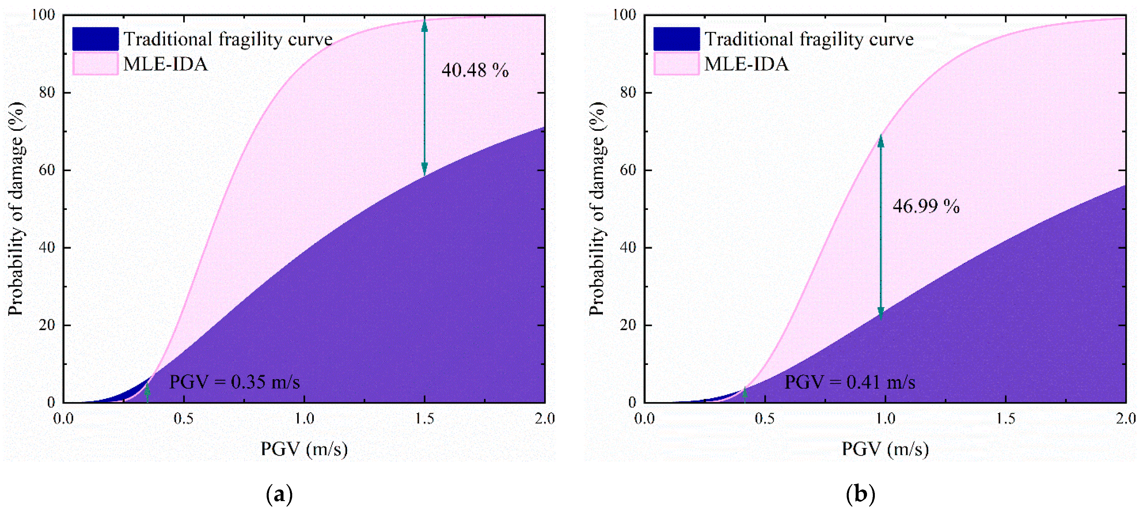
6.3. Seismic Fragility Analysis Using the Probabilistic ANN Model
A comprehensive fragility curve of CFHTs produced by the probabilistic ANN model is presented according to the MLE-IDA methodology and traditional fragility analysis, as displayed in Figure 17. Under slight/moderate damage, the exceedance probability of the MLE-IDA fragility curve of the CFHT is equal to 98.66% at , which exceeds the value of the traidiotnal fragility curve by approximately 40.48%. Furthermore, it can be found that only when the PGV exceeds 0.35 m/s does the probability of damage to the MLE-IDA exceed that of the traditional fragility curve. However, the difference between the MLE-IDA and the traditional approach is very small. Specifically, the traditional approach to evaluating the damage probability in the slight/moderate DS of CFHTs is generally poorer than the MLE-IDA method. Similarly, the exceedance probability of the CFHT based on the MLE-IDA method is also significantly larger than that of the traditional method when the seismic intensity exceeds 0.41 m/s. For example, the exceedance probability of the CFHT under the MLE-IDA and traditional method is approximately 31.12% and 84.74%, for , respectively. As the PGV increases, the size of the difference between the MLE-IDA and traditional method also increases gradually. It is worth emphasizing that the above phenomenon induced by the PSDM of underground structures tends to overestimate the EDP under extremely seismic excitation [49].
7. Final Remarks
The work presented herein explored the application of a deep learning methodology to predict the EDPs and generate fragility curves. For this purpose, the regression algorithms of artificial neural networks (ANNs) were investigated by tests to identify the optimal hyper-parameters to predict the structural response. The main seismology characteristics were also considered in different cases, and multivariate earthquake IM features can be integrated into one seismic IM feature through dimensionality reduction. Then, a three-dimensional (3D) numerical cross-fault hydraulic tunnel (CFHT) considering the nonlinear interaction system was chosen as a typical structure to conduct the dynamic time history analysis. Given the input training database regarding the integrated IM and the structural response of the finite element model, the proposed ANN method helps to produce different prediction models. Subsequently, the statistical parameters of the structural responses in the prediction models were compared to test the ANN methodology, while the ANN-based fragility curves of IDA were constructed via the maximum likelihood estimation (MLE) method. From the attained results, the following conclusions can be obtained.
- (1)
- Compared with the hyper-parameters in terms of the mean square error, root mean square error, mean absolute error, and correlation based on the training database and testing database, it was found that two hidden layers and ten neurons are most suitable parameters for the ANN model. Meanwhile, it was demonstrated that the Bayesian optimization algorithm has higher predictive power for structural responses than other examined optimization algorithms. Furthermore, the direct use of the ANN model is not recommended to predict the structural response for the CFHT since different hyper-parameters have various abilities to change the predicted capacity of the model.
- (2)
- The predicted database of the integrated peak-value-type IMs of the input layers is more reliable than the scalar-valued IMs according to the examined methods. For the studied case, it was also confirmed that the amplitude type of seismology characteristics predicted by the ANN model has the highest prediction capacity compared with the other examined seismology features. On the other hand, the integral type of seismology characteristics is not suitable for the input layers of the ANN model to predict the structural response.
- (3)
- Only a slight difference was observed from the PSDM between the predicted EDPs and the calculated value of the CFHT, indicating that it is a reliable tool for the estimation of the seismic performance of CFHTs. Meanwhile, the ANN model is most suitable for the fragility analysis of the CFHTs because it can improve the computational efficiency and overcome the normally distributed assumption. For the seismic fragility curves, the traditional fragility analysis method may underestimate the probability of damage to CFHTs compared with MLE-IDA.
In regard to this study, some limitations should be noted. For instance, the nonlinear dynamic plastic model was assumed to be the Drucker and Prager model, which may lead to dangerously biased conclusions for the tunnel under dynamic conditions. In addition, only the incoming angles of the vertical SV waves were utilized to describe the input of the earthquake load. Moreover, there is still a great deal of work that needs to be done in order to improve the proposed strategy. Different seismology features of earthquake records and multiple evaluation indicators of the structural response should be employed in order to more efficiently express the probability of damage of structures. The corrosion mechanism of the concrete lining induced by complex engineering environments should be further discussed in future studies. Meanwhile, the use of different metamodels, power or nonlinear regression models, statistical approaches, and probabilistic seismic hazard analysis can be considered to improve the prediction accuracy of the deep learning model.
Author Contributions
Conceptualization, W.C.; Methodology, B.S.; Software, P.W. All authors have read and agreed to the published version of the manuscript.
Funding
Financial support from the State Key Laboratory of Hydraulic Engineering Intelligent Construction and Operation of Tianjin Unviersity under the grant of HESS-2213 is gratefully acknowledged.
Institutional Review Board Statement
Not applicable.
Informed Consent Statement
Not applicable.
Data Availability Statement
The data presented in this study are available on request from the corresponding author. The data are not publicly available due to privacy issues.
Conflicts of Interest
The authors declare no conflict of interest.
References
- Hashash, Y.M.A.; Hook, J.J.; Schmidt, B.; Yao, J.I.C. Seismic design and analysis of underground structures. Tunn. Undergr. Sp. Technol. 2001, 16, 247–293. [Google Scholar] [CrossRef]
- Li, T. Damage to mountain tunnels related to the Wenchuan earthquake and some suggestions for aseismic tunnel construction. Bull. Eng. Geol. Environ. 2012, 71, 297–308. [Google Scholar] [CrossRef]
- Shen, Y.; Gao, B.; Yang, X.; Tao, S. Seismic damage mechanism and dynamic deformation characteristic analysis of mountain tunnel after Wenchuan earthquake. Eng. Geol. 2014, 180, 85–98. [Google Scholar] [CrossRef]
- Wang, X.; Chen, J.; Xiao, M. Seismic damage assessment and mechanism analysis of underground powerhouse of the Yingxiuwan Hydropower Station under the Wenchuan earthquake. Soil Dyn. Earthq. Eng. 2018, 113, 112–123. [Google Scholar] [CrossRef]
- Wang, Z.Z.; Zhang, Z. Seismic damage classification and risk assessment of mountain tunnels with a validation for the 2008 Wenchuan earthquake. Soil Dyn. Earthq. Eng. 2013, 45, 45–55. [Google Scholar] [CrossRef]
- Yu, H.; Chen, J.; Bobet, A.; Yuan, Y. Damage observation and assessment of the Longxi tunnel during the Wenchuan earthquake. Tunn. Undergr. Sp. Technol. 2016, 54, 102–116. [Google Scholar] [CrossRef]
- Bazzurro, P.; Cornell, C.A.; Shome, N.; Carballo, J.E. Three proposals for characterizing MDOF nonlinear seismic response. J. Struct. Eng. 1998, 124, 1281–1289. [Google Scholar] [CrossRef]
- Cornell, C.A.; Jalayer, F.; Hamburger, R.O.; Foutch, D.A. Probabilistic basis for 2000 SAC federal emergency management agency steel moment frame guidelines. J. Struct. Eng. 2002, 128, 526–533. [Google Scholar] [CrossRef]
- Baker, J.W. Efficient analytical fragility function fitting using dynamic structural analysis. Earthq. Spectra 2015, 31, 579–599. [Google Scholar] [CrossRef]
- Baker, J.W. Quantitative classification of near-fault ground motions using wavelet analysis. Bull. Seismol. Soc. Am. 2007, 97, 1486–1501. [Google Scholar] [CrossRef]
- Kim, T.; Song, J.; Kwon, O.-S. Probabilistic evaluation of seismic responses using deep learning method. Struct. Saf. 2020, 84, 101913. [Google Scholar] [CrossRef]
- Kiani, J.; Camp, C.; Pezeshk, S. On the application of machine learning techniques to derive seismic fragility curves. Comput. Struct. 2019, 218, 108–122. [Google Scholar] [CrossRef]
- Wang, Z.; Pedroni, N.; Zentner, I.; Zio, E. Seismic fragility analysis with artificial neural networks: Application to nuclear power plant equipment. Eng. Struct. 2018, 162, 213–225. [Google Scholar] [CrossRef]
- Huang, Z.; Argyroudis, S.A.; Pitilakis, K.; Zhang, D.; Tsinidis, G. Fragility assessment of tunnels in soft soils using artificial neural networks. Undergr. Sp. 2022, 7, 242–253. [Google Scholar] [CrossRef]
- Noureldin, M.; Ali, A.; Memon, S.; Kim, J. Fragility-based framework for optimal damper placement in low-rise moment-frame buildings using machine learning and genetic algorithm. J. Build. Eng. 2022, 54, 104641. [Google Scholar] [CrossRef]
- Liu, C.; Macedo, J. Machine learning-based models for estimating seismically-induced slope displacements in subduction earthquake zones. Soil Dyn. Earthq. Eng. 2022, 160, 107323. [Google Scholar] [CrossRef]
- Li, Z.; Wu, Z.; Lu, X.; Zhou, J.; Chen, J.; Liu, L.; Pei, L. Efficient seismic risk analysis of gravity dams via screening of intensity measures and simulated non-parametric fragility curves. Soil Dyn. Earthq. Eng. 2022, 152, 107040. [Google Scholar] [CrossRef]
- Jingchi, Y.U.; Aiyun, J.I.N.; Jianwen, P.A.N.; Jinting, W.; Chuhan, Z. GA-BP artificial neural networks for predicting the seismic response of arch dams. J. Tsinghua Univ. (Sci. Technol.) 2022, 62, 1321–1329. [Google Scholar]
- Dang-Vu, H.; Nguyen, Q.D.; Chung, T.; Shin, J.; Lee, K. Frequency-based Data-driven Surrogate Model for Efficient Prediction of Irregular Structure’s Seismic Responses. J. Earthq. Eng. 2022, 26, 7319–7336. [Google Scholar] [CrossRef]
- Ghasemi, A.; Stephens, M.T. Building clustering for regional seismic response and damage analysis. Earthq. Spectra 2022, 38, 2941–2969. [Google Scholar] [CrossRef]
- Işık, E.; Ademović, N.; Harirchian, E.; Avcil, F.; Büyüksaraç, A.; Hadzima-Nyarko, M.; Akif Bülbül, M.; Işık, M.F.; Antep, B. Determination of Natural Fundamental Period of Minarets by Using Artificial Neural Network and Assess the Impact of Different Materials on Their Seismic Vulnerability. Appl. Sci. 2023, 13, 809. [Google Scholar] [CrossRef]
- Jena, R.; Naik, S.P.; Pradhan, B.; Beydoun, G.; Park, H.-J.; Alamri, A. Earthquake vulnerability assessment for the Indian subcontinent using the Long Short-Term Memory model (LSTM). Int. J. Disaster Risk Reduct. 2021, 66, 102642. [Google Scholar] [CrossRef]
- Kazemi, F.; Asgarkhani, N.; Jankowski, R. Machine learning-based seismic fragility and seismic vulnerability assessment of reinforced concrete structures. Soil Dyn. Earthq. Eng. 2023, 166, 107761. [Google Scholar] [CrossRef]
- Soleimani, F.; Liu, X. Artificial neural network application in predicting probabilistic seismic demands of bridge components. Earthq. Eng. Struct. Dyn. 2022, 51, 612–629. [Google Scholar] [CrossRef]
- Urlainis, A.; Shohet, I.M. Development of Exclusive Seismic Fragility Curves for Critical Infrastructure: An Oil Pumping Station Case Study. Buildings 2022, 12, 842. [Google Scholar] [CrossRef]
- Urlainis, A.; Shohet, I.M. Seismic Risk Mitigation and Management for Critical Infrastructures Using an RMIR Indicator. Buildings 2022, 12, 1748. [Google Scholar] [CrossRef]
- Xu, Z.; Chen, J.; Shen, J.; Xiang, M. Regional-scale nonlinear structural seismic response prediction by neural network. Eng. Fail. Anal. 2023, 154, 107707. [Google Scholar] [CrossRef]
- Morgenroth, J.; Khan, U.T.; Perras, M.A. An overview of opportunities for machine learning methods in underground rock engineering design. Geosciences 2019, 9, 504. [Google Scholar] [CrossRef]
- Chimunhu, P.; Topal, E.; Ajak, A.D.; Asad, W. A review of machine learning applications for underground mine planning and scheduling. Resour. Policy 2022, 77, 102693. [Google Scholar] [CrossRef]
- Li, N.; Nguyen, H.; Rostami, J.; Zhang, W.; Bui, X.-N.; Pradhan, B. Predicting rock displacement in underground mines using improved machine learning-based models. Measurement 2022, 188, 110552. [Google Scholar] [CrossRef]
- Mahmoodzadeh, A.; Mohammadi, M.; Ibrahim, H.H.; Noori, K.M.G.; Abdulhamid, S.N.; Ali, H.F.H. Forecasting sidewall displacement of underground caverns using machine learning techniques. Autom. Constr. 2021, 123, 103530. [Google Scholar] [CrossRef]
- Pu, Y.; Apel, D.B.; Hall, R. Using machine learning approach for microseismic events recognition in underground excavations: Comparison of ten frequently-used models. Eng. Geol. 2020, 268, 105519. [Google Scholar] [CrossRef]
- Liu, Z.; Li, S.; Guo, A.; Li, H. Comprehensive functional resilience assessment methodology for bridge networks using data-driven fragility models. Soil Dyn. Earthq. Eng. 2022, 159, 107326. [Google Scholar] [CrossRef]
- Ellingwood, B. Validation studies of seismic PRAs. Nucl. Eng. Des. 1990, 123, 189–196. [Google Scholar] [CrossRef]
- Vasavada, M.; Patel, V.R. Development of Fragility Curves for RC Buildings using HAZUS method. Int. Res. J. Eng. Technol. 2016, 3. [Google Scholar] [CrossRef]
- Goulet, J.-A. Probabilistic Machine Learning for Civil Engineers; MIT Press: Cambridge, MA, USA, 2020; ISBN 0262358018. [Google Scholar]
- Segura, R.; Padgett, J.E.; Paultre, P. Metamodel-based seismic fragility analysis of concrete gravity dams. J. Struct. Eng. 2020, 146, 04020121. [Google Scholar] [CrossRef]
- Kuhlemeyer, R.L.; Lysmer, J. Finite element method accuracy for wave propagation problems. J. Soil Mech. Found. Div 1973, 99, 421–427. [Google Scholar] [CrossRef]
- Drucker, D.C.; Prager, W. Soil mechanics and plastic analysis or limit design. Q. Appl. Math. 1952, 10, 157–165. [Google Scholar] [CrossRef]
- Sun, B.; Liu, W.; Deng, M.; Zhang, S.; Wang, C.; Guo, J.; Wang, J.; Wang, J. Compound intensity measures for improved seismic performance assessment in cross-fault hydraulic tunnels using partial least-squares methodology. Tunn. Undergr. Sp. Technol. 2023, 132, 104890. [Google Scholar] [CrossRef]
- Hatzigeorgiou, G.D.; Beskos, D.E. Soil–structure interaction effects on seismic inelastic analysis of 3-D tunnels. Soil Dyn. Earthq. Eng. 2010, 30, 851–861. [Google Scholar] [CrossRef]
- Sun, B.; Deng, M.; Zhang, S.; Wang, C.; Cui, W.; Li, Q.; Xu, J.; Zhao, X.; Yan, H. Optimal selection of scalar and vector-valued intensity measures for improved fragility analysis in cross-fault hydraulic tunnels. Tunn. Undergr. Sp. Technol. 2023, 132, 104857. [Google Scholar] [CrossRef]
- Dobry, R.; Idriss, I.M.; Ng, E. Duration characteristics of horizontal components of strong-motion earthquake records. Bull. Seismol. Soc. Am. 1978, 68, 1487–1520. [Google Scholar]
- Kramer, S.L. Geotechnical Earthquake Engineering; Pearson Education India: Noida, India, 1996; ISBN 8131707180. [Google Scholar]
- Arias, A. Measure of Earthquake Intensity; Massachusetts Institute of Technology, Cambridge University of Chile: Santiago, Chile, 1970. [Google Scholar]
- Von Thun, J.L. Earthquake ground motions for design and analysis of dams. Earthq. Eng. Soil Dyn. II-Recent Adv. Ground-Motion Eval. 1988, 18, 227–239. [Google Scholar]
- Liu, J.B.; Du, Y.X.; Du, X. 3D viscous-spring artificial boundary in time domain. Earthq. Eng. Eng. Vib. 2006, 5, 93–102. [Google Scholar] [CrossRef]
- Andreotti, G.; Lai, C.G. Use of fragility curves to assess the seismic vulnerability in the risk analysis of mountain tunnels. Tunn. Undergr. Sp. Technol. 2019, 91, 103008. [Google Scholar] [CrossRef]
- Huang, P.; Chen, Z. Fragility analysis for subway station using artificial neural network. J. Earthq. Eng. 2021, 1–21. [Google Scholar] [CrossRef]
Figure 1.
Typical neuron structure in the human body.

Figure 2.
A classical multilayer feed-forward backpropagation network of ANNs.

Figure 3.
Explanation of the workflow of the ANN model.

Figure 4.
Framework of seismic vulnerability analysis for CFHTs.

Figure 5.
Schematic of the FE model of CFHT.

Figure 6.
Stress–strain curve of the concrete lining. (a) Damage factor and compressive stress–strain; (b) Damage factor and tensile stress–strain [40].
Figure 6.
Stress–strain curve of the concrete lining. (a) Damage factor and compressive stress–strain; (b) Damage factor and tensile stress–strain [40].

Figure 7.
The flowchart of the static and dynamic analysis for CFHT.

Figure 8.
The earthquake magnitude and fault distance of the selected GM records.

Figure 9.
The spectral acceleration of the selected GM records.

Figure 10.
Comparing the coefficients obtained from RMSE, MSE, MAE, and R2 for the different numbers of hidden layers: (a) target database and (b) predicted database.
Figure 10.
Comparing the coefficients obtained from RMSE, MSE, MAE, and R2 for the different numbers of hidden layers: (a) target database and (b) predicted database.

Figure 11.
Comparing the coefficients obtained from RMSE, MSE, MAE, and R2 for the different numbers of neurons: (a) target database and (b) predicted database.
Figure 11.
Comparing the coefficients obtained from RMSE, MSE, MAE, and R2 for the different numbers of neurons: (a) target database and (b) predicted database.

Figure 12.
Comparing the coefficients obtained from RMSE, MSE, MAE, and R2 for the different activation functions: (a) target database and (b) predicted database.
Figure 12.
Comparing the coefficients obtained from RMSE, MSE, MAE, and R2 for the different activation functions: (a) target database and (b) predicted database.

Figure 13.
Comparing the coefficients obtained from RMSE, MSE, MAE, and R2 for the different optimization algorithms: (a) target database and (b) predicted database.
Figure 13.
Comparing the coefficients obtained from RMSE, MSE, MAE, and R2 for the different optimization algorithms: (a) target database and (b) predicted database.

Figure 14.
Comparison of the correlation between the predicted database and target database.

Figure 15.
The statistical distribution characteristics of the structural response for the ANN model and simulation results: (a) target database and (b) predicted database.
Figure 15.
The statistical distribution characteristics of the structural response for the ANN model and simulation results: (a) target database and (b) predicted database.

Figure 16.
The statistical distribution characteristics of the structural response for the ANN model and simulation results: (a) target database and (b) predicted database.
Figure 16.
The statistical distribution characteristics of the structural response for the ANN model and simulation results: (a) target database and (b) predicted database.

Figure 17.
Comparison of fragility curves of the CFHT between the GP-PCA and numerical results: (a) slight/moderate damage and (b) severe damage.
Figure 17.
Comparison of fragility curves of the CFHT between the GP-PCA and numerical results: (a) slight/moderate damage and (b) severe damage.


Table 1.
The IMs considered in this investigation.
| Description | Symbol | Definition | Unit | Reference |
|---|---|---|---|---|
| Peak Ground Acceleration | PGA | g | - | |
| Peak Ground Velocity | PGV | m/s | - | |
| Acceleration Root-Mean-Square | Arms | g | [43] | |
| Velocity RMS | Vrms | m | [44] | |
| Arias Intensity | IA | m/s | [45] | |
| Acceleration Spectrum Intensity | ASI | m*s | [46] | |
| Velocity Spectrum Intensity | VSI | m | [46] |
Table 2.
Definitions of the DS, damage level, and damage measures [48].
Table 2.
Definitions of the DS, damage level, and damage measures [48].
| Damage State | Damage Level | Damage Measures | |
|---|---|---|---|
| Drift Ratio | Log Std | ||
| DS0 | No damage | - | - |
| DS1 | Slight/moderate damage | ||
| DS2 | Extensive damage | ||
Table 3.
Comparison of RMSE, MSE, MAE, and R2 for the training and testing datasets under different seismology features.
Table 3.
Comparison of RMSE, MSE, MAE, and R2 for the training and testing datasets under different seismology features.
| Case | Seismology Features | Database | RMSE | MSE | MAE | R2 |
|---|---|---|---|---|---|---|
| Case 1 | PGV | Train | 0.34 | 0.11 | 0.23 | 0.81 |
| Test | 0.34 | 0.11 | 0.24 | 0.81 | ||
| Case 2 | PGV and Vrms | Train | 0.32 | 0.10 | 0.22 | 0.84 |
| Test | 0.33 | 0.11 | 0.24 | 0.82 | ||
| Case 3 | Peak values (PGA, PGV, PGD) | Train | 0.29 | 0.09 | 0.21 | 0.86 |
| Test | 0.30 | 0.09 | 0.22 | 0.86 | ||
| Case 4 | Amplitude | Train | 0.24 | 0.06 | 0.17 | 0.91 |
| Test | 0.22 | 0.05 | 0.16 | 0.92 | ||
| Case 5 | Integral | Train | 0.47 | 0.22 | 0.37 | 0.66 |
| Test | 0.46 | 0.21 | 0.36 | 0.65 | ||
| Case 6 | Frequency content | Train | 0.37 | 0.13 | 0.27 | 0.80 |
| Test | 0.33 | 0.11 | 0.24 | 0.79 |
Disclaimer/Publisher’s Note: The statements, opinions and data contained in all publications are solely those of the individual author(s) and contributor(s) and not of MDPI and/or the editor(s). MDPI and/or the editor(s) disclaim responsibility for any injury to people or property resulting from any ideas, methods, instructions or products referred to in the content. |
© 2023 by the authors. Licensee MDPI, Basel, Switzerland. This article is an open access article distributed under the terms and conditions of the Creative Commons Attribution (CC BY) license (https://creativecommons.org/licenses/by/4.0/).
Share and Cite
MDPI and ACS Style
Cao, W.; Sun, B.; Wang, P. Application of a Deep Learning Method to the Seismic Vulnerability Analysis of Cross-Fault Hydraulic Tunnels Based on MLE-IDA. Appl. Sci. 2023, 13, 13232. https://doi.org/10.3390/app132413232
AMA Style
Cao W, Sun B, Wang P. Application of a Deep Learning Method to the Seismic Vulnerability Analysis of Cross-Fault Hydraulic Tunnels Based on MLE-IDA. Applied Sciences. 2023; 13(24):13232. https://doi.org/10.3390/app132413232
Chicago/Turabian StyleCao, Wenyu, Benbo Sun, and Pengxiao Wang. 2023. "Application of a Deep Learning Method to the Seismic Vulnerability Analysis of Cross-Fault Hydraulic Tunnels Based on MLE-IDA" Applied Sciences 13, no. 24: 13232. https://doi.org/10.3390/app132413232
Note that from the first issue of 2016, this journal uses article numbers instead of page numbers. See further details here.