
A Residual Voltage Data-Driven Prediction Method for Voltage Sag Based on Data Fusion
by
 ,
,
Chen Zheng
1 ,
,
Shuangyin Dai
1,
Bo Zhang
1,
Qionglin Li
1,
Shuming Liu
1,
Yuzheng Tang
1,
Yi Wang
1,
Yifan Wu
2 and
Yi Zhang
2,* 1
Electric Power Research Institute of State Grid Henan Electric Power Company, Zhengzhou 450052, China
2
College of Electrical Engineering and Automation, Fuzhou University, Fuzhou 350100, China
*
Author to whom correspondence should be addressed.
Symmetry 2022, 14(6), 1272; https://doi.org/10.3390/sym14061272
Submission received: 27 May 2022
/
Revised: 11 June 2022
/
Accepted: 15 June 2022
/
Published: 20 June 2022
(This article belongs to the Special Issue Advanced Technologies in Power Quality and Power Disturbance Data Application)
Abstract
:Voltage sag is the most serious power quality problem in the three-phase symmetrical power system. The influence of multiple factors on the voltage sag level and low computational efficiency also pose challenges to the prediction of residual voltage amplitude of voltage sag. This paper proposes a voltage sag amplitude prediction method based on data fusion. First, the multi-dimensional factors that influence voltage sag residual voltage are analyzed. Second, these factors are used as input, and a model for predicting voltage sag residual voltage based on data fusion is constructed. Last, the model is trained and debugged to enable it to predict the voltage sag residual voltage. The accuracy and feasibility of the method are verified by using the actual power grid data from East China.
1. Introduction
Voltage sag is an inevitable short-term disturbance phenomenon that appears during power system operation, and it has become the most serious power quality problem. Voltage sag affects voltage quality and causes considerable economic losses [1,2]. The influencing degree of voltage sag mainly depends on the residual voltage amplitude. Accurate prediction of the residual voltage of the voltage sag can help in clearly understanding the impact of voltage dip on equipment and users. Furthermore, it can provide the basis for users to prevent or control voltage sag, which is very important for reducing the impact of voltage sag [3].
In refs. [4,5], the authors used the Monte Carlo method to express the uncertainty of fault occurrence, including fault type, fault location, etc., and subsequently predicted the probability distribution of voltage sag residual voltage amplitude. The Monte Carlo method cannot consider the influence of the actual environment on the prediction.The authors in [6] pointed out that the influences of generator scheduling and time-varying failure rate on the random prediction of voltage sag should be considered during the voltage sag prediction process. In ref. [7], the authors proposed an online algorithm for residual voltage amplitude prediction based on the harmonic footprint and constructed a general prediction function suitable for all voltage disturbances.
A few methods use monitoring data to predict the voltage sag index. In ref. [8], the authors used the monitoring data to analyze and discuss the randomness of voltage sag. Furthermore, the authors described the voltage sag as a random process and predicted a sag event. In ref. [9], the authors used measured data to predict the voltage sag frequency index of non-monitoring points. The authors in [10] used homologous aggregation and fuzzy c-means theory to reduce the redundancy of the measured data and predict the residual voltage. The aforementioned prediction methods based on monitoring data need long monitoring times and low amounts of monitoring data, which lead to poor prediction accuracies.
This paper proposes a data-driven method for voltage sag residual voltage prediction based on data fusion. The original contributions of this study are summarized as follows:
- (1)
- This paper comprehensively considers the factors influencing the grid and user sides in order to predict voltage sag residual voltage. The corresponding input parameters are selected from different kinds of data and the factors that influence the residual voltage are considered more comprehensively than the Monte Carlo-based method.
- (2)
- This paper builds a prediction method based on data fusion to predict the residual voltage. The amount of data is increased through data fusion, and the problems of low prediction accuracy and low amount of available monitoring data are improved.
- (3)
- This paper presents a residual voltage prediction method for voltage sag based on data fusion, which can be integrated into power-quality-monitoring systems and used for the prevention, evaluation, and treatment of voltage sag. This method can provide users with residual voltage information and help them avoid voltage sag and formulate reasonable voltage sag prevention or treatment measures. The accuracy and efficiency of the method are verified using actual data, which gives it a strong engineering application value.
The remainder of this paper is organized as follows. The data sources of voltage sag residual voltage are described in Section 1. The residual voltage prediction method based on the improved gradient descent method is presented in Section 2. Case studies and analyses based on real power system data are shown in Section 3. The paper is concluded in Section 4.
2. Factors and Data Sources of Voltage Sag Residual Voltage
2.1. Influencing Factors of Voltage Sag Residual Voltage
Motor startup and other factors can cause voltage sag; however, these types of voltage sag are often not serious and existing measures can effectively eliminate their impact [11]. The main cause of voltage sag is a power grid fault [12]. Therefore, this paper mainly considers the impact of power grid faults during the voltage sag residual voltage prediction process.
After a grid fault occurs, the residual voltages at different nodes have varying amplitudes under different grid operation modes, and the impacts on different nodes are also different. Therefore, the influence of grid operation mode should also be considered in the prediction of the residual voltage of voltage sag. In addition, voltage sags are closely related to users. Different users are affected differently depending on the types of sags transmitted to them. Therefore, the influence of the user side should be considered in the prediction of voltage sag residual voltage amplitude. In summary, voltage sag residual voltage is related to fault conditions, grid operation mode, and the influence of the user side. The above factors are considered as the factors influencing the voltage sag residual voltage and used for selecting relevant data for voltage sag residual voltage prediction.
2.2. Data Sources
Voltage sag data can be obtained by the Monte Carlo random fault simulation method as follows: First, the fault parameters, such as fault type, fault distance, fault line, etc., are used as random variables and the simulation calculation is carried out by the Monte Carlo method. Second, the sag level of each bus in the area is obtained. Last, the simulated data are obtained. The simulated data can reflect the influence of system operation mode and fault on residual voltage, but cannot directly reflect the influence of external factors such as weather.
When a voltage sag occurs in the power grid, the power quality monitoring system, energy management system, user power consumption information collection system, and other systems collect a large number of records. There are many kinds of data related to voltage sag, and the relationship between them is complicated. In this paper, the relevant factors affecting the voltage sag residual voltage are obtained from the above multi-source system. The monitoring data not only reflect the influence of system operation mode and power grid faults, but also reflect the influence of external environmental factors and user-side influence. However, the data require long-term monitoring and consist of a small number of samples.
In summary, for the voltage sag residual voltage prediction, the data attributes reflecting the factors that influence the voltage sag residual voltage are selected from the simulated and measured data. These factors are shown in Table A1 of Appendix A.
3. Voltage Sag Residual Voltage Prediction Method
3.1. Multiple Regression Model and Gradient Descent Method
Voltage sag residual voltage is affected by many factors. Therefore, this paper uses the multiple regression model to characterize the effects of various factors on voltage sag residual voltage. This model can be expressed as follows:
where y is the dependent variable, x1, x2, x3… denote the independent variables, and θ1, θ2, θ3… represent the regression coefficients corresponding to x1, x2, x3…, respectively.
The gradient descent method is a type of line search framework algorithm with negative gradient as the search direction [13]. In order to minimize the loss function, the optimization model parameters are obtained iteratively until convergence is attained, and the best-matching target task is obtained.
The basic calculation process is as follows: Solving the model parameters for the loss function H(x1, x2…) can transform it into an optimization problem of min H(x1, x2…). The calculation of the gradient g(x1, x2…) is shown in (2). It is straightforward to conclude that the negative gradient direction −∇H is the fastest direction of decrease of the loss function. The iterative format of the gradient descent method is given by (3). Equations (2) and (3) shown below are iteratively used to reduce the loss function and approach the minimum point, and the parameters of the optimization model can be obtained after convergence.
In (3), k is the number of iterations, sk is the kth iteration step size, and gk is the kth iteration gradient size.
3.2. Multiple Regression Model Based on Improved Gradient Descent Method
3.2.1. Model Parameters
In order to realize the voltage sag residual voltage prediction using data fusion, this paper constructs a multiple regression model based on the improved gradient descent method. This improvement requires the construction of multiple regression models for the two types of data. The simulated data model is represented by Ds = f(x), and the input parameter is the attribute name corresponding to the simulated data in Table A1, including the common part of the two types of data. The model of the measured data is represented by Dm = g(y), and the input parameter is the attribute name corresponding to the measured data in Table A1, including the common part of the two types of data. The output results of Ds and Dm are the residual voltage amplitudes, expressed by Vs and Vm, respectively.
As the duration of sag mainly depends on the setting value of the protection device [10], it is not predicted in this paper. It can be observed from Table A1 that there is a common input data attribute with a consistent description in the simulated and measured data. This part is represented by the set Ashared in this paper, and the corresponding regression coefficient is represented by θshared. The non-common part attributes of the two types of data are represented by As and Am, and the corresponding regression coefficients are represented by θs and θm, respectively. The subscripts s and m represent the simulated and measured data models, respectively. During the process of searching for the optimal model parameters using the improved gradient descent method, the loss functions Hs(x) and Hm(z) of the two models are given as
where n and h are the simulated and measured data sample capacities, respectively; xi and Vs(i) correspond to the input and output of the ith simulation data sample, respectively; and zj and Vm(j) correspond to the input and output of the jth measured data sample, respectively.
3.2.2. Model Update Strategy
This paper presents an improved gradient descent method. When the output of the two models is the residual voltage amplitude, the functions of Ashared in both Ds and Dm are identical. Therefore, considering the simulated and measured data as the source and target domains, respectively, the prior knowledge obtained by simulation in Ds is migrated to Dm for updating θshared. After completing the migration, the updated θshared is substituted back into the original model and the updated θs and θm are recalculated to complete the single-learning process. At this time, Dm not only reflects the role of the factors influencing the voltage sag residual voltage from the information point of view, but also reveals the impacts of relevant factors on the voltage sag residual voltage from the physical point of view. The model realizes physical–information integration through knowledge migration and improves its information space and learning performance.
The traditional gradient descent method uses a constant, sk, whose value is obtained through trial and error. This method has the following problems: (1) The learning degree of the model is different in different stages of training; and (2) It takes a certain amount of time to obtain the ideal value of sk by multiple attempts.
In view of the above problems, this paper considers improving the step update strategy of the model. The Armijo–Goldstein criterion is introduced into the step size update process. There are two formulas for the Armijo–Goldstein criterion, which can be expressed by (6) and (7). The value of sk satisfying (6) and (7) is called an acceptable step size factor. After the introduction of the Armijo–Goldstein criterion, sk can be automatically updated to an acceptable step size factor and the algorithm will have superlinear convergence.
In (6) and (7), f(x) is the objective function, dk is the search direction, gk is the gradient size, and ρ ∈ (0, 0.5) to ensure the superlinear convergence of the algorithm.
3.3. Overall Process
To summarize, the process of voltage sag residual voltage prediction based on data fusion is as follows:
- (1)
- Acquire the measured data that can reflect the factors influencing the residual voltage from the multi-source system. The simulated data are obtained by a random sag simulation calculation based on the Monte Carlo method.
- (2)
- Carry out data preprocessing on the simulated and measured data to adapt them to the model, and use the above data as the model input.
- (3)
- Build a multiple regression model based on the improved gradient descent method. During the iterative process of the gradient descent method, the model updates the model parameters and adaptively adjusts the step size based on knowledge transfer and the Armijo–Goldstein criterion until convergence is reached.
- (4)
- After the training is completed, the model learns the knowledge from the physical and information aspects and can predict the residual voltage amplitude.
Figure 1 shows the overall flow chart of the voltage sag residual voltage prediction method proposed in this paper.
4. Case Study
4.1. Data Source and Input
This paper selects 57 voltage sag measured data samples from January 2021 to December 2021 in a city in eastern China. The simulated data are obtained using Monte Carlo random simulations. The simulation calculation process is mainly realized by Bonnevillr Power Administration (BPA) [14], which is power system simulation software commonly used by power companies. The region selected for study has long been affected by voltage sags, and there are many industrial users that have a large proportion of sensitive equipment in the region, which is representative for this study.
4.2. Residual Voltage Prediction
4.2.1. Prediction Results
The simulated and measured data are obtained according to Table 1 and are subsequently preprocessed. In the measured data, 44 samples are randomly selected as the training set, and the remaining 13 samples are used as the test set. The simulation dataset for knowledge transfer consists of 5280 data points obtained from the BPA-based Monte Carlo random simulation calculation.
The model uses root-mean-square error (RMSE) and mean absolute error (MAE) as the evaluation metrics. A total of 44 measured training data points and 5280 simulated training data points are input into the model for training. After training, the RMSE of the model on the training set is 0.1678, the MAE is 0.1377, and the model is able to predict the residual voltage amplitude.
In (8) and (9), i is the number of samples, xi is the actual value, and xi′ is the predicted value.
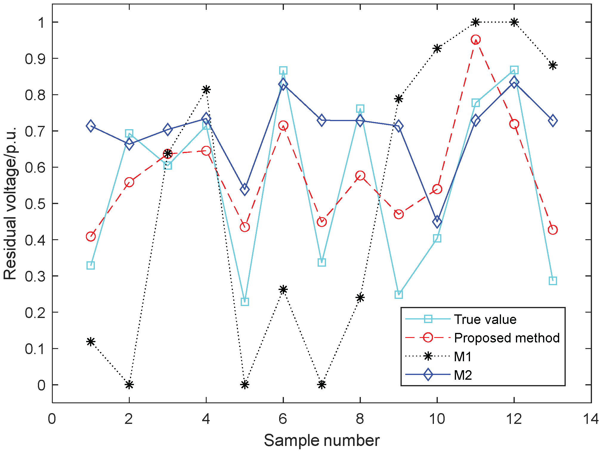
After the training, the method is tested on the test set data to verify its generalization ability. In order to evaluate the model performance, it is compared with the following methods: 1. The traditional gradient descent method [13], denoted as M1 here; and 2. A support vector machine [15] (SVM, rbf-kernel, ε = 0.0198), denoted as M2 here. Figure 2 shows the prediction results of each method, Table 1 shows the evaluation indices of each method and Table 2 shows the relative error between the predicted and actual values of each method.
The above results show that the RMSE and MAE of the proposed method are better than those of the other two methods. In addition, it can be observed from Table 2 that the relative prediction error of the method proposed in this paper is smaller than those of the other two methods. The method M1 has a large overall error and a large deviation from the error. At the same time, many output results of the method exceed the upper and lower limits of voltage amplitude and are limited by the threshold, indicating its poor convergence. Compared with M1, the output results obtained by the proposed method do not exceed the voltage amplitude limit. The convergence is improved and the error is considerably reduced.
The model structure of M2 is more complex than that of the proposed method. However, its evaluation metric is still slightly inferior compared to that of the proposed method. Although the complex model structure adopted in M2 can improve the error to a certain extent, the problem of small sample space still significantly impacts the model performance. The method proposed in this paper uses data fusion to improve the updating strategy of the model in M1 and enhance the data mining performance. Therefore, the proposed method achieves better results compared to M2.
4.2.2. Number of Iterations
Under the same convergence conditions, the numbers of iterations between the proposed method and M1 are compared in Table 3. The number of iterations of M2 is not compared here because of the different training methods.
Compared with M1, the number of iterations of the proposed method is significantly reduced. This is because the proposed method modifies the update mode of the model parameters and step size through data fusion. This modification improves the learning performance of the training process and accelerates the learning process. Thus, the number of iterations is significantly reduced.
In summary, the accuracy of this method is better than that of the other two methods, and the convergence performance is also significantly improved compared with M1. Therefore, in the actual power system, this method can predict the residual voltage of the possible voltage sag at fixed intervals by collecting relevant data. This prediction can help users to prevent and control the voltage sag and reduce economic losses.
5. Conclusions
In this paper, a voltage sag residual voltage data-driven prediction method based on data fusion was proposed and verified. The following conclusions were obtained:
- (1)
- This method analyzed the relevant factors affecting the residual voltage of voltage sag from multiple dimensions. The relevant influencing factors were selected as input in order to consider the factors influencing the residual voltage of voltage sag more comprehensively.
- (2)
- This method considered different data characteristics and realized the prediction of voltage sag residual voltage through data fusion. Consequently, the prediction accuracy and convergence rate were improved.
- (3)
- The method was convenient and practical, which was verified by examples. In the future, it can be used to predict the residual voltage of voltage sag and assist the analysis of voltage sag level and consequences.
Author Contributions
Conceptualization, Y.W. (Yifan Wu) and Y.Z.; methodology, Y.W. (Yifan Wu); software, Y.W. (Yifan Wu); validation, Y.W. (Yifan Wu), C.Z., and S.D.; formal analysis, C.Z. and B.Z.; investigation, C.Z. and S.L.; resources, Q.L. and Y.T.; writing—original draft preparation, Y.W. (Yifan Wu) and C.Z.; writing—review and editing, Y.W. (Yifan Wu) and Y.Z.; supervision, Y.W. (Yi Wang); project administration, C.Z. All authors have read and agreed to the published version of the manuscript.
Funding
This research is supported by the science and technology project of the headquarters of the State Grid Corporation of China (Key technologies and applications of digital mirroring for analysis and treatment of voltage sags in distribution networks, 5400-202124153A-0-0-00).
Conflicts of Interest
The authors declare no conflict of interest.
Abbreviations
| BPA | Bonnevillr Power Administration |
| RMSE | Root-mean-square error |
| MAE | Mean absolute error |
| SVM | Support vector machine |
Nomenclature
The subscript ‘s’ represents the simulation data model and the subscript ‘m’ represents the measured data model.
| Ds | Simulated data model |
| Dm | Measured data model |
| As | Unique parameters of simulated data model |
| Am | Unique parameters of measured data model |
| Ashared | Common parameters of simulated and measured data model |
| θs | Unique regression coefficient of simulated data model |
| θm | Unique regression coefficient of measured data model |
| θshared | Common regression coefficient of simulated and measured data model |
| Hs(x) | Loss function of simulated data model |
| Hm(z) | Loss function of measured data model |
| gk | Gradient of the kth iteration |
| sk | Step size of the kth iteration |
Appendix A

Table A1.
Influencing factors of voltage sag residual voltage.
| Data Sources | Attribute Name |
|---|---|
| Simulated data | Total load |
| Fault impedance | |
| Measured data | Weather |
| Season | |
| Time | |
| Power user type | |
| Proportion of sensitive load | |
| Line status | |
| Fault cause | |
| Common part of simulated and measured data | Monitoring bus |
| Monitoring bus voltage level | |
| Duration of voltage sag | |
| Fault type | |
| Fault phase | |
| Fault location | |
| Distance-to-fault | |
| Residual Voltage |
References
- Zhang, Y.; Li, W.; Lin, F.; Zhang, Y.; Huang, Y.; Yang, C. Voltage Sag Mitigation Strategy for Industrial Users Based on Process Electrical Characteristics-physical Attribute. Proc. CSEE 2021, 41, 632–642. [Google Scholar]
- Liu, X.; Xiao, X.; Wang, Y. Voltage Sag Severity and Its Measure and Uncertainty Evaluation. Proc. CSEE 2014, 34, 644–658. [Google Scholar]
- Goswami, A.K. Voltage sag assessment in a large chemical industry. IEEE Trans. Ind. Appl. 2012, 48, 1739–1746. [Google Scholar] [CrossRef]
- Naidu, S.R.; de Andrade, G.V.; da Costa, E.G. Voltage Sag Performance of a Distribution System and Its Improvement. IEEE Trans. Ind. Appl. 2012, 48, 218–224. [Google Scholar] [CrossRef]
- dos Santos, A.; Correia de Barros, M.T. Predicting Equipment Outages Due to Voltage Sags. IEEE Trans. Power Deliv. 2016, 31, 1683–1691. [Google Scholar] [CrossRef]
- Park, C.H.; Jang, G.; Thomas, R.J. The Influence of Generator Scheduling and Time-Varying Fault Rates on Voltage Sag Prediction. IEEE Trans. Power Deliv. 2008, 23, 1243–1250. [Google Scholar] [CrossRef]
- Stanisavljević, A.M.; Katić, V.A. Magnitude of Voltage Sags Prediction Based on the Harmonic Footprint for Application in DG Control System. IEEE Trans. Ind. Electron. 2019, 66, 8902–8912. [Google Scholar] [CrossRef]
- dos Santos, A.; Rosa, T.; de Barros, M.T.C. Stochastic Characterization of Voltage Sag Occurrence Based on Field Data. IEEE Trans. Power Deliv. 2019, 34, 496–504. [Google Scholar] [CrossRef]
- Zambrano, X.; Hernandez, A.; Izzeddine, M.; de Castro, R.M. Estimation of Voltage Sags From a Limited Set of Monitors in Power Systems. IEEE Trans. Power Deliv. 2017, 32, 656–665. [Google Scholar] [CrossRef]
- Wang, Y.; Yang, M.H.; Zhang, H.Y.; Wu, X.; Hu, W.X. Data-driven prediction method for characteristics of voltage sag based on fuzzy time series. Int. J. Electr. Power Energy Syst. 2022, 134, 107394. [Google Scholar] [CrossRef]
- Cheng, H.; Ai, Q.; Zhang, Z.; Zhu, Z. Power Quality; Tsinghua University Press: Beijing, China, 2006. [Google Scholar]
- Si, X.; Li, Q.; Yang, J.; Xu, Y.H.; Zhang, B. Analysis of voltage sag characteristics based on measured data. Electr. Power Autom. Equip. 2017, 37, 144–149. [Google Scholar]
- Sun, Y. Application of Gradient Descent Method in Machine Learning; Southwest Jiaotong University: Chengdu, China, 2018. [Google Scholar]
- Wang, J.; Zhang, Y.; Chen, J.; Wu, M. Evaluation of voltage sag in provincial power grid and optimization of potential power supply points for industrial users. Electr. Power Autom. Equip. 2021, 41, 201−207+224. [Google Scholar]
- Eskandarpour, R.; Khodaei, A. Leveraging. Accuracy-Uncertainty Tradeoff in SVM to Achieve Highly Accurate Outage Predictions. IEEE Trans. Power Syst. 2018, 33, 1139–1141. [Google Scholar] [CrossRef]
Figure 1.
Flow chart of voltage sag residual voltage prediction.

Figure 2.
Test set prediction results.

Table 1.
Evaluation metric for each method on the test set.
| Proposed Method | M1 | M2 | |
|---|---|---|---|
| RMSE | 0.1475 | 0.4228 | 0.2526 |
| MAE | 0.1379 | 0.3646 | 0.1801 |
Table 2.
Relative error between the predicted and real values of each method.
| Method | Proposed Method (%) | M1 (%) | M2 (%) | |
|---|---|---|---|---|
| Sample | ||||
| 1 | 24.43 | −63.86 | 117.10 | |
| 2 | −19.35 | −100.00 | −4.25 | |
| 3 | 5.34 | 5.53 | 16.42 | |
| 4 | −9.67 | 13.90 | 2.72 | |
| 5 | 90.67 | −100.00 | 136.10 | |
| 6 | −17.48 | −69.65 | −4.33 | |
| 7 | 33.31 | −100.00 | 116.63 | |
| 8 | −24.24 | −68.46 | −4.31 | |
| 9 | 89.75 | 218.50 | 188.14 | |
| 10 | 33.82 | 130.08 | 11.42 | |
| 11 | 22.46 | 28.67 | −6.15 | |
| 12 | −17.15 | 15.24 | −3.86 | |
| 13 | 49.25 | 207.83 | 154.51 | |
Table 3.
Duration and the number of iterations of single training.
| Method | Iterations |
|---|---|
| Proposed method | 16,101 |
| M1 | 310,780 |
Publisher’s Note: MDPI stays neutral with regard to jurisdictional claims in published maps and institutional affiliations. |
© 2022 by the authors. Licensee MDPI, Basel, Switzerland. This article is an open access article distributed under the terms and conditions of the Creative Commons Attribution (CC BY) license (https://creativecommons.org/licenses/by/4.0/).
Share and Cite
MDPI and ACS Style
Zheng, C.; Dai, S.; Zhang, B.; Li, Q.; Liu, S.; Tang, Y.; Wang, Y.; Wu, Y.; Zhang, Y. A Residual Voltage Data-Driven Prediction Method for Voltage Sag Based on Data Fusion. Symmetry 2022, 14, 1272. https://doi.org/10.3390/sym14061272
AMA Style
Zheng C, Dai S, Zhang B, Li Q, Liu S, Tang Y, Wang Y, Wu Y, Zhang Y. A Residual Voltage Data-Driven Prediction Method for Voltage Sag Based on Data Fusion. Symmetry. 2022; 14(6):1272. https://doi.org/10.3390/sym14061272
Chicago/Turabian StyleZheng, Chen, Shuangyin Dai, Bo Zhang, Qionglin Li, Shuming Liu, Yuzheng Tang, Yi Wang, Yifan Wu, and Yi Zhang. 2022. "A Residual Voltage Data-Driven Prediction Method for Voltage Sag Based on Data Fusion" Symmetry 14, no. 6: 1272. https://doi.org/10.3390/sym14061272
Note that from the first issue of 2016, this journal uses article numbers instead of page numbers. See further details here.