A Decomposition Method for a Fractional-Order Multi-Dimensional Telegraph Equation via the Elzaki Transform

Abstract

In this article, the Elzaki decomposition method is used to evaluate the solution of fractional-order telegraph equations. The approximate analytical solution is obtained within the Caputo derivative operator. The examples are provided as a solution to illustrate the feasibility of the proposed methodology. The result of the proposed method and the exact solution is shown and analyzed with figures help. The analytical strategy generates the series form solution, with less computational work and a fast convergence rate to the exact solutions. The obtained results have shown a useful and straightforward procedure to analyze the problems in related areas of science and technology.

1. Introduction

Fractional differential equations (FDEs) have appeared as a new branch of applied mathematics and have been utilized in several mathematical systems in applied science. In fact, FDEs are an alternative type to non-linear equations. Various forms play an essential role and techniques, not only in mathematics but also in mechanics, process control, complex schemes and technology, to produce mathematical modelling of several natural processes. These calculations, of course, need to be overcome. A number of experiments on fractional and FDEs involving various operators, such as Erdelyi-Kober, Riemann-Liouville, Caputo, Weyl Riesz and Grunwald-Letnikov operators, have emerged over the past three centuries with implementations in other areas [1,2,3,4,5].

The communication process plays a critical role in the global community in this modern world. High-frequency communication technologies continue to profit from important industrial attention, triggered by a host of microwave communication and radio frequency schemes. Certainly, all transmission media have a signal loss. Signal losses need to be determined to the transmission media. Telegraph equations are used for electrical signal propagation in the signal analysis, wave propagation, transmission line cable, random walk, and so forth. Heaviside has created a transmission line. This transmission can be classified into two categories, unguided and guided. In the guided medium, the signal is transmitted via the transmission system or copper wire. These guided media convey the higher frequencies current and voltage waves. While in unguided media, electromagnetic fields carry the signal over part or all communication channels through microwave communication and radiofrequency systems. Such electromagnetic waves are broadcast and processed by the antenna. Specifically, cable transmission mediums are investigated in controlled transmission media to resolve effective telegraph transmission. A link transmission medium can be delegated a guided transmission medium and speaks to a physical framework that legitimately proliferates the data between at least two areas. To improve the controlled communications system, it is necessary to calculate or predict the power and signal losses in the system, as all systems have these losses. Different analytical and numerical methods have been implemented to solve time-fractional telegraph equations, such as the Homotopy perturbation transform technique [6], the q-Homotopy analysis transform technique [7], the Adomian decomposition technique [8], the Reduced differential transform technique [9], the Reproducing Kernel technique [10], the Variational iteration technique [11], Haar wavelet [12] and the Sinc-collocation technique [13].

In this article, we implemented EDM to solve the time-fractional telegraph equations.

(1)

The one-dimensional fractional-order telegraph equation is defined by

$$\frac{{\partial }^{2\delta }\mu }{\partial {{\mathcal{T}}_1}_1^{2\delta }}+2\alpha \frac{{\partial }^{\delta }\mu }{\partial {{\mathcal{T}}_1}^{\delta }}+{\beta }^2\mu =\frac{{\partial }^{2\rho }\mu }{\partial {{\mathcal{X}}_1}^{2\rho }}+g({\mathcal{X}}_1,{\mathcal{T}}_1),\hspace{1em}0<\delta ,\rho \le 1,$$

with boundary and initial conditions

$$\begin{array}{cc}& \mu ({\mathcal{X}}_1,0)={\phi }_1\left({\mathcal{X}}_1\right),\hspace{1em}{\mu }_{{\mathcal{T}}_1}({\mathcal{X}}_1,0)={\phi }_2\left({\mathcal{X}}_1\right)\hfill \\ & \mu (0,{\mathcal{T}}_1)={\phi }_1\left({\mathcal{T}}_1\right),\hspace{1em}{\mu }_{{\mathcal{X}}_1}(0,{\mathcal{T}}_1)={\phi }_2\left({\mathcal{T}}_1\right).\hfill \end{array}$$

(2)

The fractional-order two-dimensional telegraph equation is given as

$$\frac{{\partial }^{2\delta }\mu }{\partial {{\mathcal{T}}_1}^{2\delta }}+2\alpha \frac{{\partial }^{\delta }\mu }{\partial {{\mathcal{T}}_1}^{\delta }}+{\beta }^2\mu =\frac{{\partial }^2\mu }{\partial {{\mathcal{X}}_1}^2}+\frac{{\partial }^2\mu }{\partial {{\mathcal{Y}}_1}^2}+g({\mathcal{X}}_1,{\mathcal{Y}}_1,{\mathcal{T}}_1),\hspace{1em}0<\delta \le 1,\hspace{1em}\rho =1,$$

with boundary and initial conditions

$$\mu ({\mathcal{X}}_1,{\mathcal{Y}}_1,0)={\psi }_1({\mathcal{X}}_1,{\mathcal{Y}}_1),\hspace{1em}{\mu }_{{\mathcal{T}}_1}({\mathcal{X}}_1,{\mathcal{Y}}_1,0)={\psi }_2({\mathcal{X}}_1,{\mathcal{Y}}_1).$$

(3)

The fractional-order three-dimensional telegraph equation is defined by

$$\frac{{\partial }^{2\delta }\mu }{\partial {{\mathcal{T}}_1}^{2\delta }}+2\alpha \frac{{\partial }^{\delta }\mu }{\partial {{\mathcal{T}}_1}^{\delta }}+{\beta }^2\mu =\frac{{\partial }^2\mu }{\partial {{\mathcal{X}}_1}^2}+\frac{{\partial }^2\mu }{\partial {{\mathcal{Y}}_1}^2}+\frac{{\partial }^2\mu }{\partial {{\mathcal{Z}}_1}^2}+g({\mathcal{X}}_1,{\mathcal{Y}}_1,{\mathcal{Z}}_1,{\mathcal{T}}_1),\hspace{1em}0<\delta \le 1,\hspace{1em}\rho =1,$$

with boundary and initial conditions

$$\mu ({\mathcal{X}}_1,{\mathcal{Y}}_1,{\mathcal{Z}}_1,0)={\kappa }_1({\mathcal{X}}_1,{\mathcal{Y}}_1,{\mathcal{Z}}_1),\hspace{1em}{\mu }_{{\mathcal{T}}_1}({\mathcal{X}}_1,{\mathcal{Y}}_1,{\mathcal{Z}}_1,0)={\kappa }_2({\mathcal{X}}_1,{\mathcal{Y}}_1,{\mathcal{Z}}_1).$$

Elzaki decomposition method (EDM) is the mixture of Elzaki transform and Adomian decomposition technique. EDM is one of the straightforward and effective methods to solve linear and nonlinear fractional partial differential equations. It is observed that the proposed technique requires no pre-defined declaration size like RK4. EDM requires less number of parameters, no discretization and linearization as compare to other analytical methods. Elzaki transformation (ET) is a recent integral transform implemented in 2010 by Tarig Elzaki. ET is a modified transformation of Laplace and Sumudu transformations. It is worth noting that there are absolute differential equations with variable coefficients that can not be achieved by Laplace and Sumudu transformations but can be easily handled with the use of ET [14,15,16]. Many researchers have solved different equations with the help of ET, such as Navier-Stokes equations [17], heat-like equations [18], hyperbolic equation and Fisher’s equation [19].

In this article, the EDM is applied to solve time-fractional telegraph equations. The EDM solution are determined for a particular model of fractional-order telegraph equations. The higher efficiency and accuracy of EDM is observed, using graphs with compare to exact solutions. The EDM solution for fractional-order telegraph equations have shown the higher rate of convergence. Thus, the present technique solving other fractional-order linear and non-linear PDEs.

2. Preliminaries Concepts

Definition 1. 

The partial fractional-order derivatives [14,15,16]

Now consider that$g\left(x\right)$is a function of n variables$x_i,i=1,\cdots ,j$also of group C on$D\in R_{\kappa }$.

$${\partial }_x^{\delta }g=\frac{1}{\mathrm{\Gamma }(j-a)}{\int }_0^{x_i}{(x_i-1)}^{j-\delta -1}{\partial }_{x_i}^{\delta }g\left(x_j\right){|}_{x_j={\mathcal{T}}_1}d{\mathcal{T}}_1.$$

Definition 2. 

The Riemann-Liouville fractional-order$\delta >0$, of a function$f\in C_j$,$\delta \ge -1$, is defined as [14,15,16]

$$\begin{array}{c}{J}^{\delta }g\left(x\right)=\frac{1}{\mathrm{\Gamma }\left(\delta \right)}{\int }_0^x{(x-1)}^{\delta -1}g\left({\mathcal{T}}_1\right)\partial {\mathcal{T}}_1,\hspace{1em}\delta ,x>0,\hfill \\ J^{\delta }g\left(x\right)=g\left(x\right)\hfill \end{array}$$

Some properties of the operator:

For $g\in C_j$, $\delta \ge -1$, $\delta ,\beta \ge 0 and \gamma >-1$

$$\begin{array}{c}{J}^{\delta }{J}^{\beta }g\left(x\right)=J^{\delta +\beta }g\left(x\right)\hfill \\ J^{\delta }{J}^{\beta }g\left(x\right)=J^{\delta }{J}^{\beta }g\left(x\right)\hfill \\ J^{\delta }{x}^{\gamma }=\frac{\mathrm{\Gamma }(\gamma +1)}{(\delta +\gamma +1)}{x}^{\delta +\gamma }.\hfill \end{array}$$

Lemma 1. 

If$j-1<\delta \le j, j\in N$and$g\in C_j, \delta \ge -1$then$D^{\delta }{J}^{\delta }g\left(x\right)=g\left(x\right)$[20,21,22],

$$D^{\delta }{J}^{\delta }g\left(x\right)=g\left(x\right)-{\displaystyle \sum _{j=0}^{m-1}}{g}^{\left(j\right)}\left(0\right)\frac{x^j}{j!},\hspace{1em}{\mathcal{X}}_1>0.$$

The Elzaki Transform of Fundamental Principle

For the exponential order function that we find in the A series, defined by the A set, a new transform called the Elzaki transform represented by [14,15,16]:

$$A=\{g\left({\mathcal{T}}_1\right):\ni |M,k_1,k_2>0,|g\left({\mathcal{T}}_1\right)|<M{e}^{\frac{|{\mathcal{T}}_1|}{k_j}},if\left({\mathcal{T}}_1\right)\in {(-1)}^j\times [0,\infty ).$$

For a given function in the set, the constant M must be a finite number, $k1$ and $k2$ must be finite or infinite. The transformation of Elzaki, which is defined via the integral equation

$$E\left[g\left({\mathcal{T}}_1\right)\right]=T\left(s\right)=s{\int }_0^{\infty }g\left({\mathcal{T}}_1\right)e^{\frac{-{\mathcal{T}}_1}{s}}d{\mathcal{T}}_1,\hspace{1em}{\mathcal{T}}_1\ge 0,k_1\le s\le k_2.$$

From the description and the basic analyses, we can achieve the following result.

$$\begin{array}{c}E\left[{\mathcal{T}}_1^n\right]=n!s^{n+2}\hfill \\ E\left[g^{\prime }\left({\mathcal{T}}_1\right)\right]=\frac{G\left(s\right)}{s}-sg\left(0\right)\hfill \\ E\left[g^{″}\left({\mathcal{T}}_1\right)\right]=\frac{G\left(s\right)}{s^2}-g\left(0\right)-s{g}^{\prime }\left(0\right)\hfill \\ E\left[g^{\left(n\right)}\left({\mathcal{T}}_1\right)\right]=\frac{G\left(s\right)}{s^n}-{\displaystyle \sum _{k=0}^{n-1}}{s}^{2-n+k}{g}^{\left(k\right)}\left(0\right).\hfill \end{array}$$

Theorem 1. 

If$T\left(s\right)$is an Elzaki transform of$\left({\mathcal{T}}_1\right)$, the Riemann-Liouville derivative’s Elzaki transform can be taken into consideration as follows [14,15,16]:

$$E\left[D^{\delta }g\left({\mathcal{T}}_1\right)\right]=s^{-\delta }\left[G\left(s\right)-{\displaystyle \sum _{k=1}^n}\left\{D^{\delta -k}g\left(0\right)\right\}\right];\hspace{1em}-1<n-1\le \delta <n.$$

Proof. 

Let’s take the Laplace transformation

$$g^{\prime }\left({\mathcal{T}}_1\right)=\frac{d}{d{\mathcal{T}}_1}g\left({\mathcal{T}}_1\right)$$

$$L\left[D^{\delta }g\left({\mathcal{T}}_1\right)\right]=S^{\delta }T\left(s\right)-{\displaystyle \sum _{k=0}^{n-1}}{s}^k\left[D^{\delta -k-1}g\left(0\right)\right]$$

$$=s^{\delta }G\left(s\right)-{\displaystyle \sum _{k=0}^{n-1}}{s}^{k-1}\left[D^{\delta -k}g\left(0\right)\right]=s^{\delta }G\left(s\right)-{\displaystyle \sum _{k=0}^{n-1}}{s}^{k-2}\left[D^{\delta -k}g\left(0\right)\right]$$

$$=s^{\delta }G\left(s\right)-{\displaystyle \sum _{k=0}^{n-1}}\frac{1}{s^{-k+2}}\left[D^{\delta -k}g\left(0\right)\right]=s^{\delta }G\left(s\right)-{\displaystyle \sum _{k=0}^{n-1}}\frac{1}{s^{\delta -k+2-\delta }}\left[D^{\delta -k}g\left(0\right)\right]$$

$$=s^{\delta }G\left(s\right)-{\displaystyle \sum _{k=0}^{n-1}}{s}^{\delta }\frac{1}{s^{\delta -k+2}}\left[D^{\delta -k}g\left(0\right)\right]$$

$$L\left[D^{\delta }g\left({\mathcal{T}}_1\right)\right]=s^{\delta }\left[G\left(s\right)-{\displaystyle \sum _{k=0}^{n-1}}{\left(\frac{1}{s}\right)}^{\delta -k+2}\left[D^{\delta -k}g\left(0\right)\right]\right].$$

Therefore, when we put $\frac{1}{s}$ for s, thefractional-order Elzaki transformation $g\left({\mathcal{T}}_1\right)$ as bellow:

$$E\left[D^{\delta }g\left({\mathcal{T}}_1\right)\right]=s^{-\delta }\left[G\left(s\right)-{\displaystyle \sum _{k=0}^n}{\left(s\right)}^{\delta -k+2}\left[D^{\delta -k}g\left(0\right)\right]\right].$$

□

Definition 3. 

The fractional-order Caputo operator is given as [20,21,22]:

$$E\left[D_{{\mathcal{T}}_1}^{\delta }g\left({\mathcal{T}}_1\right)\right]=s^{-\delta }E\left[g\left({\mathcal{T}}_1\right)\right]-{\displaystyle \sum _{k=0}^{j-1}}{s}^{2-\delta +k}{g}^{\left(k\right)}\left(0\right),\hspace{1em}where j-1<\delta <j.$$

3. The Methodology of EDM

In this section, we discuses the EDM producer for FPDEs.

$$D^{\delta }\mu ({\mathcal{X}}_1,{\mathcal{T}}_1)+L\mu ({\mathcal{X}}_1,{\mathcal{T}}_1)+N\mu ({\mathcal{X}}_1,{\mathcal{T}}_1)=q({\mathcal{X}}_1,{\mathcal{T}}_1),\hspace{1em}{\mathcal{X}}_1,{\mathcal{T}}_1\ge 0,\hspace{1em}m-1<\delta <m,$$

(1)

with the initial condition

$$\mu ({\mathcal{X}}_1,0)=k\left({\mathcal{X}}_1\right),$$

(2)

where is $D_{{\mathcal{T}}_1}^{\delta }=\frac{{\partial }^{\delta }}{\partial {{\mathcal{T}}_1}^{\delta }}$ the Caputo fractional derivative of order $\delta$, L and N are linear and nonlinear functions, respectively and q is source term.

Using the Elzaki transformation to Equation (1),

$$\mathtt{E}\left[D^{\delta }\mu ({\mathcal{X}}_1,{\mathcal{T}}_1)\right]+\mathtt{E}\left[L\mu ({\mathcal{X}}_1,{\mathcal{T}}_1)+N\mu ({\mathcal{X}}_1,{\mathcal{T}}_1)\right]=\mathtt{E}\left[q({\mathcal{X}}_1,{\mathcal{T}}_1)\right].$$

(3)

Applying the differentiation property of Elzaki transformation, we have

$$\frac{1}{s^{\delta }}\mathtt{E}\left[\mu ({\mathcal{X}}_1,{\mathcal{T}}_1)\right]-s^{2-\delta }\mu ({\mathcal{X}}_1,0)=\mathtt{E}\left[q({\mathcal{X}}_1,{\mathcal{T}}_1)\right]-\mathtt{E}\left[L\mu ({\mathcal{X}}_1,{\mathcal{T}}_1)+N\mu ({\mathcal{X}}_1,{\mathcal{T}}_1)\right],$$

$$\mathtt{E}\left[\mu ({\mathcal{X}}_1,{\mathcal{T}}_1)\right]=s^2\mu ({\mathcal{X}}_1,0)+s^{\delta }\mathtt{E}\left[q({\mathcal{X}}_1,{\mathcal{T}}_1)\right]-s^{\delta }\mathtt{E}\left[L\mu ({\mathcal{X}}_1,{\mathcal{T}}_1)+N\mu ({\mathcal{X}}_1,{\mathcal{T}}_1)\right].$$

Now, $\mu ({\mathcal{X}}_1,0)=k\left({\mathcal{X}}_1\right)$

$$\mathtt{E}\left[\mu ({\mathcal{X}}_1,{\mathcal{T}}_1)\right]=s^{2}k\left({\mathcal{X}}_1\right)+s^{\delta }\mathtt{E}\left[q({\mathcal{X}}_1,{\mathcal{T}}_1)\right]-s^{\delta }\mathtt{E}\left[L\mu ({\mathcal{X}}_1,{\mathcal{T}}_1)+N\mu ({\mathcal{X}}_1,{\mathcal{T}}_1)\right].$$

(4)

EDM describes the solution of infinite series $\mu ({\mathcal{X}}_1,{\mathcal{T}}_1)$

$$\mu ({\mathcal{X}}_1,{\mathcal{T}}_1)={\displaystyle \sum _{j=0}^{\infty }}{\mu }_j({\mathcal{X}}_1,{\mathcal{T}}_1),$$

(5)

Adomian polynomials of non-linear terms of N is represented as

$$N\mu ({\mathcal{X}}_1,{\mathcal{T}}_1)={\displaystyle \sum _{j=0}^{\infty }}{A}_j,$$

(6)

$$A_j=\frac{1}{j!}{\left[\frac{d^j}{d{\lambda }^j}\left[N{\displaystyle \sum _{j=0}^{\infty }}\left({\lambda }^j{\mu }_j\right)\right]\right]}_{\lambda =0}.\hspace{1em}j=0,1,2\cdots$$

(7)

Putting Equations (5) and (6) into (4),

$$\mathtt{E}\left[{\displaystyle \sum _{j=0}^{\infty }}{\mu }_j({\mathcal{X}}_1,{\mathcal{T}}_1)\right]=s^{2}k\left({\mathcal{X}}_1\right)+s^{\delta }\mathtt{E}\left[q({\mathcal{X}}_1,{\mathcal{T}}_1)\right]-s^{\delta }\mathtt{E}\left[L{\displaystyle \sum _{j=0}^{\infty }}{\mu }_j({\mathcal{X}}_1,{\mathcal{T}}_1)+{\displaystyle \sum _{j=0}^{\infty }}{A}_j\right].$$

(8)

Now using EDM, we have

$$\mathtt{E}\left[{\mu }_0({\mathcal{X}}_1,{\mathcal{T}}_1)\right]=s^{2}k\left({\mathcal{X}}_1\right)+s^{\delta }\mathtt{E}\left[q({\mathcal{X}}_1,{\mathcal{T}}_1)\right].$$

$$\mathtt{E}\left[{\mu }_{j+1}({\mathcal{X}}_1,{\mathcal{T}}_1)\right]=-s^{\delta }\mathtt{E}\left[L{\mu }_j({\mathcal{X}}_1,{\mathcal{T}}_1)+A_j\right],\hspace{1em}j\ge 1.$$

(9)

Implementing the inverse Elzaki transformation of Equation (9),

$${\mu }_0({\mathcal{X}}_1,{\mathcal{T}}_1)=k\left({\mathcal{X}}_1\right)+{\mathtt{E}}^{-1}\left[s^{\delta }\mathtt{E}\left\{q({\mathcal{X}}_1,{\mathcal{T}}_1)\right\}\right]$$

$${\mu }_{j+1}({\mathcal{X}}_1,{\mathcal{T}}_1)=-{\mathtt{E}}^{-1}\left[s^{\delta }\mathtt{E}\left\{L{\mu }_j({\mathcal{X}}_1,{\mathcal{T}}_1)+A_j\right\}\right].$$

(10)

4. Main Results

Example 1. 

Consider the fractional-order one dimensional telegraph equation [9]:

$$\frac{{\partial }^{2\delta }\mu }{\partial {{\mathcal{T}}_1}^{2\delta }}+2\frac{{\partial }^{\delta }\mu }{\partial {{\mathcal{T}}_1}^{\delta }}+\mu =\frac{{\partial }^2\mu }{\partial {{\mathcal{X}}_1}^2},\hspace{1em}0<\delta \le 1,\hspace{1em}{\mathcal{T}}_1\ge 0,$$

(11)

with the initial conditions

$$\mu ({\mathcal{X}}_1,0)=e^{{\mathcal{X}}_1},\hspace{1em}{\mu }_{{\mathcal{T}}_1}({\mathcal{X}}_1,0)=-2e^{{\mathcal{X}}_1}.$$

(12)

Using the Elzaki transformation of Equation (12),

$$E\left[\frac{{\partial }^{2\delta }\mu }{\partial {{\mathcal{T}}_1}^{2\delta }}\right]=-E\left[2\frac{{\partial }^{\delta }\mu }{\partial {{\mathcal{T}}_1}^{\delta }}+\mu -\frac{{\partial }^2\mu }{\partial {{\mathcal{X}}_1}^2}\right],$$

$$\frac{1}{s^{\delta }}E\left[\mu ({\mathcal{X}}_1,{\mathcal{T}}_1)\right]-s^{2-\delta }\mu ({\mathcal{X}}_1,0)-s^{3-\delta }{\mu }_{{\mathcal{T}}_1}({\mathcal{X}}_1,0)=-E\left[2\frac{{\partial }^{\delta }\mu }{\partial {{\mathcal{T}}_1}^{\delta }}+\mu -\frac{{\partial }^2\mu }{\partial {{\mathcal{X}}_1}^2}\right].$$

Applying the inverse Elzaki transformation

$$\mu ({\mathcal{X}}_1,{\mathcal{T}}_1)=E^{-1}\left[s^2\mu ({\mathcal{X}}_1,0)+s^3{\mu }_{{\mathcal{T}}_1}({\mathcal{X}}_1,0)-s^{\delta }E\left\{2\frac{{\partial }^{\delta }\mu }{\partial {{\mathcal{T}}_1}^{\delta }}+\mu -\frac{{\partial }^2\mu }{\partial {{\mathcal{X}}_1}^2}\right\}\right].$$

Implementing the ADM processes, we have:

$$\begin{array}{c}{\mu }_0({\mathcal{X}}_1,{\mathcal{T}}_1)=E^{-1}\left[s^2\mu ({\mathcal{X}}_1,0)+s^3{\mu }_{{\mathcal{T}}_1}({\mathcal{X}}_1,0)\right]=E^{-1}\left[s^2{e}^{{\mathcal{X}}_1}-s^{3}2e^{{\mathcal{X}}_1}\right]\\ {\mu }_0({\mathcal{X}}_1,{\mathcal{T}}_1)=e^{{\mathcal{X}}_1}(1-2{\mathcal{T}}_1)\\ {\mu }_{j+1}=-E^{-1}\left[s^{\delta }E\left\{2\frac{{\partial }^{\delta }{\mu }_j}{\partial {{\mathcal{T}}_1}^{\delta }}+{\mu }_j-\frac{{\partial }^2{\mu }_j}{\partial {{\mathcal{X}}_1}^2}\right\}\right],\hspace{1em}\hspace{1em}j=0,1,2,\cdots \end{array}$$

(13)

for $j=0$

$$\begin{array}{c}{\mu }_1({\mathcal{X}}_1,{\mathcal{T}}_1)=-E^{-1}\left[s^{\delta }E\left\{2\frac{{\partial }^{\delta }{\mu }_0}{\partial {{\mathcal{T}}_1}^{\delta }}+{\mu }_0-\frac{{\partial }^2{\mu }_0}{\partial {{\mathcal{X}}_1}^2}\right\}\right]\hfill \\ {\mu }_1({\mathcal{X}}_1,{\mathcal{T}}_1)=4e^{{\mathcal{X}}_1}\frac{{{\mathcal{T}}_1}^{\delta +1}}{\mathrm{\Gamma }(\delta +2)}.\hfill \end{array}$$

(14)

$$\begin{array}{c}{\mu }_2({\mathcal{X}}_1,{\mathcal{T}}_1)=-E^{-1}\left[s^{\delta }E\left\{2\frac{{\partial }^{\delta }{\mu }_1}{\partial {{\mathcal{T}}_1}^{\delta }}+{\mu }_1-\frac{{\partial }^2{\mu }_1}{\partial {{\mathcal{X}}_1}^2}\right\}\right]=-8e^{{\mathcal{X}}_1}\frac{{{\mathcal{T}}_1}^{2\delta +1}}{\mathrm{\Gamma }(2\delta +2)},\hfill \\ {\mu }_3({\mathcal{X}}_1,{\mathcal{T}}_1)=-E^{-1}\left[s^{\delta }E\left\{2\frac{{\partial }^{\delta }{\mu }_2}{\partial {{\mathcal{T}}_1}^{\delta }}+{\mu }_2-\frac{{\partial }^2{\mu }_2}{\partial {{\mathcal{X}}_1}^2}\right\}\right]=16e^{{\mathcal{X}}_1}\frac{{{\mathcal{T}}_1}^{3\delta +1}}{\mathrm{\Gamma }(3\delta +2)}.\hfill \\ ⋮\hfill \end{array}$$

(15)

The EDM result for Problem 1 is

$$\mu ({\mathcal{X}}_1,{\mathcal{T}}_1)={\mu }_0({\mathcal{X}}_1,{\mathcal{T}}_1)+{\mu }_1({\mathcal{X}}_1,{\mathcal{T}}_1)+{\mu }_2({\mathcal{X}}_1,{\mathcal{T}}_1)+{\mu }_3({\mathcal{X}}_1,{\mathcal{T}}_1)+{\mu }_4({\mathcal{X}}_1,{\mathcal{T}}_1)\cdots$$

$$\mu ({\mathcal{X}}_1,{\mathcal{T}}_1)=e^{{\mathcal{X}}_1}\left[1-2{\mathcal{X}}_1+4\frac{{{\mathcal{T}}_1}^{\delta +1}}{\mathrm{\Gamma }(\delta +2)}-8\frac{{{\mathcal{T}}_1}^{2\delta +1}}{\mathrm{\Gamma }(2\delta +2)}+16\frac{{{\mathcal{T}}_1}^{3\delta +1}}{\mathrm{\Gamma }(3\delta +2)}\cdots \right].$$

When $\delta =2$, then the EDM result is

$$\mu ({\mathcal{X}}_1,{\mathcal{T}}_1)=e^{{\mathcal{X}}_1}\left[1-2{\mathcal{T}}_1+\frac{{\left(2{\mathcal{T}}_1\right)}^2}{2!}-\frac{{\left(2{\mathcal{T}}_1\right)}^3}{3!}+\frac{{\left(2{\mathcal{T}}_1\right)}^4}{4!}\dots \right].$$

(16)

The exact result of Equation (12):

$$\mu ({\mathcal{X}}_1,{\mathcal{T}}_1)=e^{{\mathcal{X}}_1-2{\mathcal{T}}_1}.$$

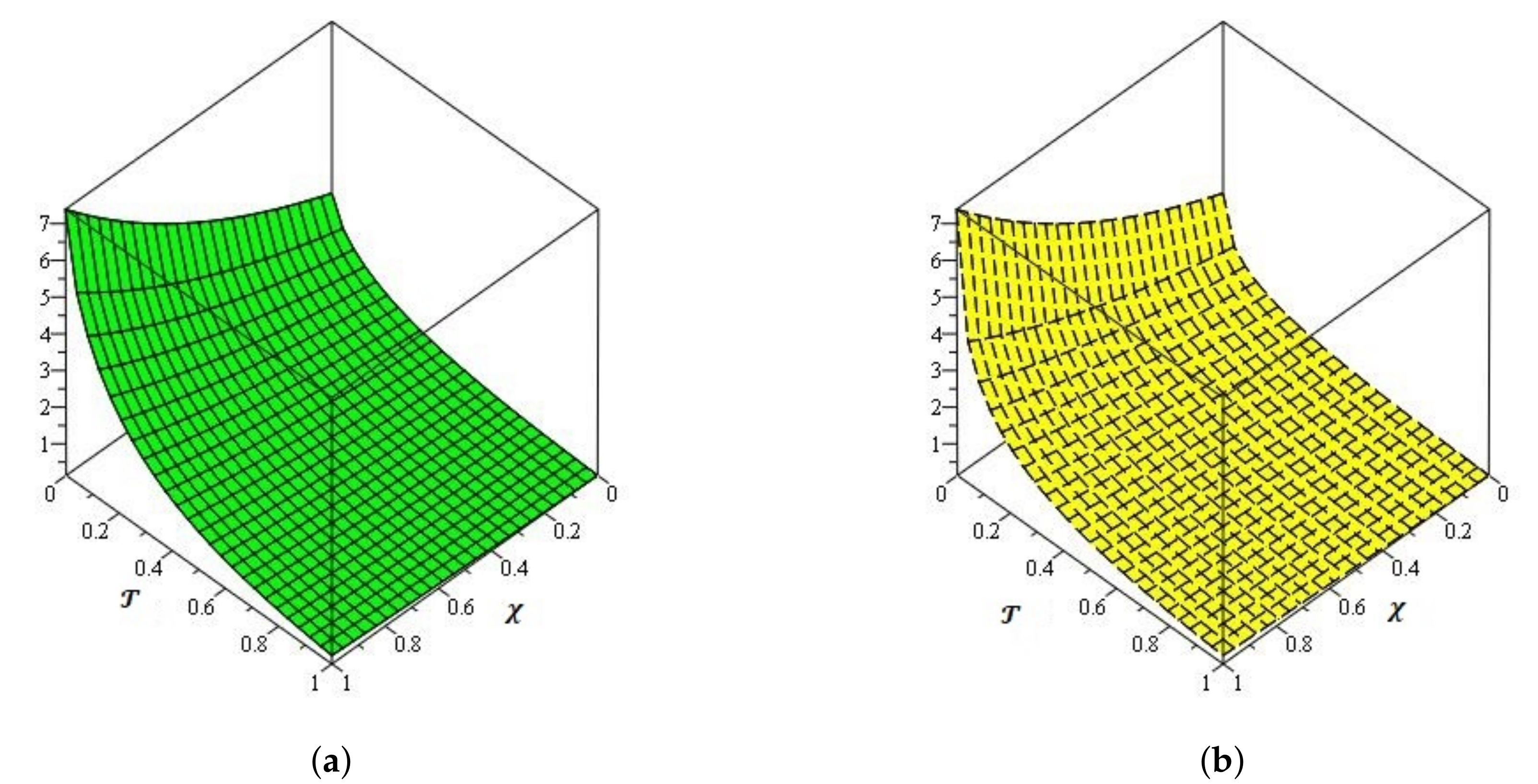
The EDM and the exact results of Problem 1 at $\delta =2$ are shown in Figure 1 by plots (a) and (b) respectively. It can be seen from the given figures that both the precise and the EDM outcomes are in near touch with each other. The EDM effects of Example 1 are also measured in Figure 2a,b at separate fractional-order $\delta =1.7$ and $1.5$. It is examined that the outcomes of the example of fractional order are convergent as fractional-order analysis of integer-order to an integer-order outcome. The same process of convergence of solutions of fractional order into solutions of integral order is found.

Example 2. 

Consider the fractional-order two dimensional telegraph equation [9]:

$$\frac{{\partial }^{2\delta }\mu }{\partial {{\mathcal{T}}_1}^{2\delta }}+3\frac{{\partial }^{\delta }\mu }{\partial {{\mathcal{T}}_1}^{\delta }}+2\mu =\frac{{\partial }^2\mu }{\partial {{\mathcal{X}}_1}^2}+\frac{{\partial }^2\mu }{\partial {{\mathcal{Y}}_1}^2},\hspace{1em}\hspace{1em}0<\delta \le 1,\hspace{1em}\hspace{1em}t\ge 0,$$

(17)

with the initial conditions

$$\mu ({\mathcal{X}}_1,{\mathcal{Y}}_1,0)=e^{{\mathcal{X}}_1+{\mathcal{Y}}_1},\hspace{1em}\hspace{1em}{\mu }_{{\mathcal{X}}_1}({\mathcal{X}}_1,{\mathcal{Y}}_1,0)=-3e^{{\mathcal{X}}_1+{\mathcal{Y}}_1}.$$

(18)

Applying the Elzaki transformation of Equation (18),

$$E\left[\frac{{\partial }^{2\delta }\mu }{\partial {{\mathcal{T}}_1}^{2\delta }}\right]=-E\left[3\frac{{\partial }^{\delta }\mu }{\partial {{\mathcal{T}}_1}^{\delta }}+2\mu -\frac{{\partial }^2\mu }{\partial {{\mathcal{X}}_1}^2}-\frac{{\partial }^2\mu }{\partial {{\mathcal{Y}}_1}^2}\right],$$

$$s^{\delta }E\left[\mu ({\mathcal{X}}_1,{\mathcal{Y}}_1,{\mathcal{T}}_1)\right]-s^{2-\delta }\mu ({\mathcal{X}}_1,{\mathcal{Y}}_1,0)-s^{3-\delta }{\mu }_{{\mathcal{X}}_1}({\mathcal{X}}_1,{\mathcal{Y}}_1,0)=-E\left[3\frac{{\partial }^{\delta }\mu }{\partial {{\mathcal{T}}_1}^{\delta }}+2\mu -\frac{{\partial }^2\mu }{\partial {{\mathcal{X}}_1}^2}-\frac{{\partial }^2\mu }{\partial {{\mathcal{Y}}_1}^2}\right].$$

Using the inverse Elzaki transformation

$$\mu ({\mathcal{X}}_1,{\mathcal{Y}}_1,{\mathcal{T}}_1)=E^{-1}\left[s^2\mu ({\mathcal{X}}_1,{\mathcal{Y}}_1,0)+s^3{\mu }_{{\mathcal{X}}_1}({\mathcal{X}}_1,{\mathcal{Y}}_1,0)-s^{\delta }E\left\{3\frac{{\partial }^{\delta }\mu }{\partial {{\mathcal{T}}_1}^{\delta }}+2\mu -\frac{{\partial }^2\mu }{\partial {{\mathcal{X}}_1}^2}-\frac{{\partial }^2\mu }{\partial {{\mathcal{Y}}_1}^2}\right\}\right].$$

Implementing the ADM process, we have

$$\begin{array}{c}{\mu }_0({\mathcal{X}}_1,{\mathcal{Y}}_1,{\mathcal{T}}_1)=E^{-1}\left[s^2\mu ({\mathcal{X}}_1,{\mathcal{Y}}_1,0)+s^3{\mu }_{{\mathcal{X}}_1}({\mathcal{X}}_1,{\mathcal{Y}}_1,0)\right]=E^{-1}\left[s^2{e}^{{\mathcal{X}}_1+{\mathcal{Y}}_1}-s^{3}3e^{{\mathcal{X}}_1+{\mathcal{Y}}_1}\right],\\ {\mu }_0({\mathcal{X}}_1,{\mathcal{Y}}_1,{\mathcal{T}}_1)=e^{{\mathcal{X}}_1+{\mathcal{Y}}_1}(1-3{\mathcal{T}}_1),\\ {\mu }_{j+1}({\mathcal{X}}_1,{\mathcal{Y}}_1,{\mathcal{T}}_1)=-E^{-1}\left[s^{\delta }E\left\{3\frac{{\partial }^{\delta }{\mu }_j}{\partial {{\mathcal{T}}_1}^{\delta }}+2{\mu }_j-\frac{{\partial }^2{\mu }_j}{\partial {{\mathcal{X}}_1}^2}-\frac{{\partial }^2{\mu }_j}{\partial {{\mathcal{Y}}_1}^2}\right\}\right],\hspace{1em}\hspace{1em}j=0,1,2,\cdots \end{array}$$

(19)

for $j=0$

$$\begin{array}{c}{\mu }_1({\mathcal{X}}_1,{\mathcal{Y}}_1,{\mathcal{T}}_1)=-E^{-1}\left[s^{\delta }E\left\{3\frac{{\partial }^{\delta }{\mu }_0}{\partial {{\mathcal{T}}_1}^{\delta }}+2{\mu }_0-\frac{{\partial }^2{\mu }_0}{\partial {{\mathcal{X}}_1}^2}-\frac{{\partial }^2{\mu }_0}{\partial {{\mathcal{Y}}_1}^2}\right\}\right],\hfill \\ {\mu }_1({\mathcal{X}}_1,{\mathcal{Y}}_1,{\mathcal{T}}_1)=9e^{{\mathcal{X}}_1+{\mathcal{Y}}_1}\frac{{{\mathcal{T}}_1}^{\delta +1}}{\mathrm{\Gamma }(\delta +2)}.\hfill \end{array}$$

(20)

$$\begin{array}{c}{\mu }_2({\mathcal{X}}_1,{\mathcal{T}}_1)=-E^{-1}\left[s^{\delta }E\left\{3\frac{{\partial }^{\delta }{\mu }_1}{\partial {{\mathcal{T}}_1}^{\delta }}+2{\mu }_1-\frac{{\partial }^2{\mu }_1}{\partial {{\mathcal{X}}_1}^2}-\frac{{\partial }^2{\mu }_1}{\partial {{\mathcal{Y}}_1}^2}\right\}\right]=-27e^{{\mathcal{X}}_1+{\mathcal{Y}}_1}\frac{{{\mathcal{T}}_1}^{2\delta +1}}{\mathrm{\Gamma }(2\delta +2)},\hfill \\ {\mu }_3({\mathcal{X}}_1,{\mathcal{T}}_1)=-E^{-1}\left[s^{\delta }E\left\{3\frac{{\partial }^{\delta }{\mu }_2}{\partial {{\mathcal{T}}_1}^{\delta }}+2{\mu }_2-\frac{{\partial }^2{\mu }_2}{\partial {{\mathcal{X}}_1}^2}-\frac{{\partial }^2{\mu }_2}{\partial {{\mathcal{Y}}_1}^2}\right\}\right]=81e^{{\mathcal{X}}_1+{\mathcal{Y}}_1}\frac{{{\mathcal{T}}_1}^{3\delta +1}}{\mathrm{\Gamma }(3\delta +2)}.\hfill \\ ⋮\hfill \end{array}$$

(21)

The EDM result for Problem 2 is

$$\mu ({\mathcal{X}}_1,{\mathcal{Y}}_1,{\mathcal{T}}_1)={\mu }_0({\mathcal{X}}_1,{\mathcal{T}}_1)+{\mu }_1({\mathcal{X}}_1,{\mathcal{T}}_1)+{\mu }_2({\mathcal{X}}_1,{\mathcal{T}}_1)+{\mu }_3({\mathcal{X}}_1,{\mathcal{T}}_1)+{\mu }_4({\mathcal{X}}_1,{\mathcal{T}}_1)\cdots$$

$$\mu ({\mathcal{X}}_1,{\mathcal{T}}_1)=e^{{\mathcal{X}}_1+{\mathcal{Y}}_1}\left[1-3{\mathcal{T}}_1+9\frac{{{\mathcal{T}}_1}^{\delta +1}}{\mathrm{\Gamma }(\delta +2)}-27\frac{{{\mathcal{T}}_1}^{2\delta +1}}{\mathrm{\Gamma }(2\delta +2)}+81\frac{{{\mathcal{T}}_1}^{3\delta +1}}{\mathrm{\Gamma }(3\delta +2)}\cdots \right],$$

when $\delta =2$, then EDM result is

$$\mu ({\mathcal{X}}_1,{\mathcal{Y}}_1,{\mathcal{T}}_1)=e^{{\mathcal{X}}_1+{\mathcal{Y}}_1}\left[1-3{\mathcal{T}}_1+\frac{{\left(3{\mathcal{T}}_1\right)}^2}{2!}-\frac{{\left(3{\mathcal{T}}_1\right)}^3}{3!}+\frac{{\left(3{\mathcal{T}}_1\right)}^4}{4!}\cdots \right].$$

(22)

The exact result of Equation (18):

$$\mu ({\mathcal{X}}_1,{\mathcal{Y}}_1,{\mathcal{T}}_1)=e^{{\mathcal{X}}_1+{\mathcal{Y}}_1-3{\mathcal{T}}_1}.$$

The EDM and the exact results of Problem 1 at $\delta =2$ are shown in Figure 3 by plots (a) and (b) respectively. It can be seen from the given figures that both the precise and the EDM outcomes are in near touch with each other. The EDM effects of Example 1 are also measured in Figure 4a,b at separate fractional-order $\delta =1.7$ and $1.5$. It is examined that the outcomes of the example of fractional order are convergent as fractional-order analysis of integer-order to an integer-order outcome. The same process of convergence of solutions of fractional order into solutions of integral order is found.

Example 3. 

Consider the fractional-order three dimensional telegraph equation [9]:

$$\frac{{\partial }^{2\delta }\mu }{\partial {{\mathcal{T}}_1}^{2\delta }}+2\frac{{\partial }^{\delta }\mu }{\partial {{\mathcal{T}}_1}^{\delta }}+3\mu =\frac{{\partial }^2\mu }{\partial {{\mathcal{X}}_1}^2}+\frac{{\partial }^2\mu }{\partial {{\mathcal{Y}}_1}^2}+\frac{{\partial }^2\mu }{\partial {{\mathcal{Z}}_1}^2},\hspace{1em}\hspace{1em}0<\delta \le 1,\hspace{1em}\hspace{1em}t\ge 0,$$

(23)

with the initial conditions

$$\begin{array}{c}\mu ({\mathcal{X}}_1,{\mathcal{Y}}_1,{\mathcal{Z}}_1,0)=\sinh \left({\mathcal{X}}_1\right)\sinh \left({\mathcal{Y}}_1\right)\sinh \left({\mathcal{Z}}_1\right),\hfill \\ {\mu }_{{\mathcal{T}}_1}({\mathcal{X}}_1,{\mathcal{Y}}_1,{\mathcal{Z}}_1,0)=-\sinh \left({\mathcal{X}}_1\right)\sinh \left({\mathcal{Y}}_1\right)\sinh \left({\mathcal{Z}}_1\right).\hfill \end{array}$$

(24)

Applying the Elzaki transform of Equation (24),

$$E\left[\frac{{\partial }^{2\delta }\mu }{\partial {{\mathcal{T}}_1}^{2\delta }}\right]=-E\left[2\frac{{\partial }^{\delta }\mu }{\partial {{\mathcal{T}}_1}^{\delta }}+3\mu -\frac{{\partial }^2\mu }{\partial {{\mathcal{X}}_1}^2}-\frac{{\partial }^2\mu }{\partial {{\mathcal{Y}}_1}^2}-\frac{{\partial }^2\mu }{\partial {{\mathcal{Z}}_1}^2}\right],$$

$$\begin{array}{cc}& s^{\delta }E\left[\mu ({\mathcal{X}}_1,{\mathcal{Y}}_1,{\mathcal{Z}}_1,{\mathcal{T}}_1)\right]-s^{2-\delta }\mu ({\mathcal{X}}_1,{\mathcal{Y}}_1,{\mathcal{Z}}_1,0)-s^{3-\delta }{\mu }_{{\mathcal{X}}_1}({\mathcal{X}}_1,{\mathcal{Y}}_1,{\mathcal{Z}}_1,0)=-E\left[2\frac{{\partial }^{\delta }\mu }{\partial {{\mathcal{T}}_1}^{\delta }}+3\mu -\frac{{\partial }^2\mu }{\partial {{\mathcal{X}}_1}^2}-\frac{{\partial }^2\mu }{\partial {{\mathcal{Y}}_1}^2}-\frac{{\partial }^2\mu }{\partial {{\mathcal{Z}}_1}^2}\right].\hfill \end{array}$$

Using the inverse Elzaki transform

$$\begin{array}{cc}\hfill \mu ({\mathcal{X}}_1,{\mathcal{Y}}_1,{\mathcal{Z}}_1,{\mathcal{T}}_1)=& E^{-1}\left[s^2\mu ({\mathcal{X}}_1,{\mathcal{Y}}_1,{\mathcal{Z}}_1,0)+s^3{\mu }_{{\mathcal{X}}_1}({\mathcal{X}}_1,{\mathcal{Y}}_1,{\mathcal{Z}}_1,0)\right]\hfill \\ & -E^{-1}\left[s^{\delta }E\left\{2\frac{{\partial }^{\delta }\mu }{\partial {{\mathcal{T}}_1}^{\delta }}+3\mu -\frac{{\partial }^2\mu }{\partial {{\mathcal{X}}_1}^2}-\frac{{\partial }^2\mu }{\partial {{\mathcal{Y}}_1}^2}-\frac{{\partial }^2\mu }{\partial {{\mathcal{Z}}_1}^2}\right\}\right].\hfill \end{array}$$

Implementing the ADM procedure, we get

$$\begin{array}{c}{\mu }_0({\mathcal{X}}_1,{\mathcal{Y}}_1,{\mathcal{Z}}_1,{\mathcal{T}}_1)=E^{-1}\left[s^2\mu ({\mathcal{X}}_1,{\mathcal{Y}}_1,{\mathcal{Z}}_1,0)+s^3{\mu }_{{\mathcal{X}}_1}({\mathcal{X}}_1,{\mathcal{Y}}_1,{\mathcal{Z}}_1,0)\right]\\ =E^{-1}\left[s^2\sinh \left({\mathcal{X}}_1\right)\sinh \left({\mathcal{Y}}_1\right)\sinh \left({\mathcal{Z}}_1\right)-s^3\sinh \left({\mathcal{X}}_1\right)\sinh \left({\mathcal{Y}}_1\right)\sinh \left({\mathcal{Z}}_1\right)\right],\\ {\mu }_0({\mathcal{X}}_1,{\mathcal{Y}}_1,{\mathcal{Z}}_1,{\mathcal{T}}_1)=\sinh \left({\mathcal{X}}_1\right)\sinh \left({\mathcal{Y}}_1\right)\sinh \left({\mathcal{Z}}_1\right)(1-{\mathcal{T}}_1),\\ {\mu }_{j+1}({\mathcal{X}}_1,{\mathcal{Y}}_1,{\mathcal{Z}}_1,{\mathcal{T}}_1)=-E^{-1}\left[s^{\delta }E\left\{2\frac{{\partial }^{\delta }{\mu }_j}{\partial {{\mathcal{T}}_1}^{\delta }}+3{\mu }_j-\frac{{\partial }^2{\mu }_j}{\partial {{\mathcal{X}}_1}^2}-\frac{{\partial }^2{\mu }_j}{\partial {{\mathcal{Y}}_1}^2}-\frac{{\partial }^2{\mu }_j}{\partial {{\mathcal{Z}}_1}^2}\right\}\right],\hspace{1em}j=0,1,2,\cdots \end{array}$$

(25)

for$j=0$

$$\begin{array}{c}{\mu }_1({\mathcal{X}}_1,{\mathcal{Y}}_1,{\mathcal{Z}}_1,{\mathcal{T}}_1)=-E^{-1}\left[s^{\delta }E\left\{2\frac{{\partial }^{\delta }{\mu }_0}{\partial {{\mathcal{T}}_1}^{\delta }}+3{\mu }_0-\frac{{\partial }^2{\mu }_0}{\partial {{\mathcal{X}}_1}^2}-\frac{{\partial }^2{\mu }_0}{\partial {{\mathcal{Y}}_1}^2}-\frac{{\partial }^2{\mu }_0}{\partial {{\mathcal{Z}}_1}^2}\right\}\right],\hfill \\ {\mu }_1({\mathcal{X}}_1,{\mathcal{Y}}_1,{\mathcal{Z}}_1,{\mathcal{T}}_1)=-2\sinh \left({\mathcal{X}}_1\right)\sinh \left({\mathcal{Y}}_1\right)\sinh \left({\mathcal{Z}}_1\right)\frac{{{\mathcal{T}}_1}^{\delta +1}}{\gamma (\delta +2)},\hfill \end{array}$$

(26)

$$\begin{array}{c}{\mu }_2({\mathcal{X}}_1,{\mathcal{Y}}_1,{\mathcal{Z}}_1,{\mathcal{T}}_1)=-E^{-1}\left[s^{\delta }E\left\{2\frac{{\partial }^{\delta }{\mu }_1}{\partial {{\mathcal{T}}_1}^{\delta }}+3{\mu }_1-\frac{{\partial }^2{\mu }_1}{\partial {{\mathcal{X}}_1}^2}-\frac{{\partial }^2{\mu }_1}{\partial {{\mathcal{Y}}_1}^2}-\frac{{\partial }^2{\mu }_1}{\partial {{\mathcal{Z}}_1}^2}\right\}\right],\hfill \\ {\mu }_2({\mathcal{X}}_1,{\mathcal{Y}}_1,{\mathcal{Z}}_1,{\mathcal{T}}_1)=4\sinh \left({\mathcal{X}}_1\right)\sinh \left({\mathcal{Y}}_1\right)\sinh \left({\mathcal{Z}}_1\right)\frac{{{\mathcal{T}}_1}^{2\delta +1}}{\mathrm{\Gamma }(2\delta +2)},\hfill \\ {\mu }_3({\mathcal{X}}_1,{\mathcal{Y}}_1,{\mathcal{Z}}_1,{\mathcal{T}}_1)=-E^{-1}\left[s^{\delta }E\left\{2\frac{{\partial }^{\delta }{\mu }_2}{\partial {{\mathcal{T}}_1}^{\delta }}+3{\mu }_2-\frac{{\partial }^2{\mu }_2}{\partial {{\mathcal{X}}_1}^2}-\frac{{\partial }^2{\mu }_2}{\partial {{\mathcal{Y}}_1}^2}-\frac{{\partial }^2{\mu }_2}{\partial {{\mathcal{Z}}_1}^2}\right\}\right],\hfill \\ {\mu }_3({\mathcal{X}}_1,{\mathcal{Y}}_1,{\mathcal{Z}}_1,{\mathcal{T}}_1)=-8\sinh \left({\mathcal{X}}_1\right)\sinh \left({\mathcal{Y}}_1\right)\sinh \left({\mathcal{Z}}_1\right)\frac{{{\mathcal{T}}_1}^{3\delta +1}}{\mathrm{\Gamma }(3\delta +2)}.\hfill \\ ⋮\hfill \end{array}$$

(27)

The EDM result for Example 3 is

$$\mu ({\mathcal{X}}_1,{\mathcal{Y}}_1,{\mathcal{Z}}_1,{\mathcal{T}}_1)={\mu }_0({\mathcal{X}}_1,{\mathcal{Y}}_1,{\mathcal{Z}}_1,{\mathcal{T}}_1)+{\mu }_1({\mathcal{X}}_1,{\mathcal{Y}}_1,{\mathcal{Z}}_1,{\mathcal{T}}_1)+{\mu }_2({\mathcal{X}}_1,{\mathcal{Y}}_1,{\mathcal{Z}}_1,{\mathcal{T}}_1)+{\mu }_3({\mathcal{X}}_1,{\mathcal{Y}}_1,{\mathcal{Z}}_1,{\mathcal{T}}_1)\cdots .$$

$$\mu ({\mathcal{X}}_1,{\mathcal{Y}}_1,{\mathcal{Z}}_1,{\mathcal{T}}_1)=\sinh \left({\mathcal{X}}_1\right)\sinh \left({\mathcal{Y}}_1\right)\sinh \left({\mathcal{Z}}_1\right)\left[1+{\mathcal{T}}_1-2\frac{{{\mathcal{T}}_1}^{\delta +1}}{\mathrm{\Gamma }(\delta +2)}+4\frac{{{\mathcal{T}}_1}^{2\delta +1}}{\mathrm{\Gamma }(2\delta +2)}-8\frac{{{\mathcal{T}}_1}^{3\delta +1}}{\mathrm{\Gamma }(3\delta +2)}\cdots \right].$$

The exact result of Equation (24):

$$\mu ({\mathcal{X}}_1,{\mathcal{Y}}_1,{\mathcal{Z}}_1,{\mathcal{T}}_1)=e^{-2{\mathcal{T}}_1}\sinh \left({\mathcal{X}}_1\right)\sinh \left({\mathcal{Y}}_1\right)\sinh \left({\mathcal{Z}}_1\right).$$

The EDM and the exact results of Problem 1 at $\delta =2$ are shown in Figure 5 by plots (a) and (b) respectively. It can be seen from the given figures that both the precise and the EDM outcomes are in near touch with each other. The EDM effects of Example 1 are also measured in Figure 6a,b at separate fractional-order $\delta =1.7$ and $1.5$. It is examined that the outcomes of the example of fractional order are convergent as fractional-order analysis of integer-order to an integer-order outcome. The same process of convergence of solutions of fractional order into solutions of integral order is found.

5. Conclusions

In this paper, we analyzed the time-fractional telegraph equations, using an Elzaki decomposition technique. Using the proposed method, the solutions for certain illustrative examples are clarified. The graphical analysis of the fractional-order solutions acquired verified the convergence towards the integer order solutions. In addition, the present method is simple, straightforward and less computational cost and the suggested method to solve other fractional-order partial differential equations.

References

- Podlubny, I. Fractional Differential Equations. In Mathematics in Science and Engineering; Academic Press: San Diego, CA, USA, 1999; Volume 198. [Google Scholar]
- Hilfer, R. Applications of Fractional Calculus in Physics; World Scientific Publishing: River Edge, NJ, USA, 2000. [Google Scholar]
- Ibrahim, R.W. On holomorphic solution for space-and time-fractional telegraph equations in complex domain. J. Funct. Spaces Appl. 2012, 2012, 703681. [Google Scholar] [CrossRef]
- Zhang, Y.; Liu, X.; Belic, M.R.; Zhong, W.; Zhang, Y.; Xiao, M. Propagation dynamics of a light beam in a fractional Schrodinger equation. Phys. Rev. Lett. 2015, 115, 180403. [Google Scholar] [CrossRef] [PubMed]
- Zhang, Y.; Zhong, H.; Belic, M.R.; Zhu, Y.; Zhong, W.; Zhang, Y.; Christodoulides, D.N.; Xiao, M. PT symmetry in a fractional Schrodinger equation. Laser Photonics Rev. 2016, 10, 526–531. [Google Scholar] [CrossRef] [Green Version]
- Javidi, M.; Nyamoradi, N. Numerical solution of telegraph equation by using LT inversion technique. Int. J. Adv. Math. Sci. 2013, 1, 64–77. [Google Scholar] [CrossRef] [Green Version]
- Veeresha, P.; Prakasha, D.G. Numerical solution for fractional model of telegraph equation by using q-HATM. arXiv 2018, arXiv:1805.03968. [Google Scholar]
- Al-badrani, H.; Saleh, S.; Bakodah, H.O.; Al-Mazmumy, M. Numerical Solution for Nonlinear Telegraph Equation by Modified Adomian Decomposition Method. Nonlinear Anal. Differ. Equ. 2016, 4, 243–257. [Google Scholar] [CrossRef]
- Srivastava, V.K.; Awasthi, M.K.; Tamsir, M. RDTM solution of Caputo time fractional-order hyperbolic telegraph equation. Aip Adv. 2013, 3, 032142. [Google Scholar] [CrossRef] [Green Version]
- Inc, M.; Akgul, A.; Kilicman, A. Explicit solution of telegraph equation based on reproducing kernel method. J. Funct. Spaces Appl. 2012, 2012, 984682. [Google Scholar] [CrossRef] [Green Version]
- Biazar, J.; Ebrahimi, H.; Ayati, Z. An approximation to the solution of telegraph equation by variational iteration method. Numer. Methods Partial. Differ. Equ. 2009, 25, 797–801. [Google Scholar] [CrossRef]
- Erfanian, M.; Gachpazan, M. A new method for solving of telegraph equation with Haar wavelet. Int. J. Math. Comput. Sci. 2016, 3, 6–10. [Google Scholar]
- Latifizadeh, H. The sinc-collocation method for solving the telegraph equation. J. Comput. Inform. 2013, 1, 13–17. [Google Scholar]
- Elzaki, T.M. The new integral transform Elzaki transform. Glob. J. Pure Appl. Math. 2011, 7, 57–64. [Google Scholar]
- Elzaki, T.M. On the connections between Laplace and Elzaki transforms. Adv. Theor. Appl. Math. 2011, 6, 1–11. [Google Scholar]
- Elzaki, T.M. On The New Integral Transform “Elzaki Transform” Fundamental Properties Investigations and Applications. Glob. J. Math. Sci. Theory Pract. 2012, 4, 1–13. [Google Scholar]
- Jena, R.M.; Chakraverty, S. Solving time-fractional Navier-Stokes equations using homotopy perturbation Elzaki transform. SN Appl. Sci. 2019, 1, 16. [Google Scholar] [CrossRef] [Green Version]
- Sedeeg, A.K.H. A coupling Elzaki transform and homotopy perturbation method for solving nonlinear fractional heat-like equations. Am. J. Math. Comput. Model. 2016, 1, 15–20. [Google Scholar]
- Neamaty, A.; Agheli, B.; Darzi, R. Applications of homotopy perturbation method and Elzaki transform for solving nonlinear partial differential equations of fractional order. J. Nonlinear Evol. Equ. Appl. 2016, 2015, 91–104. [Google Scholar]
- Miller, K.S.; Ross, B. An Introduction to the Fractional Calculus and Fractional Differential Equations; Wiley: New York, NY, USA, 1993. [Google Scholar]
- Podlubny, I. Fractional Differential Equations: An Introduction to Fractional Derivatives, Fractional Differential Equations, to Methods of Their Solution and Some of Their Applications; Elsevier, Academic Press: San Diego, CA, USA, 1998; Volume 198. [Google Scholar]
- Hilfer, R. (Ed.) Applications of Fractional Calculus in Physics; World Scientific: Singapore, 2000; Volume 35, pp. 87–130. [Google Scholar]
Figure 1.
(a) The graph of exact result of Problem 1. (b) The graph of analytical result of problem 1 for δ = 2.
Figure 2.
(a) The graph of analytical result of Problem 1 for δ = 1.7. (b) The graph of analytical result of Problem 1 for δ = 1.5.
Figure 3.
(a) The graph of exact result of Problem 2. (b) The graph of analytical result of Problem 2 for δ = 2.
Figure 4.
(a) The graph of analytical result of Problem 2 for δ = 1.7. (b) The graph of analytical result of Problem 2 for δ = 1.5.
Figure 5.
(a) The graph of exact result of Problem 3. (b) The graph of analytical result of Problem 3 for δ = 2.
Figure 6.
(a) The graph of analytical result of Problem 3 for δ = 1.7. (b) The graph of analytical result of Problem 3 for δ = 1.5
Publisher’s Note: MDPI stays neutral with regard to jurisdictional claims in published maps and institutional affiliations. |
© 2020 by the authors. Licensee MDPI, Basel, Switzerland. This article is an open access article distributed under the terms and conditions of the Creative Commons Attribution (CC BY) license (http://creativecommons.org/licenses/by/4.0/).
Share and Cite
MDPI and ACS Style
Shah, N.A.; Dassios, I.; Chung, J.D. A Decomposition Method for a Fractional-Order Multi-Dimensional Telegraph Equation via the Elzaki Transform. Symmetry 2021, 13, 8. https://doi.org/10.3390/sym13010008
AMA Style
Shah NA, Dassios I, Chung JD. A Decomposition Method for a Fractional-Order Multi-Dimensional Telegraph Equation via the Elzaki Transform. Symmetry. 2021; 13(1):8. https://doi.org/10.3390/sym13010008
Chicago/Turabian StyleShah, Nehad Ali, Ioannis Dassios, and Jae Dong Chung. 2021. "A Decomposition Method for a Fractional-Order Multi-Dimensional Telegraph Equation via the Elzaki Transform" Symmetry 13, no. 1: 8. https://doi.org/10.3390/sym13010008
Note that from the first issue of 2016, this journal uses article numbers instead of page numbers. See further details here.