
Determination of Critical Loads for Eutrophying and Acidifying Air Pollutant Inputs for the Protection of Near-Natural Ecosystems in Germany

1
IBE/ÖKO-DATA-Dr. Eckhof Consulting/Ecosystem Analysis and Environmental Data Management, Lessingstraße 16, 16356 Ahrensfelde, Germany
2
German Federal Environment Agency, P.O. Box 14 06, 06813 Dessau-Roßlau, Germany
*
Author to whom correspondence should be addressed.
Atmosphere 2023, 14(2), 383; https://doi.org/10.3390/atmos14020383
Submission received: 20 December 2022
/
Revised: 7 February 2023
/
Accepted: 13 February 2023
/
Published: 15 February 2023
(This article belongs to the Special Issue Atmospheric Deposition and Its Effects on Terrestrial Ecosystems)
Abstract
:Under the Convention on Long-Range Transboundary Air Pollution (CLRTAP) of the UN Economic Commission for Europe, UNECE, to which Germany acceded in 1982, the harmful effects of air pollutants on the environment are to be steadily reduced and ultimately limited to a level that is compatible with nature. The ICP Modelling & Mapping (ICP M&M) under the Working Group on Effects (WGE) of CLRTAP maps critical loads for the entire Convention area and calculates the exceedance risks and associated risks to vegetation and biodiversity. A current data request was made in November 2015 with the aim of submitting new or updated ecosystem-specific critical loads for protection against acidification and eutrophication. For this task, critical loads were determined by the authors for one third of the territory of Germany using the simple mass balance (SMB) method according to the ICP Mapping Manual. The permissible eutrophying nitrogen input into the ecosystem CLnut(N), as well as the acidifying sulphur input CLmaxS, can be described as the setting of the equilibrium between substance inputs and outputs, provided that specific critical limits are met. The BERN database—created by the authors—serves as the basis for modelling vegetation-specific critical limits as a complement to the SMB model. The BERN database contains near-natural plant communities with clearly definable site constancy. The 25,600 German and a further 24,600 European vegetation records dating back to before 1960 were evaluated to determine the good ecological status of the plant communities. The results of the critical load calculation show that about half of the receptor areas have critical loads for eutrophying nitrogen below 10 kg ha−1 a−1 and critical loads for acidifying sulphur were below 1500 eq ha−1 a−1. It could be demonstrated that the BERN–SMB-modelled critical loads for eutrophying nitrogen inputs show lower values on average throughout Germany than those calculated using only the previous critical limits according to the ICP Mapping Manual. These values are closer to the empirical critical loads than the critical loads without BERN data. For the goal of the German National Biodiversity Strategy by 2007 and 2020 to define ecosystem-related impact thresholds for pollutants that describe the effects on biodiversity, the BERN/SMB critical loads for the protection of ecosystems provide a precautionary scientific basis.
1. Introduction
Under the Convention on Long-range Transboundary Air Pollution (CLRTAP) of the UN Economic Commission for Europe, UNECE [1], to which Germany acceded in 1982, the harmful effects of air pollutants on humans and the environment are to be steadily reduced and ultimately avoided.
For terrestrial ecosystems, air pollutants, along with climate change, are a major risk factor and threaten the preservation of biodiversity in Germany. Since the 1980s, therefore, the input of pollutants from the air has been analyzed and the resulting hazards assessed. In particular, acidification through sulphur and nitrogen compounds, as well as excessive nutrient inputs (eutrophication), which occur through oxidized nitrogen (nitrogen oxides) and reduced nitrogen (ammonia), are to be limited to a level that is compatible with nature.
The German government has ratified the Gothenburg Protocol (the 1999 Gothenburg Protocol to Abate Acidification, Eutrophication and Ground-level Ozone), named after its place of signature, as well as the other seven protocols to the Convention on Long-range Transboundary Air Pollution (CLRTAP) [1]. The Gothenburg Protocol, also known as the Multicomponent Protocol, entered into force in 2005. The Gothenburg Protocol was revised in 2012 [2]. It is undisputed that this Protocol has played a major role in significantly reducing the environmental impact of air pollutants in Europe over the last 35 years.
The Commission of the European communities (EC) also presented a new package of measures for clean air for Europe at the end of 2013 to update the existing legislation [3]. Part of the package is a “Clean Air for Europe” program [4], which initially aims to ensure compliance with existing targets. In addition, new air quality targets for 2030 are also formulated. A revised directive on national emission ceilings or national emission reduction commitments was also adopted. This new Directive (EU) 2016/2284 of the European Parliament and of the Council of 14 December 2016 [5], now referred to as the NERC Directive (NERC = National Emission Reduction Commitments) contains targets for the six most important air pollutants and measures to be realized between 2020 and 2030. Here, too, ambitious targets have been set for Germany.
The two aforementioned sets of regulations are intended to minimize the damaging effects of eutrophication and acidification in Europe in particular, in addition to other environmental burdens. The emission ceilings or percentage reduction obligations of both sets of regulations are based on reduction targets that are derived from critical pollutant input rates into ecosystems (critical loads) and their compliance or exceedance. According to current knowledge, compliance with or undercutting of such critical loads guarantees that a selected protected good, the ecological receptor, will not be damaged either acutely or in the long term.
The ICP Modelling & Mapping (ICP M&M) under the Working Group on Effects (WGE) of CLRTAP [6] maps critical loads for the entire Convention area and calculates the exceedance risks and associated risks to vegetation and biodiversity [7]. The Coordination Centre for Effects (CCE) acts as data hub for the ICP M&M [8]. It is also responsible for keeping the critical load approach up to date and ensuring the methods and equations are updated to present knowledge if needed. The National Focal Centres (NFC) provide national data to the CCE for the assessment of acidification and eutrophication risks and for biodiversity conservation. Accordingly, the NFCs have to respond to the “Call for Data” (CFD) issued by the ICP M&M. A current data request was made in November 2015 with the aim of submitting new or updated ecosystem-specific critical loads for protection against acidification and eutrophication [9].
The basic principles for modelling critical loads (CL) are published by the International Co-operative Programme on Modelling and Mapping of Critical Loads and Levels and Air Pollution Effects, Risks and Trends (ICP Modelling & Mapping) in a Mapping Manual [10,11]. The National Focal Centers (NFC) are responsible for data submissions of their individual countries and also for following the Mapping Manual when modelling CL. When properly documented, the NFC have the opportunity to expand, modify or specify the methods of the Mapping Manual with national approaches.
Currently, three different methods are used internationally to determine critical N and S input rates as state of the art:
- (1)
- Empirical critical loads for nitrogen were last compiled at an expert workshop in Bern 2022 [12]. The empirical approaches use dose-response relationships based on experience and field studies to assign pollutant input limits to a specific ecological receptor or a defined ecosystem. This allocation table using the EUNIS codes for the different ecosystem types occurring in Europe contains information on empirical critical loads for eutrophying nitrogen based on nitrogen addition experiments, long-term observations or expert opinions. As a rule, these critical loads are given as ranges of values for EUNIS classes. However, not all relevant EUNIS classes are included in the list of empirical critical loads. The simple approach of empirically deriving cause–effect relationships between the nitrogen input and the response of relatively roughly classified vegetation types is particularly suitable for large-scale extrapolations, as comparatively few data are required. The often wide ranges also usually offer a broad scope for interpretation.
- (2)
- According to the simple mass balance (SMB) method [11], the permissible eutrophying nitrogen input into the ecosystem CLnut(N), as well as the acidifying sulphur input CLmaxS can be described as the setting of the equilibrium between substance inputs and outputs, provided that specific critical limits are met. Temporary deviations from the state of equilibrium can only be tolerated as long as the system remains capable of self-regeneration (quasi-steady state). This deterministic and process-based approach simulates the biotic and ecological changes with the help of a mathematical model representation of the most important processes in the ecosystem. However, the mathematical equations used cannot be better than the knowledge of the ecological processes on which they are based.
- (3)
- Dynamic modelling approaches reproduce the changes in vegetation as a function of changing abiotic site factors or forecast them into the future. The most commonly used models are two-stage in that the geochemical processes are simulated first, and their results are then used as drivers in the biotic models [13]. In order to determine critical loads with the help of dynamic models, it is necessary to set parameter values that are to be achieved in the desired target state. Dynamic modelling is primarily suitable for individual sites, as a large amount of input data is required, which can often only be determined with great effort.
The German Federal Environment Agency performs the tasks of a National Focal Center for Germany, and the Company for Ecosystem Analysis and Environmental Data Management (ÖKO-DATA) was commissioned as the national data center to provide technical support and data preparation. For this task, ÖKO-DATA determined critical loads for one third of the territory of Germany (Table 1) using the simple mass balance (SMB) method [14].
The critical limits used in the SMB approach were first determined according to the recommendations in the Mapping Manual [10,11]. In addition, an approach for determining the vegetation-specific critical limits was tested, which differentiates and refines the corresponding value ranges in the Mapping Manual. In the following, the determination of the critical load with the SMB method is presented and discussed, including the critical limits determined with the BERN model differentiated for natural and semi-natural plant communities.
The task of this project is to test whether and to what extent the derivation of threshold values for the protection of plant communities, representative of the associated biota of near-natural ecosystems, from empirically determined data (BERN database) is suitable for modifying the SMB method in such a way that the resulting critical loads meet the requirements for biodiversity protection.
2. Methods
2.1. Critical Load Concept and Model Approaches
2.1.1. The SMB Model for Calculating Critical Loads for Eutrophying Nitrogen Depositions
The critical load for eutrophic nitrogen inputs is set where the deposition of N on the one hand is balanced by the harmless discharges (uptake into the biomass, immobilization, denitrification and acceptable discharge with the leachate). The calculation of the individual terms requires input data from several ecosystem compartments (Figure 1).
For the German dataset for the Call for Data 2015–2017, the critical load for the eu-trophic nitrogen input was determined by the authors by adapting the simple mass balance (SMB) method as described in the Mapping Manual [11]. According to this method, the permissible nitrogen input into the ecosystem CLnut(N) can be described as the setting of the equilibrium between substance inputs and outputs. Temporary deviations from the state of equilibrium can only be tolerated as long as the system remains capable of self-regeneration (quasi-static state). The following equation represents a model description of the nitrogen balance of ecosystems under these conditions [11]:
CLnut(N) = Nu + Ni + Nle(acc) + Nde
With:
- CLnut(N) = Critical load for eutrophic nitrogen input [kg N ha−1 a−1]
- Nu = Net nitrogen uptake rate by vegetation [kg N ha−1 a−1]
- Ni = Net nitrogen immobilization rate [kg N ha−1 a−1]
- Nle(acc) = Tolerable leaching rate of nitrogen [kg N ha−1 a−1]
- Nde = Denitrification rate [kg N ha−1 a−1]
The terms of the equation can be described after [11] as follows:
The net immobilization rate Ni is the proportion of N that enters the humus layer organically bound with the leaf or needle fall and remains there permanently organically bound, i.e., undissolved, and thus not available to plants. The net immobilization rate depends on the activity of the decomposing soil organisms, and this is mainly controlled by the soil temperature, the supply of water and the availability of nutrient cations and carbon.
The denitrification rate (Nde) is the proportion of nitrogen compounds that are transpired from the soil back into the atmosphere. This process is also carried out by soil microorganisms and depends on soil temperature, water saturation of the soil, nutrient cations and carbon supply.
The N uptake rate into the above-ground plant biomass (Nu) is determined from the harvestable biomass and the content of nitrogen in the biomass. Only the nitrogen fixed in the biomass that is removed from the system is considered, i.e., in the forest, for example, the timber harvest, but not litterfall.
The remainder of deposited and mineralized nitrogen that is not taken up by plants, transpired into the atmosphere through denitrification or accumulated in the humus through immobilization is washed out with precipitation surplus from the soil water into the deeper layers and ultimately into the groundwater (= leaching with seepage water). This leachate Nle(acc) is limited to a tolerable harmless level by using critical limit values for the nitrogen concentrations ([N]crit) in the soil solution. The [N]crit for the different plant communities were determined by the authors with the BERN model (compare Section 2.2).
Another internal source of nitrogen in an ecosystem can be described as net nitrogen mineralization. This process is active when the decay of organic material increases the amount of plant available nitrogen. However, the net mineralization is set to zero—in the long-term equilibrium state—since excess mineralization should not be allowed.
The N2 fixation rate by some plants or their symbionts is estimated to be negligible. This is justified because the anthropogenic deposition rates of reduced and oxidized N-compounds in Germany generally lead to plants reducing the uptake of molecular N2 from the air and preferentially taking up NOx or NHy from air pollutants, since less energy is required for the metabolism of these N-compounds than for the utilization of N2 [16].
2.1.2. The SMB Model for Determining Critical Loads for Acidifying Substance Inputs
The relevant processes that are opposed to the acid inputs include weathering and the deposition of base cations, which, in turn, however, are reduced by the removal of base cations with the biomass, as well as by the leaching of acid neutral capacity with the precipitation surplus (Figure 2).
The critical load for the current acid input is calculated using the mass balance method as described in the Mapping Manual [10,11]. The following equation takes into account the most important acid sources and sinks:
CL(S+N) = BC*dep − Cl*dep + BCw − Bcu + Ni + Nu + Nde − ANCle(crit)
With:
- CL = Critical load [eq ha−1 a−1]
- S = Sulphur compounds
- N = Nitrogen compounds
- BC*dep = Sea salt-corrected rate of deposition of base cations Ca2+ + Mg2+ + K+ + Na+ [eq ha−1 a−1]
- Cl*dep = Sea salt-corrected rate of deposition of chloride ions [eq ha−1 a−1]
- BCw = Rate of release of base cations by weathering Ca2+ + Mg2+ + K+ + Na+ [eq ha−1 a−1]
- Bcu = Net uptake rate of base cations by vegetation Ca2+ + Mg2+ + K+ [eq ha−1 a−1]
- Ni = Nitrogen immobilization rate [eq ha−1 a−1]
- Nu = Net uptake rate of nitrogen by vegetation [eq ha−1 a−1]
- Nde = Denitrification rate [eq ha−1 a−1]
- ANCle(crit) = Critical discharge rate of acid neutralisation capacity with leachate [eq ha−1 a−1]
Two different summations for the base cations are included in the critical load calculation:
Total sum of base cations BC = Ca2+ + Mg2+ + K+ + Na+
Sum of the essential basic nutrient cations for plants Bc = Ca2+ + Mg2+ + K+
Since some sink processes from the mass balance only apply to nitrogen (N uptake, denitrification rate and N immobilization), the maximum permissible deposition of sulphur compounds must be formulated without these (CLmax(S)):
CLmax(S) = BC*dep − Cl*dep + BCw − Bcu − ANCle(crit)
ANCle(crit) results from the charge balance according to the following equation:
According to the Mapping Manual [10,11], the recommendation is followed to set OH and CO3 to zero for simplification. [RCOO]−le is also set to zero and is no longer mentioned in the following formulae.
Thus, the critical leaching rate of ANC results after strong simplification [HCO3]−le:
ANCle(crit) = −Alle(crit) − Hle(crit) = −PS · ([Al]3+crit + [H]+crit)
With:
- [H]+(crit) = Critical concentration of H+-Ions [eq m−3]
- [Al]3+(crit) = Critical concentration of Al3+-Ions [eq m−3]
- PS = Precipitation surplus [m3 a−1]
The ratio of H and Al is determined as gibbsite equilibrium as follows:
where Kgibb is the gibbsite equilibrium constant.
When compiling the CL data for the Call for Data 2015–2017, the following will be considered after [11].
- For anhydromorphic humus-poor (<15% OM) mineral soils Kgibb = 300 m6 eq−2,
- for anhydromorphic humus-rich (15–30 % OM) mineral soils Kgibb = 100 m6 eq−2 and
- for peat soils (>70% OM) Kgibb = 9.5 m6 eq−2 is applied.
Thus, only the leaching rate of [H]+le and [Al]3+le must now be calculated. In a narrower sense, these acidic cations are responsible for the acidifying effects in ecosystems. Their concentrations in the soil solution can assume critical values that must be included in the calculation of critical loads. These are therefore limited by setting critical limits, i.e., according to critical chemical criteria, as described below.
To calculate ANCle(crit) for CL acidification at Call for Data 2015–2017, the following four approaches were used by the authors, which take into account different criteria after [11]:
Criterion 1: Protection of plants from intoxication (Critical Limits: Bc/Alcrit or Bc/Hcrit)
An excessively high Al3+ concentration in the mineral soil can have a toxic effect on the plants of the ecosystem if, at the same time, sufficient base cations are not alternatively available for the plants in the soil solution. The limiting criterion for the loss of the acid neutralization capacity is therefore the ratio of the base cations Bc = Ca + Mg + K released through weathering or available to plants from depositions to the Al3+-Ions.
In organic soils that are low or free of aluminum, i.e., in thick peat layers, a too low ratio of base cations to free protons has a toxic effect.
In these cases, the critical leaching rate of the acid neutralization capacity is determined by:
whereby the factor 0.5 results from the conversion of the units mol into the equation.
Criterion 2: Protection of the soil-typical buffer area (critical limit: pHcrit) for the preservation of the optimal possibility of the existence of near-natural plant communities.
Plant species and plant communities are adapted to soil forms with a specific pH range. Acidifying air pollutant inputs are counteracted in the soil by various buffer mechanisms. Only when the pH value exceeds or falls below the limit value of the buffer range does the pH value react significantly. The natural buffer range would then be left, resulting in a degradation of the soil form and thus a reduction in the possibility of the existence of the specifically adapted plant communities. The discharge of the acid neutralization capacity may therefore only be permitted in all soils until the lower limit of the pH value of the natural buffer range is reached, to which the soil form belongs according to the soil type, parent substrate and horizon sequence in the unpolluted state.
There applies:
with:
- [H]crit = critical proton concentration in the soil solution [eq L−1]
which results in:
The soil types typical of plant communities and their critical limit were determined by the authors using the BERN model (pHcrit(BERN)) (see Section 2.2).
Criterion 3: Preservation of soil stability (Critical Limit: Alle(crit))
For mineral soils, the necessary minimum content of the secondary aluminum phases and complexes is also used as a criterion for determining a critical aluminum leaching rate with precipitation surplus, since these components represent important structural elements of the soil and soil stability depends on the stability of this pool of substances. Therefore, the Mapping Manual specifies [10,11] that the critical leaching rate of Al with the leachate (Alle(crit)) must not be higher than the release rate of Al by weathering of the primary minerals (Alw), i.e., a constant replenishment of Al into the soil solution must be ensured. The limiting value for determining the critical load is therefore set after [11] at
The release of Al is related to the weathering rate of base cations (BCw) so that, taking into account the stoichiometry, one can determine a factor p that indicates this ratio [11]:
Taking into account the necessary secondary Al complex content in the soil as a prerequisite for its stability, the critical load for the acid input is calculated after [11] as follows:
with:
p = Relation of Bcw to Alw, where in Central Europe, p = 2 is set according to the Mapping Manual [10,11].
Criterion 4: Protection of the typical base pool (Critical Limit: BScrit) for the protection of the optimal possibility of the existence of near-natural plant communities
The site parameter base saturation is of particular interest for the determination of critical loads for nitrogen and sulphur compounds, which should at least be adhered to for the preservation of biodiversity. Since the nitrogen and sulphur depositions have a changing effect on this soil parameter, the critical base saturation (BScrit in %) was determined by the authors as a vegetation-specific critical limit for the plant communities of the receptor areas of Germany using the BERN model (see Section 2.2). These critical limits determined with the BERN model BScrit(BERN) contribute to the specification of the approach according to the Mapping Manual Chapter V.3.2.2.3 [11].
The critical limits BScrit(BERN) result from the highest lower optimum value of all diagnostic species of the community. This means that the most sensitive characteristic species with its (narrow) ecological niche determines the critical limits of the community.
In order to establish the connection between the threshold value (critical limit) of the base saturation (BScrit(BERN)) of the soil for an optimal existence of the plant community and a threshold value for the input of acidifiers, a threshold value for the output of the acid neutralization capacity must be included in the mass balance model, which can be calculated via empirically determined GAPON exchange coefficients and the likewise empirically determined ratio of H+ ions to Al3+ ions [11].
with:
- kAlBc = GAPON—Exchange coefficient Al zu Ca + Mg + K
- kHBc = GAPON—Exchange coefficient H zu Ca + Mg + K
- EBC(crit) = BScrit(BERN)/100
- [Bc] = Concentration of base cations Ca + Mg + K in the soil solution
The concentration of base cations in the soil solution is determined after [11] according to:
[Bc] = Bcle/PS
with:
- Bcle = Max {0, Bcdep + Bcw − Bcu(korr) – PS *[Bc]min}
- [Bc]min = 0.01 eq m−3
The critical leaching rate of the acid neutralization capacity ANCle(crit) thus results as follows:
with:
For the GAPON exchange coefficients Al and H to Ca + Mg + K, only the reference values from the Netherlands are currently available (Table 2). Verification of the German reference sites is still pending.
For the soil types representative in Germany, the GAPON coefficients were calculated based on the information on sand, silt and clay content using the database on German Soil overview map 1:1 million BÜK 1000 N [17]. The values for peat are applied for raised bogs and fens.
Variant Comparison
The critical load for protection against acidification is calculated separately for the entire dataset of Germany according to all 4 criteria by the authors. In order to effectively protect the most sensitive component of the ecosystem in each case with the help of the critical load, it is necessary to compare the results of the 4 CL variants.
The lowest value resulting for an ecosystem from the variant calculations is taken as the critical load for acidification (CLmax(S)):
CLmax(S) = min{CLmax(S) (1); CLmax(S) (2); CLmax(S) (3); CLmax(S) (4)}
2.2. The BERN Model for Determining Vegetation-Specific Limits
2.2.1. Model Approach and Database
The BERN model is based on the following principles:
According to Tüxen [19], “a plant community is a working community selected in its species association by the site, which as a self-regulating and regenerating structure of action in competition for space, nutrients, water and energy is in a sociological-dynamic equilibrium, in which each acts on all, and which is characterized by the harmony between site and production and all life phenomena and their temporal sequence”.
This higher level of organization of a plant community in the interaction with the site factors results in structural and functional properties that cannot be derived from the parts of the ecosystem. Thereby, complicated balancing processes within the community lead to a relatively stable equilibrium (= “homeostasis”) [20].
For the near-natural receptor habitats with high importance for the protection of biodiversity in Germany, plant communities were identified that currently or potentially represent a good ecological status. Critical loads for eutrophying and acidifying air pollutant inputs were determined for these sites.
The BERN database serves as the basis for modelling vegetation changes. The BERN model database contains plant communities with clearly definable site constancy. As far as possible, old records (before 1960) were evaluated.
For Germany, the tables of diagnostic plants for the communities and the typical site factors documented in 50 standard works on plant sociology were evaluated by the authors [21,22,23,24,25,26,27,28,29,30,31,32,33,34,35,36,37,38,39,40,41,42,43,44,45,46,47,48,49,50,51,52,53,54,55,56,57,58,59,60,61,62,63,64,65,66,67,68,69,70,71]. The databases in the BERN model cover the entire area of Germany. The approx. 25,600 German vegetation records are distributed predominantly over forested regions, grasslands, peatlands and water bodies. For Europe outside Germany, the authors evaluated 24,600 additional vegetation records [69,70,71,72,73,74,75,76,77,78,79,80,81,82].
If no measurement data of soil parameters were published for the vegetation records, the soil type, moisture, substrate and nutrient conditions at the site were at least given for each vegetation record in the description of the community. From this information, the authors assigned comparable reference soil profiles from the database for the soil overview map 1:1 million of Germany [17], the Eurosoil database [83,84] and Europe-wide Level II soil profiles [85] by means of analogy. Since plant species were recorded in a variety of sites, often with different soil types, there are ranges of soil parameters within which the communities and their plant species can optimally exist.
The following geo-ecological site factors were determined as essential vegetation type-determining parameters and assigned by the authors to the plant communities and their diagnostic plant species. These parameters form the data basis of the BERN model:
- -
- Soil type, parent material, substrate, humus form;
- -
- Height of the site above sea level;
- -
- Slope inclination [°];
- -
- Latitude [grd:min:sec];
- -
- Water content at field capacity [m3 m−3], mean groundwater-floor distance, mean backwater stage;
- -
- Base saturation according to Kappen-Adrian [%];
- -
- pH value, measured in CaCl2;
- -
- C/N ratio [-];
- -
- Climatic water balance [mm vegetation month−1] (precipitation minus evapotranspiration); this parameter is correlated with R2 = 1 with the parameter for humidity (Bowen value = potential evaporation in the vegetation period /precipitation in the vegetation period); this parameter is also correlated with R2 = 0.98 with the parameter for continentality (De Martonne index = precipitation in the vegetation period/mean temperature in the vegetation period + 10);
- -
- Vegetation period length [d a−1] (mean number of days per year with a daily mean temperature above 10 °C)
- -
- Useful solar radiation [kWh m−2 a−1)] (sum of light energy in the vegetation period); this parameter includes the temporal course of solar radiation as a function of the angle of incidence according to latitude, the modification as a function of slope and exposure, the sunshine probability as an annual average and the overshadowing by overlying vegetation layers as a function of their typical degree of cover in the community;
- -
- Temperature [°] from the minimum (frost hardiness) via minimum and maximum of the optimum plateau (start and end of photosynthesis) to the maximum (heat stress).
The work steps according to which the BERN database was generated are shown in summary form in the following flow chart (Figure 3).
Glavac [86] calls the relationship between the site type and the plant community a “fuzzy relation”. Through the development of fuzzy logic by Zadeh [87], a mathematical instrument is available with which “fuzzy relations” can be described mathematically exactly without making an unfulfillable claim to deterministic precision.
The definition of a fuzzy relation between site factors and the plant population of this site is the basic mathematical approach of the BERN model.
2.2.2. Validation
The ecological niches of the communities determined on the basis of the BÜK1000N and Level II datasets were compared with 194 site–plant pairs from historical surveys [21,35,36,39,40,56,60,61,62,67,68,69]. The soil parameters of these site–plant pairs are not fed into the BERN model for determining ecological niches and critical limits because their number is too small to be representative. Rather, they should serve to validate the model results of the BERN database.
The pH values or pH value ranges are available for 194 site–community pairs. For 67 site–community pairs, values or ranges of values for base saturation are also given, and for 131 site–community pairs, values or ranges of values for the C/N ratio are also given.
It should be noted that the measured C/N values in the wet open land communities of Succow [60,61,62] are somewhat lower than the BERN results (mostly 10–17 instead of 12–22). It would have to be verified whether in 1974, the wetland sites were already significantly eutrophic, possibly due to drainage and the associated mineralization surge. Otherwise, the assignment matrix of C/N ranges to humus forms would have to be compiled separately for open land and forest, which requires further discussion. The lower base saturation range limits of the open land communities in the BERN database are significantly lower than the measured values. The upper range limits agree well. Here, too, it should be questioned whether the meadows were already limed before the measurements were taken.
For the forest communities, there is consistently good significant agreement between the BERN results and the available measured values.
3. Databases
3.1. Critical N Concentration in Leachate
The C/N ratio is a parameter that changes continuously under the influence of N depositions without large medium-term fluctuations and is thus well suited as an indicator of N-related changes in status. The lower range limit of the ecological niche of the C/N ratio for the community that was determined using the BERN model denotes the value at which all diagnostic (= community-determining) species just have a 100% possibility of existence. From the critical lower range limit of the community-typical C/N ratio, a critical N concentration in the leachate [N]crit(BERN) were derived by the authors as follows:
with:
[N]crit(BERN) = Nmin(crit)/(w·z)
- [N]crit(BERN) = critical concentration of nitrogen in the soil water of the root zone in the long-term annual average [kg N m−3 soil water]
- Nmin(crit) = Critical content of mineral N at the site as a long-term average [kg N m−2]
- W = Water content in the root zone as a long-term average [%]
- z = depth of the community typical root zone [m]
In the long-term average (approx. over 100 years), the following condition should apply for near-natural ecosystems according to the steady state approach of the SMB model:
Ndep − Nu − Nde → 0
This allows the following simplification:
with:
and:
where:
Nmin(crit) = Nt(crit) − Norg
Nt(crit) = Corg/(C/Ncrit(BERN))
Norg = Nt(crit) * (1 – fmin)
- Corg = Annual long-term average organic carbon content in the rooted zone,
- Fmin = factor for the proportion of Nmin to Nt (depending on the clay content of the soil, Nmin is 5% of Nt at high clay content and 0.1% at clay content = 0).
There are often several values for [N]crit(BERN) for each plant community, as each community can usually occur in several soil types, each with a different C/Ncrit. Therefore, the 90th percentile of the values for this community is set as [N]crit(BERN). This 90th percentile was used by the authors to compensate for uncertainties in the data that could lead to unrealistic extreme values.
The calculation results for the 880 (semi-)natural plant communities in the BERN database range from 0.18 mg L−1 (5th percentile), 0.9 mg L−1 (25th percentile), 2.1 mg L−1 (median), 4.77 mg L−1 (75th percentile) and 7.88 mg L−1 (95th percentile).
For a validation of these [N]crit(BERN) values, the [N]crit(Manual) reference values of the Mapping Manual table V.5 [11] were assigned and compared by the authors for the same plant communities.
The range of the [N]crit(BERN) is significantly lower than that of the [N]crit(Manual) for the plant communities of the German critical load dataset. The differences are highly significant and the positive correlation (rpesrson = 0.4) is moderate. The double t-test shows significant deviations (t = 10).
The [N]crit(BERN) for the 185 plant communities of the German dataset, which, at the same time, correspond to FFH habitat types, are wider spread both downwards and upwards than the [N]crit(Manual). The double t-test shows no significant deviations (t = 0). The correlation is good (rpesrson=0.6). Relatively high deviations occur in the 5th percentiles, especially in the communities with lichens, which are assigned the lowest [N]crit(Manual). However, the analysis of lichen occurrences at Level II sites shows a strong differentiation of sensitivity between the various lichen species, so that the BERN model also produces significantly higher [N]crit(BERN) for some lichen communities.
Overall, it can be estimated that there is mostly a good agreement between the [N]crit determined by the two different methods.
The critical N concentrations in the leachate used for modelling the critical load for the Call for Data 2015–2017 are within the ranges considered acceptable and well below the limits for the protection of drinking water (11.3 mg N L−1) [88].
3.2. Critical pH Value and Critical Base Saturation
The BERN database (see Section 2.2) contains the ecological niche for the base saturation and pH-value for each plant community, which results from the combination of the ecological niches of the community-determining constant and characteristic species. The lower range limit of the ecological niche of the base saturation for the community denotes the value at which the most sensitive diagnostic (= community-determining) species would leave its optimum range.
The base saturation (in %) is given according to the Kappen-Adrian analysis method (extraction with barium chloride) [89], since the Kappen-Adrian analysis method records the total content of plant-available cations, i.e., both the dissolved and the readily soluble ones, whereas the HN4Cl analysis method only measures the dissolved cations.
For validation, a comparison was made by the authors with Ellenberg indicator values. The Ellenberg indicator values [90] for soil reaction (hereafter “R-number”) are given for plant species, not for plant communities. Therefore, the constant and character species of the plant communities for which critical loads have been determined had to be included in this comparison. However, not all species have concrete N-values or concrete R-values. The remaining species are assigned an X by Ellenberg, which means “indifferent”, so that these species could not be included in the comparison.
The Ellenberg values show the peak of the Gaussian normal distribution curve within the ecological niche of the species, but not the niche width.
The comparison of R-numbers with the BERN modelled mean values of the ecological niches with respect to the base saturation is clearly significant with a correlation coefficient of 0.72.
De Vries et al. [91] tested the correlation of pH with the R-number (n = 2759) and determined a coefficient of determination of 0.54.
3.3. Critical Ratio of Base Cations to Aluminum ions [Bc/Al(crit)] or to Protons [Bc/Hcrit] in Soil Solution
Studies by Sverdrup and Warfvinge [92] have produced reference data for the usual main tree species of semi-natural forest communities and open land communities in Europe and North America, from which the mean critical limits were derived (Table 3). In forest communities with several mixed tree species, the worst limit of all characteristic mixed tree species is used.
3.4. Determination of the Uptake Rate of Base Cations (Bcu) and Nitrogen (Nu) into Biomass
The removal rate of substances with the harvesting of biomass results from the yield of the biomass to be harvested multiplied by the substance content therein.
3.4.1. Estimation of the Plant Physiological Yield Potential of the Biomass
The removal of nitrogen (N), the basic nutrient cations (Bc) by uptake into the biomass is estimated from the biomass productivity depending on the yield potential of the site, taking into account the plant physiologically possible biomass growth.
Forest
The N and Bc uptake rate into the aboveground plant biomass (Nu, Bcu) of trees and shrubs is determined from the annual biomass increment and the content of nitrogen. Only the nitrogen fixed in the biomass or the sum of base cations withdrawn from the system by long-lived biomass is taken into account, i.e., the amount of derb wood, but not leaf and litter fall.
The yield tables of the current increment of the tree species serve as a basis for the tree species-specific estimation of the potential timber yield in the forest biotopes. Over 100 years, the average increment per year is taken from the yield tables for the best yield class I (Emax(phyto)) and the worst yield class of the tree species (Emin(phyto)). By definition, the critical loads should not allow any harmful effects on the structure and function of ecosystems in the long term. However, the old yield tables evaluated here allow for a very conservative estimate of the biomass removals, so that the resulting ranges represent minimum yields in the spectrum of site conditions, i.e., the worst case (Table 4).
Open Land
A distinction is made between open land areas that are not used (water biotopes, wet tall herbaceous meadows) and those that are regularly used (natural grassland) or in which maintenance measures (weeding, removal of unwanted woody growth, mowing of reeds and cane thickets, etc.) are carried out or planned.
The estimation of the dry matter yield in used or maintained open land habitats assumes that extensive use is necessary (Table 5). However, this necessary use also depends on the biomass production potential of the respective site. The more fertile the site, the higher the stand-sustaining use must be, and therefore a higher extraction must then also be assumed. However, the upper range limit (Emax(phyto)) does not indicate the physiologically maximum possible dry matter yield, but rather the stand-sustaining minimum biomass yield on the most fertile typical soils of the respective vegetation type in a favourable climate. Likewise, a minimum yield is theoretically calculated that can also be achieved under unfavourable conditions (Emin(phyto)).
3.4.2. Determining the Soil-Specific Relative Yield Potentials
Within the vegetation type-specific potential yield range (Table 3 and Table 4), the authors concretised the relative yield potential of the respective site, taking into account the different soil properties, i.e., on the basis of the relative yield potential of the soil (EPgeo).
To do this, the best possible estimate of the soil fertility depending on the soil types (S = sand, s = sandy, L = loam, l = loamy, U = silt, u = silty, T = clay, t = clayey, H = peat, h = high moor, n = low moor) of the horizons was first necessary (Table 6).
The different properties of the soil types are assessed as very unfavorable (value 1) to very favorable (value 5) with regard to yield formation. The comprehensive derivation is documented in Schlutow and Schröder [94]. These values refer to the respective soil type of the horizons of the community-typical reference soil profiles.
The individual parameters used to evaluate the relative yield potential EPgeo (Table 7 and Table 8) are not equally weighted in the estimation of the soil-specific yield potential because individual criteria have a greater influence than others on plant growth and sometimes also affect several different physiological processes. For this reason, the individual parameters in Table 7 and Table 8 were combined into main factors influencing yield formation according to the following overview (Table 6). Finally, a mean relative yield potential (EPgeo) could be derived from the mean values for the three main influencing factors. The relative yield potential of the reference profile (EPgeo) was then assigned for each horizon of the reference soil profile based on the information on the soil type and then averaged by the depth step up to the rooting depth [95].
Yield scores: 1 = Very unfavourable; 2 = Unfavourable; 3 = moderately favourable; 4 = Favourable; 5 = Very favourable.
Soil genesis: D = Diluvial soils of the undulating lowlands and hilly areas; Lö = Soils of the loess areas; Al = Alluvial soils of broad river valleys, including terraces and lowlands; K = Soils of coastal regions; V = Weathered soils of solid rock and their surrounding rock masses in mountainous and hilly areas; Vg = Rock-rich weathered soils of the high mountains.
Soil texture classes: Hh = Raised bog; Hn = Fen; Ls2–4 = Weak to strong sandy loam; Lt2 = Weak clayey loam; Lt3 = Medium clayey loam; Lts = Sandy–clayey loam; Lu = Silty loam; Sl2 = Light loamy sand; Sl3 = Medium clayey sand; Sl4 = Very loamy sand; Slu = Silty–clayey sand; Ss = Pure sand; St2 = Light clayey sand; St3 = Medium clayey sand; Su2 = Light silty sand; Su3 = Medium silty sand; Su4 = Strongly silty sand; Tl = Clayey clay; Ts2 = Slightly sandy clay; Ts3 = Medium sandy clay; Ts4 = Very sandy clay; Tt = Pure clay; Tu2-4 = Weak to strong silty clay; Uls = Sandy–clayey silt; Us = Sandy silt; Ut2-4 = Weak to strong clayey silt; Uu = Pure silt.
The content of organic matter in the mineral topsoil is essentially dependent on climatic influences, annual mean temperature and precipitation, as well as on the influence of bases and nitrogen. The organic matter of the soil is of enormous importance, e.g., for water storage capacity and base sorption power and, thus, for nutrient storage and mobility. For this reason, the humus level was used as a criterion for classifying the nutrient balance (Table 8).
3.4.3. Determination of Climate-Specific Yield Potentials
Up to this chapter, only the soil-specific parameters have been included in the determination of yield potential, but climatic conditions must also be considered.
In addition to precipitation, the length of the vegetation period is a highly significant factor in terms of climatic ecology. The longer the vegetation period in the year (number of days in the year with an average air temperature of ≥10 °C), the greater the net primary production. Good to very good growth performance is promoted by vegetation periods of 100 days (middle montane locations) to 200 days (lowland planar locations), while in the high montane and alpine regions (60–100 days), net primary production falls significantly below the soil-specific yield potential.
Therefore, the soil-specific yield potential is related to the vegetation period by the authors as follows:
with:
- EP(climate-corr) = Climate-corrected yield potential
- EPgeo = Soil-specific yield potential (between 1 and 5)
- VZ = Site-specific vegetation period length (number of days in the year with an average air temperature of ≥10 °C).
3.4.4. Calculation of the Biomass Yield
The range that results between the minimum and maximum of the plant physiologically possible yields according to the yield tables (cf. Table 4 and Table 5) were interpolated by the authors according to the relative soil- and climate-specific yield potential EP(climate-corr).
Taking into account the vegetation-specific yield ranges and the site-specific relative yield potential, the yield was thus calculated as follows:
3.4.5. Substance Content in the Biomass
The average contents of nutrients in derb wood and bark are shown in Table 9.
The nutrient contents in extensively used grassland are shown in Table 10.
3.4.6. Nitrogen and Base Uptake into the Biomass
Nu and Bcu by biomass removal are thus derived in this project from the estimated biomass removal by the annual biomass production, multiplied by the average element contents.
and
Bcu = E(climate-corr) · (Ca + Mg + K)content
Nu =E(climate-corr) · Ncontent
However, the uptake rate cannot exceed the available rates of nutrients. An intake of base cations at concentrations of ≤5 meq Ca2+ m−3 and ≤5 meq K+ m−3 is no longer possible. Therefore, the following corrections may be necessary:
If Bcu > Bcw + Bcdep – PS[Bc]min with [Bc]min = 0.01 eq m−3, then Bcu(corr) = Bcw + Bcdep – PS[Bc]min,
otherwise Bcu(korr) = E(climate-corr) · (Ca + Mg + K)content.
If Nu > Ndep, then Nu(corr) = Ndep,
otherwise, Nu(corr) = E(climate-corr) · Ncontent.
The results of the calculation of the uptake rate of base cations into the harvestable biomass for the data delivery for the Call for Data 2015–2017 show the following statistical distribution (Table 11):
High N uptake rates are found in lowland beech forests on boulder clay soils, while the low uptake rates are found in natural pine forests of dry nutrient-poor sites. In very rare cases, maximum values of up to 50 kg N ha−1a−1 can also occur for highly productive alluvial meadows.
A validation of the results is difficult because the material discharge through biomass removal is set to a minimum level for the modelling that is compatible with the preservation of the stand. This takes into account the definition of the critical load as a steady state approach. Therefore, growth rates and substance contents in the biomass are assumed that are not influenced by anthropogenically increased N inputs or soil degrading due to acidifying inputs. Such values can only be taken from very old measurement series, which were collected before the massive wave of N and S inputs, i.e., before about 1975. Most of these do not correspond to current measurement results.
More up-to-date analyses show a higher biomass increase in forest stands, leading to a N uptake of between 7 and 15 kg N ha−1a−1 [114,115]. This corresponds to a 50% increase compared to the assumptions for the CL calculation of 5–10 kg N ha−1a−1. Schulte-Bisping and Beese [116] determined a nitrogen uptake rate of 8.36 kg ha−1 a−1 in 2013 at the Neuglobsow site of the Integrating Monitoring Program in a mixed pine–beech forest on sandy cambisol.
The biomass yields increased even further in grassland, even with minimum use to maintain the stand. For the modelling, information on average yields of extensively used grassland types from pre-industrial times is used (e.g., [34,35]). Studies by Brenner et al. [101] on grazed rough grasslands in the Eifel region yielded nitrogen removal values of 20–24 kg N ha−1 a−1, far more than the values of 9–12 kg N ha−1a−1 assumed for areas of this type (dry calcareous grasslands) for minimum sustainable use in CL modelling, and also more than the removal of between 17 and 22 kg N ha−1a−1 assumed in the determination of empirical critical loads [117]. This means a variance of +100%. In many other vegetation types, too, considerable deviations can occur between very productive and yet receptor-typical and rather low-productive varieties, as conservatively assumed for the calculation of critical loads, if site-optimized use takes place.
The N contents are also set conservatively low for modelling purposes. As a precautionary measure, the 0.05 quantiles from the ranges that resulted from a corresponding literature research [99,100,101,102,103,104,105,106,107,108,109,110,111,112,113] are used in the CL calculation for the open land habitats, for example. A worst case is thus assumed in order to be conservatively on the safe side with the CL in any case.
The uptake rates used for modelling are at the lower end of the range of the measured values and are thus very conservative. However, this complies with the precautionary principle and takes account of the critical load philosophy that negative effects can be ruled out with certainty in the long term based on current knowledge.
The published measured values of base cation contents in mown grassland [97,112] show a rather wide range of variation. For example, the deviation of the mean value from the 5th percentile is already close to 100% in the case of dry calcareous grasslands and wet meadows. For the other open land vegetation types, the deviation is somewhat smaller. These values from the 1980s are significantly higher than the average values determined by Jacobsen et al. [97]. Thus, the calcium contents for pine, spruce and oak are 40–48% higher; for beech, 90% higher; and for birch, even 276% higher.
Currently, lower base uptake rates tend to be measured rather than the reference values used for the CL calculation. As these current values would increase the CLmax(S), the use of the reference values is in line with the precautionary principle and represents a conservative approach.
3.5. Denitrification Rate
The main factors influencing the nitrogen denitrification rate (Nde) are soil moisture, i.e., the presence of oxygen-free conditions, humus content, soil temperature and base saturation. A simple but validated approach by de Vries et al. [98] assumes the following linear relationship between the denitrification rate and N input, taking into account the immobilization rate and N removal by vegetation. However, this assumes that immobilization and N removal are faster than denitrification, which is usually the case, but not always.
with:
- Nde = Denitrification rate [eq ha−1 a−1]
- fde = Denitrification factor (function of soil types with a value between 0 and 1)
- Ndep = Atmospheric nitrogen deposition [eq ha−1 a−1], with Ndep ≡ CLnut(N)
- Ni = Net nitrogen immobilization [eq ha−1 a−1]
- Nu = Nitrogen uptake by vegetation [eq ha−1 a−1]
For the conservation of mass, the following must apply:
From this, Nde can be determined as follows:
If, by definition, CLnut(N) is used for Ndep, the following equation is obtained:
These equations after [89] were used by the authors to calculate the ecological critical loads for protection against eutrophication for the German critical load dataset. Therefore, it replaces the initial Equation (1) in Section 2.1.1.
The denitrification factors ƒde were derived for anhydromorphic soil horizons by means of a matrix according to the clay content of the individual horizons (Table 12) after [10]. The clay content is regarded here as a sum indicator for the parameters mentioned at the beginning. The higher the clay content in the soil, the more likely a high denitrification rate is. For hydromorphic soil horizons, the denitrification factor ƒde was determined according to the water content (drainage status) in accordance with the Mapping Manual [11] (Table 12).
For the Call for Data 2015–2017, the denitrification factors ƒde have been assigned by the authors to the horizons of the community-typical reference soil profiles. Denitrification takes place independently of vegetation. Therefore, in this case, the depth-step weighted averaging was carried out over the entire range of the rootable soil profile.
As expected, the results of the calculation of the denitrification rate for the receptor areas in the German Critical Load dataset follow the trend of higher denitrification rates with higher water content in the soil and show the following statistical distribution (Table 13).
The validation of the modelled denitrification rates proves to be difficult, as measured values at uncontaminated (reference) sites in Central Europe are hardly available.
The publication by Kaiser et al. [118] contains sufficient data on 12 sites in Europe (2x from Belgium, 2 from Denmark, 1 from England, 1 from France, 2 from Germany) to be able to carry out at least a random validation of the modelled denitrification rates. The measurement results range from 0.4 kg N ha−1 a−1 on an anhydromorphic cambisol podsol of dry nutrient-poor sands to 17.2 kg N ha−1 a−1 on a cambisol pseudogley of boulder clay. The comparison with the modelled results clearly shows a close proximity of the model values to the measured values. Especially on the two wet sites (cambisol pseudogley and fen), the calculation with the help of the fde factor leads to a very good agreement with the measured values. For the anhydromorphic sites, however, the fde factor has obviously also been estimated somewhat too high. Therefore, the fde factor for anhydromorphic soils tended to be lower.
Butterbach-Bahl et al. [119] and Brumme et al. [120] also report N denitrification rates depending on N input and soil moisture in the range of <0.5 to >15 kg N ha−1 a−1.
Schulte-Bisping and Beese [116] determined a denitrification rate of 0.7 kg ha−1 a−1 at the Neuglobsow site of the Integrating Monitoring Programme on anhydromorphic sandy cambisol under low atmospheric N influence.
The denitrification rates used for modelling the critical loads for the Call for Data 2015–2017 are thus within the range of the published measured values and follow a very conservative approach in terms of the precautionary principle.
3.6. Nitrogen Immobilization Rate
The C/N ratio and temperature have the greatest influence on the mineralization rate [105]. Soil moisture and pH, on the other hand, only have a modifying influence when they leave the respective optimal range [121].
Numerous studies have demonstrated the positive correlation between temperature and mineralization rates [122,123,124]. At a temperature of 0 °C, the mineralization rate is approximately 0 and increases up to about 50 °C [121]. However, this temperature-related possible increase is limited by other factors, in particular by the supply of organic matter and its decomposability. Conversely, the lower the average annual temperature, the higher the net immobilization rate. Consequently, one can assume a negative correlation between temperature and immobilization.
To determine the acceptable net immobilization rate with the SMB model, it can be roughly estimated that in Central Europe, the temperature-dependent net immobilization rate can be set in the range of 0.5 kg N ha−1a−1 and 5 kg N ha−1a−1 at <5 °C annual mean temperature [125].
The N immobilization, which is negatively correlated with the annual mean temperature, is also substantiated by a cluster analysis of the results of the Germany-wide soil condition survey in forests 2006–2008 [126]. The comparison of the cluster mean values of the nitrogen stocks in humus of the survey plots, each of which lies in the temperature classes of the annual mean temperature from 4–5 °C (class mean 4.5 °C) to 10–11 °C (class mean 10.5 °C), results in a highly significant negative correlation (R2 = 0.97). However, the mean humus stocks in temperature class 2–3.9 (class mean 3.3 °C) are much lower than those in the next temperature class 4–5 °C. These sites are located in the alpine stage with a vegetation period length between 65 and 100 days per year. Accordingly, biomass production is considerably limited (krummholz) and thus causes only a very small amount of litterfall. The indirect temperature dependence of the immobilization rate therefore relates exclusively to the temperature range above 4.5 °C.
Taking these findings into account, the following empirical functions result for calculating the temperature-dependent immobilization rate after [14]:
with:
Ni(T) = 0.5 kgN [ha−1a−1], if T ≤ 1.5 °C
Ni(T) = 1.5∗ T − 1.75 if T > 1.5 °C; T ≤ 4.5 °C
Nii(T) = 0.0893 ∗ T2 − 2.0071 ∗ T + 11.793 if T > 4.5 °C; T ≤ 11 °C
Ni(T) = 0.5 kgN ha−1a−1, if T > 11 °C
Ni(T) = 1.5∗ T − 1.75 if T > 1.5 °C; T ≤ 4.5 °C
Nii(T) = 0.0893 ∗ T2 − 2.0071 ∗ T + 11.793 if T > 4.5 °C; T ≤ 11 °C
Ni(T) = 0.5 kgN ha−1a−1, if T > 11 °C
- T = average annual temperature at the site [°C]
- Ni(T) = temperature-dependent immobilization rate [kg N ha−1 a−1]
Since immobilization/mineralization is not only temperature-dependent, but also largely determined by the decomposability of the litter, a vegetation-type-dependent immobilization term would be added. Gundersen [127] points out that the C/N ratio of organic matter is an important parameter for the N-accumulation potential of a soil profile and a practical parameter for determining this term. Under steady state conditions, as they are the basis of the SMB model, a reduction of the C/N ratio by N accumulation should not be allowed in the long-term [11]. Therefore, for the determination of the CLnut(N), the net immobilization rate is to be limited to the level corresponding to a natural rate under non-increased anthropogenic N inputs.
The C/N ratio is a cumulative indicator for a variety of site factors that influence the mineralization/immobilization balance. The C/N ratio in the topsoil of forests and grassland sites (averaged over the humus layer and the top 10 cm of the mineral soil layer) is a parameter that indicates long-term changes in the nitrogen content of humus on an accumulative basis. The trends of changes, e.g., due to nitrogen inputs or changes in the productivity of humus-removal soil organisms (= destruents), e.g., due to base deficiency or long-term temperature changes, are clearly reflected. The C/N ratio changes only slowly within a site-typical range between the two “points of no return” (C/Nmax(geo) and C/Nmin(geo)) with persistent N inputs.
If the upper regenerability threshold (C/Nmax(geo)) is exceeded (e.g., due to very low pH values in humus, especially in coniferous stands, or due to extreme sulphur-bearing acidification or too low average annual temperature), earthworm populations are no longer viable. There is no net mineralization, but only a net immobilization of nitrogen in the humus. The nutrient cycle between the humus and mineral soil top layer is decoupled. Raw humus layers are formed. Even if the base supply increases again later (e.g., through liming), the nutrient cycle of such irreversibly degraded soils can no longer be expected to regenerate in the long-term [128].
If the lower extreme point (C/Nmin(geo)) is reached and, at the same time, sufficient contents of base cations (for the nutrition and reproduction of humus destruents) are present in the soil and the soil temperature is above 2 °C, any available organic matter is rapidly mineralized and a net immobilization of nitrogen no longer takes place. The excess mineral nitrogen, which can no longer be taken up by the plants, is washed out into the soil layers below the root zone and into the groundwater.
The C/N ratio is therefore closely linked to the base saturation and the pH value (at a sufficient temperature) in the soil.
Only a site whose C/N ratio is above C/Nmin(geo) and below C/Nmax(geo) in the soil type-specific ecological equilibrium guarantees a long-term self-organizing flow equilibrium of mineralization and immobilization and thus a long-term stable balanced nutrient supply for vegetation and soil organisms.
Within a site-typical very wide range of the C/N ratio, different plant communities develop in significantly closer C/N ranges. This is because the site-typical C/N ratio not only shapes the vegetation structure, but conversely the C/N ratio is also shaped by the vegetation. Thus, the different decomposability of the litter—depending on the cellulose/lignin/resin proportions—ensures different immobilization rates. That is, the higher the C/Ncrit(phyto), the higher the immobilization rate [127] and vice versa. Thus, the immobilization rate is significantly higher in coniferous forest areas in particular than in pure deciduous forest on the same site type in the same climatic region. In grassland, i.e., in semi-natural fresh meadows, pastures and dry grasslands, the vegetation-dependent net immobilization rate is, on the other hand, negligible on a long-term average (except a few years after conversion from arable to grassland), while the typical C/N in heaths is significantly higher than in grassland in the same site type. Consequently, the vegetation-dependent net immobilization rate is of relevant importance for forest and heathland habitats.
The determination of the plant physiological C/N critical limit CNcrit(phyto) is carried out with the help of the BERN model based on the statistical evaluation of the vegetation/site data pairs from the plant sociological literature (see Section 2.2).
The Mapping Manual ([11], p. VI-7) presents a method for determining the C/N-dependent immobilization rate in the context of dynamic modelling. For the formula for determining the temporal change in the immobilization rate as a function of the C/N ratio, which is integrated here in the dynamic modelling, the authors adapted to the requirements for determining the long-term acceptable vegetation-dependent immobilization rate as follows:
Between the natural and therefore acceptable values for a soil type dependent maximum CNmax(geo) and the corresponding minimum C/N ratio CNmin(geo), the net amount of N immobilized is a linear function of the C/N ratio determined by the vegetation itself (C/Ncrit(phyto)) and can therefore be calculated as follows:
where:
- Ni(T) = Temperature-dependent immobilization rate
- Ni(phyto) = Vegetation-dependent immobilization rate
- NAV = Available nitrogen (Nav = Ndep − Nu − Ni(T)) with Ndep ≡ CLnut(N) (see below)
- CNmin(geo) = Lowest acceptable (soil specific) C/N ratio
- CNmax(geo) = Highest acceptable (soil specific) C/N ratio
- CNcrit(phyto) = Critical limit for the C/N ratio (vegetation specific)
- The comprehensive derivation is documented by the authors in [14].
- Ni(phyto) now results as follows:
The acceptable lowest and highest limit values of the C/N ratio in the topsoil are set in the critical loads calculation according to Table 14.
While Ni(T) is assumed not to depend on the other N fluxes, Ni(phyto) is modelled proportional to the available N (after uptake and temperature-dependent immobilization), i.e.,
and then, according to formula (33), derive the determination of CLnut(N) as follows:
From Equation (34), the critical load of nutrient N, Ndep ≡ CLnut(N) is obtained by setting an acceptable (or ‘critical’) limit to the leaching of N, Nle(acc):
The results of the calculation of the immobilization rate for the German receptor areas show the statistical distribution given in Table 15, with the high values being found in subalpine regions, while the lowest values are found in the Upper Rhine Plain.
The validation of the model results on the basis of the measured values is difficult. The exact quantification of the net immobilization rate from the stock change in the humus cover of forest soils on an experimental basis is a problem that has not yet been adequately clarified.
In the Solling, the determination of the accumulation rate by means of lysimeters in comparison with the results of the humus inventories gave a realistic picture of the changes only for the beech stand [130]. Here, a nitrogen immobilization of 27 kg ha−1 a−1 under beech and 82 kg ha−1 a−1 under spruce was proven over a period of approx. 15 years by measuring the stock changes.
Other research approaches estimate rates of the stock change using input and output balances. Feger [131] determined nitrogen stock changes of 1.7 kg ha−1 a−1 on podsol, 18.3 kg ha−1 a−1 on cambisol and 7.3 kg ha−1 a−1 on a stagnogley in this way. Schulte-Bisping and Beese [116] determined an input/output difference of 1.82 kg ha−1 a−1 at the Neuglobsow site of the Integrating Monitoring Program on sandy brown soil under low atmospheric N influence at an annual mean temperature of 7.9 °C.
Hornung et al. [125] give a range of 4 kg ha−1 a−1 (cold region) to 1 kg ha−1 a−1 (warm region) for boreal forests and a range of 3 kg N ha−1 a−1 (cold region) to 1 kg ha−1 a−1 (warm region) for temperate forests. For grasslands, a range of 2 kg N ha−1 a−1 (cold region) to 0.5 kg ha−1 a−1 (warm region) is given [125].
The Mapping Manual [11] indicates that Rosén et al. [132] estimated the annual N immobilization since the last glaciation at 0.2–0.5 kg N ha−1 a−1 (14.286–35.714 eq ha−1 a−1) using data from Swedish forest soil plots. Similar rates of 0.2–0.8 kg N ha−1 a−1 (14.286–57.142 eq ha−1 a−1) have also been calculated by Höhle et al. [133] based on German, French and Swiss soil data. However, it must be pointed out that humus accumulation has been interrupted in the middle age for a long term since the last ice age on a wide area of Central and Southern Europe due to large-scale clear cut, forest grazing and litter use, so that the back-calculation of the current humus stock to the years since the last glaciation is not expedient here for determining the immobilization rate. Therefore, the Mapping Manual [11] also contains the result of the international discussion: “there is no consensus yet on long-term sustainable immobilization rates”.
3.7. Tolerable N Leaching Rate with the Precipitation Surplus
The tolerable nitrogen discharge (Nle(acc)) is calculated after [11] by multiplying the leachate rate by the limit for the concentration of nitrogen in the leachate (compare Section 3.1) as follows:
with:
- Nle(acc) = Tolerable nitrogen discharge rate with the precipitation surplus [kg N ha−1 a−1]
- PS = precipitation surplus ate [m3 ha−1 a−1]
- [N]crit(BERN) = Limit concentration as a function of the sensitivity of the respective considered plant community, derived by BERN modelling according to Section 3.1 [kg N m−3]
The leachate rate is taken from the map of the leachate rate of the Federal Institute for Geology and Raw Materials [134]. If the leachate rate is <5% of the annual precipitation total, the leachate rate = 5% of the annual precipitation total is set according to the recommendation in the Mapping Manual [11].
The results of the calculation of the acceptable nitrogen leaching rate for the German receptor areas by the authors show the following statistical distribution (Table 16):
The high values are found in non-nitrogen-sensitive salt marshes in rainy regions. The low values are found, for example, in low-drainage peatlands. For forests, the minimum is 0.4 kg ha−1 a−1 and the maximum is 7.3 kg ha−1 a−1.
The collection of measurement data for the validation of the modelled values for Nle(acc) is technically very complex, so that only few data are available in Germany.
Schulte-Bisping and Beese [116] determined a nitrogen leaching rate of 2.38 kg ha−1 a−1 at the Neuglobsow site in a mixed pine-beech forest on sandy cambisol under low atmospheric N influence.
The BMVEL [135] assumes that significant N leaching rates of no more than 5 kg N ha−1 a−1 are likely to occur in undisturbed forest ecosystems.
The Mapping Manual [11] contains some data, which reflect the conditions in mostly undisturbed and undamaged natural ecosystems: much of the available data on total annual leaching of nitrogen from European catchment and plot studies has been brought together by Hornung et al. [136] and Dise and Wright [137]. The following values are relevant for Germany:
Boreal and temperate heaths and bogs: 0–0.5 kg N ha−1 a1 (inorganic N); losses of organic N can be larger, but few data are currently available. There is an urgent need for more data on organic N outputs from a range of ecosystems.
Managed coniferous forest: 0.5–1.0 kg N ha−1 a1
Intensive coniferous plantations: 1–3 kg N ha−1 a1 (can be significantly larger if open drains are dug prior to planting)
Temperate deciduous forests: 2–4 kg ha−1 a1
Temperate grasslands: 1–3 kg N ha−1 a1
3.8. Deposition of Base Cations and Chloride Ions
The data on the deposition of base cations and chlorine were determined within the framework of the UBA project PINETI2 [138] for the period of 2009 to 2011. To avoid extreme years distorting the critical load modelling, the base cations were averaged for the three years of the available time period.
The Mapping Manual [11] recommends that only the sea salt-corrected deposition of the base cations calcium, potassium, magnesium and sodium and the sea salt-corrected chloride deposition be included in the calculation of the CLmax(S) and that only the sea salt-corrected SOx deposition be included in the determination of the exceedance due to current sulphur inputs. For the Call for Data 2015–2017, however, only the sea salt-corrected depositions of the base cations calcium, potassium and magnesium could be used, since the sea salt correction was based on the assumption that all sodium comes from the sea salt, i.e., Na* = 0.
For chlorides, only data for wet and occult deposition are available, neither of which are corrected for sea salt.
Following the Mapping Manual [11] and as a precautionary conservative measure, it was assumed in the Call for Data 2015–2017 that the entire sodium input and all chloride inputs originate from sea salt and are therefore negligible in the CL calculation, therefore the authors assume Cl* = 0.
Thus, BC*dep = Bcdep must be set as well.
The calculation of the sea salt-corrected deposition rate of the base cations for the Call for Data 2015–2017 shows the following statistical distribution (Table 17):
Sea salt, just like inputs of Ca, K, Mg, Na and Cl from other sources, is dissociated in the soil after deposition. Sodium chloride from sea salt is dissolved in the soil water, so that chemically there is no longer any difference between the sodium ions from sea salt and from other sources in the soil water. The chloride ions lead to acidification in the root zone of the soil, while the sodium ions have a neutralizing effect, regardless of their origin and binding in the atmosphere. Scheffer and Schachtschabel [121], for example, show that a high proportion of sodium ions introduced to the exchangers often remains in the topsoil and is not washed out. In the Mapping Manual [11], the assumption is made that chloride serves as a tracer, i.e., there are no sources and sinks of Cl within the soil compartment and chloride leaching is therefore equal to chloride deposition. Thus, the neutralizing effect of sodium is more lasting than the acidifying effect of chloride. For this reason, it seems sensible to the authors from a natural science perspective to include the influences of the base cations and chloride from the sea salt in the assessment of the receptors’ sensitivity to acidification. On these open questions, there is a need for research regarding the behavior of sea salt in the soil, as well as a need for discussion regarding the evaluation of research results for policy advice.
3.9. Release Rate of Base Cations through Weathering
Two different terms of the weathering rate go into the calculation of the CLmax(S) after [11]:
(a) Weathering rate of the base cations Ca2+, K+, Mg2+ and Na+ (BCw);
(b) Weathering rate of the plant-available base cations Ca2+, K+, Mg2+ (Bcw).
The release of base cations through weathering (BCw) is determined in the first step, according to the Mapping Manual [11], by linking the parent substrate and clay content (texture class), as shown below. The assignment of the initial substrates to the substrate classes was made from the information on the reference soil profiles of the soil overview map BÜK1000N [17] (Table 18).
In addition to the parent substrate, the amount of the base cation release is decisively determined by the texture of the soil, which characterizes the weathering surface of the parent material. Thus, Sverdrup [139] determined a linear relationship between the clay and sand content of a soil, which serve as indicators of its texture, and the weathering rate. Since the available soil information on clay, silt and sand content does not contain any data, the reference values of the German soil overview database BÜK1000N [17] are used for this purpose (Table 19).
The release of the base cations through weathering was then determined by linking the initial substrate (substrate classes, Table 18) and clay content (texture class, Table 19) by assigning them to a weathering class.
The Mapping Manual [11] contains the following matrix for determining the weathering class from the previously explained parameters substrate class and texture class (Table 20).
For each horizon of the reference soil profile [17], the degrees of membership in weathering classes were derived by the authors. Then a depth-graded weighted averaging was carried out over the weathering classes of the horizons.
De Vries et al. [140] used a soil layer of 0.5 m as the term of the critical load for the derivation of the weathering rate. However, the depth penetrated by the main root system of a vegetation type can be up to 1.80 m deep in Germany (e.g., in oak, pine or tall sedge stands) or, in the case of dry heaths, only 0.2 m deep. Therefore, the weathering rates in this project were calculated and averaged over the horizons that are rooted in real terms specific to vegetation and soil.
A further modification results from the dependence of the weathering rate on the difference of the local temperature to the average temperature on which the weathering rates according to de Vries et al. [140] were based (8 °C = 281 K). The temperature-corrected weathering rate is calculated by including the actual rooting depth according to the following equation after [11]:
with:
- BCw(T) = Temperature-corrected weathering rate [eq ha−1 a−1]
- z = Rooted depth [m] according to Köstler [95].
- WRc = Weathering rate class (according to Table 20)
- T = Mean local temperature in the 30-year average 1981–2010 according to the German Weather Service [141] [K].
- A = Quotient of activation energy and ideal gas constant (= 3600 K)
If the calculation results in a weathering rate lower than 250 eq ha−1 a−1, the weathering rate is set to 250 eq ha−1 a−1, since plant growth would not be possible with less than 250 eq ha−1 a−1 and therefore smaller values determined purely by calculation can only occur theoretically, but not practically.
According to Manual [10,11], the proportion of base cations Ca + Mg + K (Bcw) available to plants is approx. 70% in nutrient-poor soils and up to 85% in nutrient-rich soils. In order to be able to assign the weathering rate for Ca + Mg + K locally, an estimation of the sodium-free fraction was carried out, for which the estimation of the nutrient power is first necessary. The proportion of plant-available Ca + Mg + K ions in the total quantity of weathering base cations results from
Bcw = xCaMgK BCw.
This results in the following empirical function:
with:
xCaMgK = 0.038·EP(geo) + 0.664
EPgeo = Soil-specific yield potential (between 1 … 5) (cf. Section 3.4.2)
The results of the calculation of the release rate of base cations through weathering for the German receptor areas by the authors show the following statistical distribution (Table 21).
As expected, the high values are found in the calcareous soils (maximum: 5670 eq ha−1 a−1), while the low values occur in the peat bogs and poor sandy soils.
A validation of the modelling results of the weathering rates for reference site types in good ecological status was carried out on 10 Level II and 498 Soil condition survey sites in North Rhine-Westphalia with the PROFILE model by Becker [142]. This showed that there is no clear correlation between the weathering rates—whether with or without the addition of the release of sodium. The weathering rates according to PROFILE are likely to have best reflected the actual base weathering rates at the example sites in 2004, as PROFILE maps the processes relevant for weathering and the level of detail of the input data is very high—PROFILE requires the weatherable minerals with their proportions, as well as their composition and weatherability.
The results show that comparable weathering rates can be achieved with both methods, although the PROFILE modelling reflects the actual processes better. However, the necessary input data are not available for a Germany-wide application, so that applicable and sufficiently conservative values for base weathering are included in the critical load calculation with the approximate values according to the Mapping Manual ([11], Ch. V.3.2.3.3.3.4).
4. Results
The regionalized results of the determination of the critical load for the Call for Data 2015–2017 [14] are shown for nitrogen (CLnut(N)) in Figure 4 and for sulphur (CLmax(S)) in Figure 5.
The near-natural and semi-natural ecosystems in Germany are predominantly significantly more sensitive to eutrophying nitrogen inputs (Table 22) than to acidifying sulphur inputs (Table 23). Almost 53% of receptor areas have CLnut(N) up to 10 kg N ha−1 a−1. However, these are the pure coniferous stands, which are particularly sensitive and (still) dominate with about 50% of Germany’s forest area [14].
The boxplots for the statistical evaluations (Figure 6) are bounded by the lower and upper quartiles (25th and 75th percentiles, respectively) and thus contain 50% of the data. The box is divided at the median value. The length of the box corresponds to the interquartile range and the lines represent 1.5 times the interquartile range of the data.
5. Discussion
The modelled CLnut(N) can be compared with the empirical CLemp(N) [12,117] to a limited extent (Table 24). The CLemp(N) are given for the vegetation types in ranges, some of which overlap considerably.
The empirical approaches use dose-response relationships based on experience and field studies to assign pollutant input limits to a specific ecological receptor or defined ecosystem. This allocation table contains information on the empirical critical loads for eutrophying nitrogen based on nitrogen addition experiments, long-term observations or expert opinions. At several workshops, empirical critical loads for nitrogen were attributed to the different ecosystem types occurring in Europe by numerous European experts in Bern 2003, as well as in Noordwijkerhout 2011 [117] and again in Bern 2022 [12] using the EUNIS codes. In the rule, these critical loads are given as ranges of values.
The empirical critical loads are used, among other things, to verify the results of the modelling. However, exceptions that lie outside the empirical ranges are accepted if a plausible explanation can be given for the particular site characteristics of an ecosystem [145].
For two EUNIS units (MA2243 and R351), the minimum in the German critical load dataset is clearly above the lower margin of the empirical critical loads. These are highly productive grassland biotopes, where the N removal rate due to biomass harvesting alone is higher than the empirical range. This is especially true for the maxima of the (extensively) used grasslands (Q4, R1-R4). A literature research study [13] showed withdrawal rates on unfertilised fresh meadows of 11–32 kg N ha−1 a−1. Bobbink et al. [12] point out that overall, the data situation for the grassland critical loads is insufficient.
Another significant deviation of the maxima from the upper empirical range limits results from the special site conditions in the high mountainous regions of Germany, where very high precipitation rates and the resulting seepage rates (up to 13,800 m3 ha−1 a−1) lead to very high denitrification rates and acceptable N leaching rates. For example, in forests on wet soils, e.g., on riverbanks, the denitrification rate can be up to 42 kg N ha−1 a−1, and on wet grassland up to 75 kg N ha−1 a−1.
For 18 out of 24 EUNIS units, the minima of the German SMB dataset are clearly below the lower limit of the empirical ranges, especially for all forests (Table 24). This is also caused by the climate. In the subcontinental climate zone in parts of northeastern Germany, the seepage rate is very low (240 m3 ha−1 a−1).
Empirical field studies on such extreme sites as on the northern flank of the Alps with very high precipitation or in the Uckermark region with very low precipitation have not been carried out [12,117].
Another possibility for comparison (Table 25) is the regional distribution of critical loads with critical limits according to the Mapping Manual ([11], Table V.5) (CLnut(N)(Manual), CLmax(S)(Manual)) and the regional distribution of critical loads with critical limits (see Ch. 3.1) modelled under BERN (CLnut(N)(BERN)), CLmax(S)(BERN)).
There are some lower CLmax(S)(Manual) than CLmax(S)(BERN) on the same receptor surface [14]. The situation is different for the nitrogen-related critical loads. Here, the CLnut(N)(BERN)) are somewhat lower than the CLnut(N)(Manual) [14]. A more or less large number of plant communities are assessed as more sensitive to nitrogen inputs with the BERN model than is possible on the basis of the relatively coarse differentiation by vegetation complexes in the Mapping Manual [11].
6. Application
The results of modelling critical loads usually produce tables or maps with different sensitivities of ecosystems. These sensitivities are related to a certain pollutant (e.g., sulfur, nitrogen) and a certain unfavorable effect (e.g., eutrophication, acidification). These sensitivities vary for different ecosystems and different ecoregions and are therefore quite a useful tool to identify an area with increased risks due to airborne pollutants like sulfur and/or nitrogen.
The following examples show the already existing applications of the German critical load dataset:
(1) A quite common application of critical load data is the aggregation of the data for the sensitivities (Critical Loads) with data of a measured or modelled deposition. The result of this modelling exercise gives much more insight into potential threats to natural or semi-natural ecosystems, since it combines information of the capabilities of an ecosystem to overcome elevated levels of pollutants with estimations of the respective pollutant itself. This well-established method is regularly used in different levels of spatial scale. On the European level, the EMEP/MSC-W in Oslo annually creates deposition datasets with the latest information of emissions and climate parameters [146]. The results are then combined with the CL database aggregated by the CCE in order to calculate the critical load exceedance for the whole of Europe. The results are published in the annual status report [147] and are used on several levels of European air pollution policymaking [5,6].
(2) On the national scale, a similar process is active in Germany. In 2015, for example, the German Advisory Council on the Environment prepared a special report on the nitrogen problem for the German government with solution strategies for this pressing environmental problem based on the data of modelled critical loads and their exceedance rates [148].
Currently, the data of an ongoing collaboration between the German Federal Environment Agency (UBA) and the Netherlands Organisation for Applied Scientific Research (TNO) is quite relevant. While the UBA contributes the latest results of the Critical Load modelling created by the authors, the TNO uses their LOTOS-EUROS model to create estimations for sulphur and nitrogen deposition for different years [149]. These data have been used to calculate critical load exceedance on a national level [149]. Some sample results of the latest published Critical Loads exceedance calculation are displayed in Figure 7.
Figure 7 shows the time series of the exceedance rate of the critical loads for eutrophication (green columns). Included is also a target value for the year 2030 (blue column). This value was estimated in Germany’s Federal Government’s Strategy for Sustainable Development [150]. It is stated that the proportion of land affected by excess nitrogen deposition should fall by 35% between 2005 and 2030. Based on a value of 79% in 2005, this gives a target value of 52% for 2030.
The spatial variation of the exceedance of critical loads for eutrophying nitrogen deposition [149] is displayed in Figure 8. On the one hand, the regional variance is caused by the different sensitivities with respect to the nitrogen deposition (see Section 4 Results). On the other hand, of course, the determined nitrogen deposition plays an essential role. The status of terrestrial ecosystems regarding the threat of eutrophication due to airborne nitrogen deposition in the year 2019 can be described as follows. Only a small proportion of regions are not facing an elevated risk from eutrophication (green areas). A large part of the considered areas has a relatively low exceedance of CL (up to 7.5 kg N ha−1 a−1). In some regions (central Bavaria, northeastern Germany), there are increased CL exceedances (7.5–15 kg N ha−1 a−1). Particularly high CL exceedances are found in the northwest of Germany (15 kg kg N ha−1 a−1and above). These regions are partly characterized by intensive agriculture, which leads to increased nitrogen inputs from livestock and farming.
The proportion of areas where critical loads for acidification were significantly to very significantly exceeded decreased from 58 to 26 % between 2005 and 2019 [149]. The decrease in loads reflects the decline in emissions as a result of air pollution control measures. Inputs of acidifying sulphur compounds in particular have decreased significantly. However, there has not been such a significant decrease in acidifying nitrogen inputs. They are mainly responsible for the persistent exceedance of the ecological critical loads for acidification in Germany. Meanwhile, the extreme values are reached in the northwest German lowlands on sensitive soils as a result of high inputs of ammonium nitrogen from agricultural sources, especially from intensive livestock farming. In these regions, the ecological pollution limits for eutrophication are also exceeded the most (Figure 8).
These results are regularly updated and published on the webpages of the UBA. For example, there is a website covering “data on the environment” [https://www.umweltbundesamt.de/node/11626 (accessed on 20 December 2022)] and a website that describes the indicator “Exceedance of Critical Load for Eutrophication” [https://www.umweltbundesamt.de/en/data/environmental-indicators/indicator-nitrogen-eutrophication (accessed on 20 December 2022)].
(3) The use of critical loads modelled with the SMB method has now been included in the legal regulations for the approval of planned industrial and commercial facilities that emit air pollutants if Natura 2000 sites and protected habitats are affected. From 2019, for example, industrial and livestock facilities will only be approved if it has been demonstrated on the basis of critical loads that the additional depositions they cause in near-natural ecosystems are insignificant [143]. A list of approximately 2000 typical expressions of Natura 2000 habitat types in Germany, taking into account their preferred soil and climatic conditions, has been published with corresponding BERN-SMB-modelled critical loads [13]. They are recommended for the preliminary assessment of the environmental impact of a project throughout Germany [143,144,145].
(4) Site-specific BERN-SMB-modelled CLeutN and CL(S + N) were calculated for all of the 160,000 protected habitats in North Rhine-Westphalia as assessment criterion for approval procedures [151]. For this purpose, the site-specific abiotic soil and climate parameters were entered into the SMB modelling, taking into account the critical limits for the protection of the current vegetation, which were determined with the BERN model as described (Section 3.1 and Section 3.2).
(5) Another application example is an industrial area currently being planned in North Rhine-Westphalia for which a permissible contingent of nitrogen, sulphur and heavy metal emissions has been calculated on the basis of the site-specific critical loads for neighboring protected biotopes [152]. In this way, industrial operations can receive shares of this total quota and thus have planning security.
7. Conclusions
The critical load calculations were carried out on behalf of the German Federal Environment Agency, which provides the technical basis for environmental policy decisions by the German government. Therefore, the concept of modelling and mapping critical loads for sulphur and nitrogen deposition as an effect-based approach to support air pollution abatement strategies is a very relevant tool for national and international natural conservation policy-making processes [146,147,148]. In particular, the identification of ecosystems threatened by the exceedance of CL values for eutrophication and acidification due to air pollution helps policy makers to develop efficient abatement strategies like [5,6,150,153].
The BERN model was originally designed by the authors to Identify the realized ecological niches of natural and semi-natural terrestrial plant species communities on the basis of various different site’ factors [154]. The key input for this model is a large number of empirical datasets in combination with recent findings of plant ecologists. This paper documents that the BERN model can be used successfully to support critical loads with SMB calculations by making connections between empirical data from field measurements and experience and more deterministic soil chemical thresholds (critical limits). The inclusion of plant response models in different parts of the critical loads modelling framework should be considered as an extension of the modelling toolkit. These additions potentially enhance the ability of the SMB critical loads to incorporate biodiversity conservation objectives even more explicitly into the derivation of the critical loads.
In the presented project, it could be demonstrated that the BERN-SMB-modelled critical loads for eutrophying nitrogen inputs show lower values on average throughout Germany than those calculated using only the previous critical limits according to the Manual [11]. These values are closer to the empirical critical loads [12,117] than the critical loads without BERN data [14] (cf. Table 25 with Table 24). A more differentiated view shows that the lower critical load classes have about the same proportion of catchment areas, although the BERN database shows that not all lichen and moss species are to be counted among the most N-sensitive species characteristic of near-natural ecosystems, as stated in the Manual [11]. The larger deviations occur in the upper critical load classes above 10 kg N ha−1 a−1 (cf. Table 25).
On the other hand, the critical loads for the acidifying sulphur input with the BERN-SMB model are higher on national average than the SMB-critical loads with critical limits provided in the Manual [11]. It can be deduced that the above-ground vegetation, for which the critical limits were determined with the BERN model, reacts less sensitively to acidifying sulphur inputs than the chemical soil processes, whose negative reaction plays the main role in the Manual [11] for setting critical limits.
At the same time, there is a need to focus political strategies on the influence of nitrogen in order to protect biodiversity, especially since nitrogen pollution from the air in Germany has decreased less significantly than sulphur pollution in recent years [149]. Moreover, nitrogen not only has a eutrophying but also an acidifying effect and thus causes double negative effects on ecosystems.
Another advantage of using the BERN model to determine critical limits for the protection of biodiversity is the allocation of near-natural plant communities to the geotopes of Germany, representative of the entire associated biota of an ecosystem. The critical loads determined for this purpose guarantee that a good ecological status can be restored if they are complied with. These critical loads not only serve to protect the status quo, but also correspond to a target value as determined by dynamic modelling.
Critical loads modelling with the BERN-SMB model can be applied to all scales. The BERN database is based on vegetation surveys of areas between 20 m2 and 1000 m2 in size. The database allows the consideration of vegetation complexes, e.g., at a scale of 1:1 million, or the determination of critical loads for individual plant stands. Only the scale of the available abiotic input data is important.
For the goal of the German National Biodiversity Strategy by 2007 and 2020 [155,156] to define ecosystem-related impact thresholds for pollutants that describe the effects on biodiversity, the critical loads for the protection of ecosystems provide a very precautionary scientific basis for discussion.
The concepts and approaches presented here should be examined and discussed within the framework of the Geneva Convention on Air Pollution (CLRTAP). Further development of the BERN model for application throughout Europe should be pursued.
Author Contributions
Conceptualization, A.S.; Investigation, A.S. and T.S.; Supervision, T.S.; Writing—original draft, A.S.; Writing—review & editing, T.S. All authors have read and agreed to the published version of the manuscript.
Funding
The investigation was funded by the German Federal Environmental Agency.
Institutional Review Board Statement
Not applicable.
Informed Consent Statement
Not applicable.
Data Availability Statement
The data presented in this study are available on request from the German Federal Environmental Agency.
Acknowledgments
We would like to thank the German Federal Environmental Agency for expert assistance with the study.
Conflicts of Interest
The authors declare that there are no competing interest.
Abbreviations
| BÜK: BUEK | Soil map of Germany, scale 1:1 Mio. (BÜK1000) or 1:200,000 (BÜK200) |
| CL | Critical Load |
| CLC | CORINE Land Cover |
| CLRTAP | Convention on Long-range Transboundary Air Pollution 1979 of UNECE |
| CORINE | CORINE Land Cover 2006 (CLC 2006), Available online: http://sia.eionet.europa.eu/CLC2006 (accessed on 20 December 2022) |
| DWD | Deutscher Wetterdienst (German Weather Service) |
| EMEP | European Monitoring and Evaluation Programme (EMEP), Available online: http://www.emep.int. (accessed on 20 December 2022) |
| EUNIS | European Nature Information System (EUNIS), Available online: http://eunis.eea.europa.eu. (accessed on 20 December 2022) |
| FFH | Habitat Direktive, Special Areas of Conservation (SAC) |
| FKZ | Research index of the UBA |
| GIS | Geographical Information System |
| LRT | Habitat type in Special Areas of Conservation (SAC) |
| N | Nitrogen and its compounds (NHy, NOx) |
| NFC | National Focal Center, National partner and coordinating bodies for the ICP Modelling & Mapping |
| PINETI | Pollutant Input and Ecosystem Impact, UBA-FKZ |
| S | Sulphur and its compounds (SOx) |
| SAC | Special Areas of Conservation |
| SMB | Simple Mass Balance |
| SPA | Special Protection Areas |
| UBA | German Federal Environmental Agency |
| UNECE | United Nations Economic Commission for Europe |
References
- UNECE. UN Convention on Long Range Transboundary Air Pollution. Genf. 1979. Available online: http://www.unece.org/env/lrtap/status/lrtap_s.html (accessed on 19 December 2022).
- UNECE. 1999 Protocol to Abate Acidification, Eutrophication and Ground-Level Ozone to the Convention on Long-Range Transboundary Air Pollution, as Amended on 4 May 2012 and Annex II and II Updated as of 1 April 2017. 2017. Available online: http://www.unece.org/fileadmin/DAM/env/documents/2017/AIR/Gothenburg_Protocol/Annex_II_and_III_updated_clean.pdf (accessed on 19 December 2022).
- Commission of the European Communities (EC). Communication from the Commission to the European Parliament, the Council, The Economic and Social Committee and the Committee of the Regions—A Clean Air Programme for Europe. 2013. Available online: https://data.consilium.europa.eu/doc/document/ST-18155-2013-INIT/en/pdf (accessed on 19 December 2022).
- Commission of the European Communities (EC). “Clean Air for Europe” Program (CAFE). Available online: https://ec.europa.eu/environment/archives/cafe/general/keydocs.htm (accessed on 19 December 2022).
- European Union (EU). Directive (EU) 2016/2284 of the European Parliament and of the Council of 14 December 2016 on the Reduction of National Emissions of Certain Atmospheric Pollutants, Amending Directive 2003/35/EC and Repealing Directive 2001/81/EC. 2016. Available online: https://faolex.fao.org/docs/pdf/eur161484.pdf (accessed on 19 December 2022).
- WGE. Working Group on Effects. Available online: https://unece.org/environment-policy/air/working-group-effects (accessed on 19 December 2022).
- ICP Modelling & Mapping (ICP M&M). International Cooperative Programme on Modelling and Mapping of Critical Levels and Loads and Air Pollution Effects, Risks and Trends. Available online: https://unece.org/modelling-and-mapping (accessed on 19 December 2022).
- CCE. Coordination Centre for Effects, Data Centre for the Modelling and Mapping of Critical Levels and Loads and Air Pollution Effects, Risks and Trends. Available online: https://www.eea.europa.eu/data-and-maps/indicators/exposure-of-ecosystems-to-acidification-2/coordination-centre-for-effects-data (accessed on 19 December 2022).
- ICP Modelling & Mapping (ICP M&M). Call for Data 2015–2017-Letter to National Focal Centres. 2015. Available online: https://www.umweltbundesamt.de/sites/default/files/medien/4038/dokumente/letter_call4data_2015.pdf (accessed on 19 December 2022).
- UBA—German Federal Environment Agency. Manual on Methodologies and Criteria for Modeling and Mapping Critical Loads & Levels; UBA-Texte 52/04; Self-Publishing: Dessau-Roßlau, Germany, 2004; 212p. [Google Scholar]
- CLRTAP. Mapping Critical Loads for Ecosystems, Chapter V of Manual on Methodologies and Criteria for Modelling and Maping Critical Loads and Levels and Air Pollution Effects, Risks and Trends. UNECE Convention on Long-Range Transboundary Air Pollution. (Last Update 13 January 2017) 2017. Available online: www.icpmapping.org (accessed on 19 December 2022).
- Bobbink, R.; Loran, C.; Tomassen, H. Review and Revision of Empirical Critical Loads of Nitrogen for Europe. Publisher: German Environment Agency. Dessau-Roßlau, Germany 2022, in preparation. Available online: https://www.umweltbundesamt.de/sites/default/files/medien/4038/dokumente/review_and_revision_of_empirical_critical_loads_final_draft.pdf (accessed on 19 December 2022).
- Schlutow, A.; Balla, S.; Uhl, R.; Förster, M.; Becker, C. Beurteilungsmaßstäbe für Stickstoffeinträge (Critical Loads und Critical Levels). Kap. 8. In Untersuchung und Bewertung von straßenverkehrsbedingten Nährstoffeinträgen in empfindliche Biotope; BMVBS—Bundesministerium Für Verkehr, Bauwesen und Städtebau, Ed.; Endbericht zum FE-Vorhaben 84.0102/2009 im Auftrag der Bundesanstalt für Straßenwesen (Investigation and assessment of road traffic-induced nutrient inputs into sensitive biotopes. Final Report on FE Project 84.0102/2009 on Behalf of the Federal Highway Research Institute; K. = Forschung Straßenbau und Straßenverkehrstechnik; Heft 1099; BMVBS Abteilung Straßenbau: Bonn, Germany, 2013; 362p. [Google Scholar]
- Schlutow, A.; Bouwer, Y.; Nagel, H.-D. Bereitstellung der Critical Load Daten Für den Call for Data 2015-2017 des Coordination Centre for Effects im Rahmen der Berichtspflichten Deutsch-Lands für die Konvention über Weitreichende Grenzüberschreitende Luftverunreinigungen (CLRTAP). Im Auftrag des UBA, Abschlussbericht Projekt-Nr. UBA/43848. Provision of Critical Load Data for the Call for Data 2015-2017 of the Coordination Centre for Effects in the Context of Germany’s Reporting Obligations for the Convention on Long-Range Transboundary Air Pollution (CLRTAP). On behalf of UBA, Final Report Project No. UBA/43848. 2018. Available online: https://www.umweltbundesamt.de/publikationen/critical-load-daten-fuer-die-berichterstattung-2015 (accessed on 19 December 2022).
- UBA—Umweltbundesamt. Bodenbedeckungsdaten für Deutschland CORINE 2012, hochaufgelöste Version LBM-DE2012© BKG/Geobasis-DE Land Cover Data for Germany CORINE 2012, High-Resolution Version LBM-DE2012© BKG/Geobasis-DE. 2015. Available online: https://docplayer.org/182931824-Produktkatalog-open-data-bundesamt-fuer-kartographie-und-geodaesie.html (accessed on 19 December 2022).
- Sakalli, A. Globale Modellierung der Erlenverteilung und der Leguminosendichte zur Verwendung in Globalen N2-Fixierungsmodellen. Global Modelling of Alder Distribution and Legume Density for Use in Global N2 fixation models. Inaugural Dissertation, Justus-Liebig-Universität Gießen, Gießen, Germany, 2012; 156p. [Google Scholar]
- BGR (Bundesanstalt für Geologie und Rohstoffe) (Ed.) Nutzungsdifferenzierte Bodenübersichtskarte 1: 1 000 000 (BÜK1000N) für Deutschland (Wald, Grünland, Acker). Use-Differentiated Soil Overview Map 1: 1 000 000 (BÜK1000N) for Germany (Forest, Grassland, Arable Land). 2014. Available online: https://www.bgr.bund.de/DE/Themen/Boden/Informationsgrundlagen/Bodenkundliche_Karten_Datenbanken/BUEK1000/Nutz_BUEK/nutz_buek_node.html (accessed on 19 December 2022).
- De Vries, W.; Posch, M. Derivation of cation exchange constants for sand, loess, clay and peat soils on the basis of field measurements in the Netherlands. In Alterra-Rapport 701; Self-Publishing Alterra: Wageningen, The Netherlands, 2003; p. 49. [Google Scholar]
- Tüxen, R. Entwurf einer Definition der Pflanzengesellschaft (Lebensgemeinschaft) Draft definition of plant community (habitat community). In Mitteilungen der Floristisch-Soziologischen Arbeitsgemeinschaft (6/7); Self-Publishing: Stolzenau/Weser, Germany, 1957; p. 151. [Google Scholar]
- Dierschke, H. Pflanzensoziologie Plant Sociology; Ulmer: Stuttgart, Germany, 1994; p. 683. [Google Scholar]
- Anders, S.; Beck, W.; Bolte, A.; Hofmann, G.; Jenssen, M.; Krakau, U.-K.; Müller, J. Ökologie Und Vegetation der Wälder Nordostdeutschlands—Einfluss von Niederschlagsarmut und Erhöhtem Stickstoffeintrag auf Kiefern-, Eichen-, und Buchen-Wald-und Forstökosysteme des Nordostdeutschen Tieflandes. Ecology and Vegetation of the Forests of Northeast Germany—Influence of Low Precipitation and Increased Nitrogen Input on Pine, Oak, and Beech Forest and Forest Ecosystems of the Northeast German Lowlands; Publisher Dr. Kessel Oberwinter: Eberswalde, Germany, 2002; p. 283. [Google Scholar]
- Ellenberg, H. Vegetation Mitteleuropas Mit Den Alpen in Ökologischer, Dynamischer und Historischer Sicht, Vegetation of Central Europe with the Alps in Ecological, Dynamic and Historical Perspective, 5th ed.; Ulmer: Stuttgart, Germany, 1996; p. 1096. [Google Scholar]
- Härdtle, W. Vegetationskundliche Untersuchungen in Salzwiesen der Ostholsteinischen Ostseeküste. Mitteilungen der AG Geobotanik in Schlesw-Holst. und Hamburg, Kiel, Heft 48, 415 S. Vegetation Studies in Salt Marshes of the East Holstein Baltic Sea Coast; Mitteilungen der AG Geobotanik in Schlesw-Holst: Und Hamburg/Kiel, Germany, 1984; Volume 48, p. 415. [Google Scholar]
- Härdtle, W. Potentiell Natürliche Vegetation—Ein Beitrag zur Kartierungsmethode am Beispiel der Topographischen Karte 1623 Owschlag. Mitteilungen der AG Geobotanik in Schlesw-Holst. und Hamburg, Kiel, Heft 40, 73 S. Potentially Natural Vegetation—A Contribution to Mapping Methods Using the Example of Topographic Map 1623 Owschlag; Mitteilungen der AG Geobotanik in Schlesw-Holst: Und Hamburg/Kiel, Germany, 1989; Volume 40, p. 73. [Google Scholar]
- Härdtle, W. Vegetation und Standort der Laubwaldgesellschaften (Querco-Fagetea) im Nördlichen Schleswig-Holstein. Vegetation and Location of Deciduous Forest Communities (Querco-Fagetea) in Northern Schleswig-Holstein; Mitteilungen der AG Geobotanik in Schlesw-Holst: Und Hamburg/Kiel, Germany, 1995; Volume 48, p. 415. [Google Scholar]
- Härdtle, W. (Zur Systematik und Synökologie artenarmer Buchenwälder (Flatter-Gras-/Sauerklee-Buchenwälder) in Schleswig-Holstein. On the systematics and synecology of species-poor beech forests (Milio-/Oxalido-Fagetum) in Schleswig-Holstein. Tuexenia 1995, 15, 45–51. [Google Scholar]
- Härdtle, W.; Ewald, J.; Hölzel, N. Wälder des Tieflandes und der Mittelgebirge; Forests of the Lowlands and Low Mountain Ranges; Publisher Eugen Ulmer Stuttgart: Stuttgart, Germany, 2004; p. 250. [Google Scholar]
- Hofmann, G. Zur pflanzensoziologischen Gliederung der Kiefernforsten des nordostdeutschen Tieflandes On the phytosociological structure of the pine forests of the north-east German lowlands. In Feddes Repertorium (80: 4–6); Wiley-VCH: Weinheim, Germany, 1969; pp. 401–412. [Google Scholar]
- Hrivnák, R. Aquatic Plant Communities in the Catchment Area of the Ipeľ River in Slovakia and Hungary. Part I. Classes Lemnetea and Charetea fragilis. Thaiszia J. Bot. Košice 2002, 12, 25–50. Available online: http://www.upjs.sk/bz/thaiszia/index.html (accessed on 19 December 2022).
- Hundt, R. Die Bergwiesen des Harzes, Thüringer Waldes und Erzgebirges. In The Mountain Meadows of the Harz, Thuringian Forest and Ore Mountains; Gustav Fischer Publisher Jena, 284 S.); Gustav Fischer Publisher Jena: Jena, Germany, 1964; p. 284. [Google Scholar]
- Issler, E. Les associations végétales des Vosges méridionales et de la plaine rhénane avoisinante. Première partie: Les forêts. Bull. Soc. Hist. Nat. Colmar 1924, 17, 1–67. [Google Scholar]
- Issler, E. Les Associations Végétales de la Partie Supérieure de la Vallée da la Lane. Bull. Soc. Hist. Nat. Colmar 1926, 120. [Google Scholar]
- Issler, E. Vegetationskunde der Vogesen. In Vegetation Science of the Vosges. Pflanzensoziologie Band 5; Gustav Fischer Publisher: Jena, Germany, 1942; 161p. [Google Scholar]
- Klapp, E. Wiesen und Weiden. 2., Völlig neu Gestaltete Aufl., Meadows and Pastures, 2nd ed.; Publisher Paul Parey: Berlin und Hamburg, Germany, 1954; 519p. [Google Scholar]
- Klapp, E. Grünlandvegetation und Standort—Nach Beispielen aus West-, Mittel-und Süddeutschland. Grassland vegetation and location—According to examples from western, central and southern Germany; Publisher Paul Parey: Berlin/Hamburg, Germany, 1965; p. 384. [Google Scholar]
- Krieger, H. Die flechtenreichen Pflanzengesellschaften der Mark Brandenburg. In The Lichen-Rich Plant Communities of Mark Brandenburg Beih. Bot. Centrbl.; Gustav Fischer: Jena, Germany, 1937; Volume 57, pp. 1–76. [Google Scholar]
- Liebert, H.-P. Umwelteinfluss auf Wachstum und Entwicklung von Wasserpflanzen sowie deren Rolle bei der Reinhaltung unserer Gewässer. In Environmental Influence On the Growth and Development of Aquatic Plants and Their Role in Keeping Our Waters Clean Bibliografische Mitteilungen der Universität Jena 35; Gustav Fischer: Jena, Germany, 1988. [Google Scholar]
- Lohmeyer, W. Der Hainmieren-Schwarzerlenwald Stellario-Alnetum glutinosae (Kästner 1938). The grove alder forest Stellario-Alnetum glutinosae (Kästner 1938). Mitt. Flor.-Soz. Arbeitsgem. 1957, 6–7, 247–257. [Google Scholar]
- Mahn, E.-G. Vegetations-und standortskundliche Untersuchungen an Felsfluren, Trocken-und Halbrocken rasen Mitteldeutschlands. In Vegetation and Site Studies of Rocky Meadows, Dry and Semi-Arid Grasslands in Central Germany Diss; Uni Halle: Halle, Germany, 1959; 215p. [Google Scholar]
- Mahn, E.-G. Vegetationsaufbau und Standortsverhältnisse der kontinental beeinflussten Xerothermrasengesellschaften Mitteldeutschlands Vegetation structure and site conditions of the continental-influenced xerothermic grass communities of Central Germany. In Abhandlungen der Sächsischen Akademie der Wissenschaften zu Leipzig; Akademie-Publisher: Berlin, Germany, 1965; 138p. [Google Scholar]
- Matuszkiewicz, A. Zur Systematik der Fagion-Gesellschaften in Polen. On the systematics of the Fagion communities in Poland. Acta Soc. Bot. Pol. 1958, 4, 675–725. [Google Scholar]
- Matuszkiewicz, W. Zur Systematik der natürlichen Kiefernwälder des mittel-und osteuropäischen Flachlandes On the systematics of the natural pine forests of the Central and Eastern European lowlands. Mitt. Flor.-Soz. Arbeitsgem. 1962, 9, 145–186. [Google Scholar]
- Oberdorfer, E. Süddeutsche Vegetationsgesellschaften South German plant communities. Pflanzensoziologie 1957, 10, 564. [Google Scholar]
- Oberdorfer, E. Pflanzensoziologische Exkursionsflora für Deutschland und angrenzende Gebiete, 8. Auflage. In Sociology of Plants for Excursions in Germany and Adjacent Areas, 8th ed.; Ulmer Publisher: Stuttgart, Germany, 2001; p. 1051. [Google Scholar]
- Oberdorfer, E. (Ed.) (Süddeutsche Vegetationsgesellschaften. Teil I 4. Aufl. 1998, Teil II 3. Aufl. 1993, Teil III 3. Aufl. 1993, Teil IV 1992, Gustav-Fischer-Publisher, Jena Stuttgart New York, Teile I-IV in 5 Bänden.) South German Vegetation Communities. Part I 4th ed. 1998, Part II 3rd ed. 1993, Part III 3rd ed. 1993, Part IV 1992; Gustav-Fischer-Publisher: Jena/Stuttgart, Germany; New York, NY, USA, 1992; Volume 5, Parts I–IV. [Google Scholar]
- Passarge, H. Waldgesellschaften NW-Mecklenburgs. Forest communities of North-West Mecklenburg. Arch. Forstwes. 1960, 9, 499–541. [Google Scholar]
- Passarge, H. Vegetationsgesellschaften des nordostdeutschen Flachlandes I. Pflanzensoziologie 1964, 13, 324. [Google Scholar]
- Passarge, H.; Hofmann, G. Vegetationsgesellschaften des nordostdeutschen Flachlandes. II. Pflanzensoziologie 1968, 16, 298. [Google Scholar]
- Preising, E. Süddeutsche Borstgras-u. Zwergstrauchheiden (Nardo-Callunetea). South German bristly grass and dwarf shrub heaths (Nardo-Callunetea). Mitt. Flor.-Soz. Arbeitsgem. 1953, 4, 112–123. [Google Scholar]
- Preising, E.; Vahle, H.-C.; Brandes, H.; Hofmeister, H.; Tüxen, J.; Weber, H.E. Die Pflanzengesellschaften Niedersachsens—Bestandsentwicklung, Gefährdung und Schutzprobleme: Rasen-, Fels-und Geröllgesellschaften. The Plant Communities of Lower Saxony—Population Development, Endangerment and Conservation Problems: Grass, Rock and Boulder Communities Naturschutz und Landschaftspflege Niedersachsens, Heft 20/5 (1-146); Nds. Landesbetrieb für Wasserwirtschaft, Küsten-und Naturschutz: Hannover, Germany, 1997. [Google Scholar]
- Preising, E.; Vahle, H.-C.; Brandes, H.; Hofmeister, H.; Tüxen, J.; Weber, H.E. Die Pflanzengesellschaften Niedersachsens—Bestandsentwicklung, Gefährdung und Schutzprobleme: Salzpflanzengesellschaften der Meeresküsten und des Binnenlandes. The Plant Communities of Lower Saxony—Population Development, Endangerment and Conservation Problems: Salt Plant Communities of the Sea Coasts and Inland Areas. Naturschutz und Landschaftspflege Niedersachsens, Heft 20/7 (1-161); Nds. Landesbetrieb für Wasserwirtschaft, Küsten-und Naturschutz: Hannover, Germany, 1990. [Google Scholar]
- Preising, E.; Vahle, H.-C.; Brandes, H.; Hofmeister, H.; Tüxen, J.; Weber, H.E. Die Pflanzengesellschaften Niedersachsens—Bestandsentwicklung, Gefährdung und Schutzprobleme: Wasser-und Sumpfpflanzengesellschaften des Süßwassers. The Plant Communities of Lower Saxony—Population Development, Endangerment and Conservation Problems: Freshwater Aquatic and Marsh Plant Communities. Naturschutz und Landschaftspflege Niedersachsens, Heft 20/8 (1-161); Nds. Landesbetrieb für Wasserwirtschaft, Küsten-und Naturschutz: Hannover, Germany, 1990. [Google Scholar]
- Pottgiesser, T.; Sommerhäuser, M. Fließgewässertypologie Deutschlands: Die Gewässertypen und ihre Steckbriefe als Beitrag zur Umsetzung der EU-Wasserrahmenrichtlinie. Germany’s stream typology: The water body types and their profiles as a contribution to the implementation of the EU Water Framework Directive. In Handbook of Limnology, 19th Delivery; Steinberg, C., Calmano, W., Wilken, R.-D., Klapper, H., Eds.; Wiley-VCH: Weinheim, Germany, 2004. [Google Scholar]
- Von Rochow, M. Die Pflanzengesellschaften des Kaiserstuhls. In The Plant Communities of the Kaiserstuhl Pflanzensoziol. 8; G. Fischer: Jena, Germany, 1951; p. 140. [Google Scholar]
- Schmidt, P.A.; Hempel, W.; Denner, M.; Döring, N.; Gnüchtel, B.; Walter, B.; Wendel, D. Potentielle Natürliche Vegetation Sachsens mit Karte 1:200.000. Potential Natural Vegetation of Saxony with Map 1:200.000; Saxon State Office for Environment and Geology, Self-Publishing: Dresden, Germany, 2002; pp. 42–230. [Google Scholar]
- Schubert, R. Die Zwergstrauchreichen Azidiphilen Pflanzengesellschaften Mitteldeutschlands, The Dwarf-Shrub-Rich Acidophilous Plant Communities of Central Germany VEB Gustav; Fischer: Jena, Germany, 1960; 235p. [Google Scholar]
- Schubert, R. Lehrbuch der Ökologie Textbook of Ecology; Publisher Fischer: Jena, Germany, 1991; 657p. [Google Scholar]
- Schubert, R.; Kotz, W.; Hilbig, S. Bestimmungsbuch der Pflanzengesellschaften Mittel-und Nordostdeutschlands. In Identification Book of the Plant Communities of Central and North-Eastern Germany; Fischer: Jena, Germany, 1995; p. 403. [Google Scholar]
- Slobodda, S. Pflanzengesellschaften als Kriterium zur ökologischen Kennzeichnung des Standortsmosaiks Plant communities as a criterion for the ecological characterisation of the site mosaic. Arch. Nat. Und Landsch. 1982, 22, 79–101. [Google Scholar]
- Succow, M. Vorschlag einer systematischen Neugliederung der mineralbodenwasserbeeinflussten wachsenden Moorvegetation Mitteleuropas unter Ausklammerung des Gebirgsraumes Proposal of a systematic reclassification of the mineral soil water-influenced growing mire vegetation of Central Europe excluding the mountain area. Feddes Repert. 1974, 85, 57–113. [Google Scholar]
- Succow, M. Landschaftsökologische Moorkunde Landscape Ecology of Peatlands; Gustav-Fischer-Publisher: Jena, Germany, 1988; p. 126. [Google Scholar]
- Succow, M.; Joosten, H. Landscape Ecology of Peatlands, 2nd ed.; Schweizerbart’sche Publishers-Buchhandlung: Stuttgart, Germany, 2001; p. 622. [Google Scholar]
- Tüxen, R. Die heutige potentielle natürliche Vegetation als Gegenstand der Vegetationskartierung Today’s potential natural vegetation as the subject of vegetation mapping. Angew. Pflanzensoziol. 1956, 13, 5–42. [Google Scholar]
- Tüxen, R. Die Pflanzengesellschaften Nordwestdeutschlands The plant communities of Northwest Germany. Mitt. Flor.-Soz. Arbeitsgem. Niedersachs. 1937, 3, 1–170. [Google Scholar]
- Tüxen, R. Pflanzengesellschaften Oligotropher Heidetümpel Nordwestdeutschlands Plant Communities of Oligotrophic Heathland Ponds in Northwest Germany; Publishing by Geobotanisches Institut Rübel: Zürich, Switzerland, 1958; Volume 33, pp. 207–231. [Google Scholar]
- Tüxen, R.; Westhoff, V. Saginetea maritimae, eine Gesellschaftsgruppe im wechselhalinen Grenzbereich der europäischen Meeresküsten Saginetea maritimae, a social group in the alternate haline boundary region of the European seacoasts. Mitt. Flor.-Soz. Arbeitsgem. Niedersachs. 1963, 10, 116–129. [Google Scholar]
- Volk, O.H. Über einige Trockenrasengesellschaften des Würzburger Wellenkalkgebietes About some dry grassland communities of the Würzburg Wavy Limestone area. Beih. Bot. Cbl. 1937, 57, 577–598. [Google Scholar]
- Wolfram, C. Die Vegetation des Bottsandes The Vegetation of the Bottsand; Mitt. der AG Geobotanik in Schlesw-Holst: Und Hamburg/Kiel, Germany, 1996; p. 111. [Google Scholar]
- Hartmann, F.K.; Jahn, G. Waldgesellschaften des Mitteleuropäischen Gebirgsraumes Nördlich der Alpen Forest Communities of the Central European Mountain Region North of the Alps; Gustav Fischer: Jena, Germany, 1967; p. 636. [Google Scholar]
- Willner, W. Syntaxonomische Revision der südmitteleuropäischen Buchenwälder Syntaxonomic Revision of the South-Central European Beech Forests. Phytocoenologia 2002, 32, 337–453. [Google Scholar] [CrossRef]
- Willner, W.; Grabherr, G. (Eds.) Die Wälder und Gebüsche Österreichs The Forests and Shrublands of Austria; Elsevier, Spektrum Akademic Publisher: Heidelberg/München, Germany, 2007; Textband 302 S., Tabellenband 290 S. [Google Scholar]
- Horvat, L.; Glavac, V.; Ellenberg, H. Vegetation Südosteuropas Vegetation of Southeast Europe; Gustav Fischer: Jena, Germany; Stuttgart, Germany; New York, NY, USA, 1974; p. 768S. [Google Scholar]
- Michalko, J. Geobotanická Mapa CSSR, Vydavatel’stvo Slovenskej Akadémie Vied; Publishing House of the Slovak Academy of Sciences: Bratislava, Czechoslovakia, 1986; p. 263S. [Google Scholar]
- Neuhäusl, R. Geobotanická Mapa České Socialistické Republiky: Mapa Rekonstru-Ované Přirozené Vegetace; Academy Publishing House: Prague, Czechoslovakia, 1976; p. 263S. [Google Scholar]
- Neuhäusl, R.; Neuhäuslová-Novotná, Z. Syntaxonomische Revision der Azidophilen Eichen-und Eichenmischwälder im Westlichen Teil der Tschechoslowakei Syntaxonomic Revision of the Acidophilous Oak and Mixed Oak Forests in the Western Part of Czechoslovakia© ACADEMIA, Nakladatelství Československé Akademie věd 1967; Springer: Dordrecht, Netherlands, 1965; ISSN 0015-5551. [Google Scholar]
- Knollová, I.; Chytrý, M. Oak-hornbeam forests of the Czech Republic: Geographical and ecological approaches to vegetation classification. Preslia 2004, 76, 291–311. [Google Scholar]
- Rolecek, J. Vegetation types of dry-mesic oak forests in Slovakia. Preslia 2005, 77, 241–261. [Google Scholar]
- Jakucs, P. Die Phytozönologischen Verhältnisse der Flaumeichen—Buschwälder Südostmitteleuropas The Phytozoanological Conditions of Downy Oak—Scrub Forests of South-East Central Europe; Publisher of the Hungarian Academy of Sciences: Budapest, Hungary, 1961; 313p. [Google Scholar]
- Kevey, B.; Borhidi, A. The acidophilous forests of the Mecsek and their relationship with the Balkan-Pannonian acidophilious forests. Acta Bot. Hung. 2005, 47, 273–368. [Google Scholar] [CrossRef]
- Grabherr, G.; Mucina, L. Die Pflanzengesellschaften Österreichs, Teil II: Natürliche Waldfreie Vegetation The Plant Communities of Austria, Part II: Natural Forest-Free Vegetation; Gustav-Fischer-Publisher Jena: Stuttgart, Germany; New York, NY, USA, 1993; p. 524. [Google Scholar]
- Koch, W. Die Vegetationseinheiten der Linthebene unter Berücksichtigung der Verhältnisse in der Nordostschweiz. The vegetation units of the Linth Plain taking into account the conditions in north-eastern Switzerland. Jb. Naturwiss. Ges. St. Gallen 1926, 61, 144. [Google Scholar]
- Soó, R. Die Regionalen Fagion-Verbände und Gesellschaften Südosteuropas The Regional Fagion Associations and Societies of South-Eastern Europe; Publisher of the Hungarian Academy of Sciences: Budapest, Hungary, 1964; p. 104. [Google Scholar]
- European Soil Data Centre (ESDAC). JRC support to the European Joint Programme for soil (EJP SOIL); Panagos, P., Jones, A., Van Liedekerke, M., Orgiazzi, A., Lugato, E., Montanarella, L., Eds.; 2020EUR 30450ENDatasets, Technical Advice and Scientific Guidance. 2020. Available online: https://esdac.jrc.ec.europa.eu/public_path/u890/_Pubs/EUR30450.pdf (accessed on 19 December 2022).
- Eurosoil. Metadata: Soil Geographical Data Base of Europe v.3.2.8.0; Joint Research Centre: Ispra, Italy, 1999. [Google Scholar]
- ICP Forests. Level II-Programm, Part of the International Co-Operative Programme on the Assessment of Air Pollution Effects on Forests under the Convention on Long-Range Transboundary Air Pollution (CLRTAP). 2014. Available online: https://www.thuenen.de/en/fachinstitute/waldoekosysteme/projekte/waldoekologie/projekte-intensivmonitoring/level-ii (accessed on 19 December 2022).
- Glavac, V. Vegetationsökologie Vegetation Ecology; Fischer: Jena, Germany, 1996; p. 125. [Google Scholar]
- Zadeh, L.A. Fuzzy Sets as a basis for a theory of possibility. Fuzzy Sets Syst. 1978, 1, 3–28. [Google Scholar] [CrossRef]
- Council Directive 98/83/EC of 3 November 1998 on the Quality of Water Intended for Human Consumption. Available online: https://eur-lex.europa.eu/legal-content/DE/TXT/PDF/?uri=CELEX:31998L0083&rid=1%20 (accessed on 19 December 2022).
- GAFA. Handbuch Forstliche Analytik—Eine Loseblatt-Sammlung der Analysemethoden im Forstbereich. Gutachterausschuss Forstliche Analytik (Hrsg.). In Handbook of Forestry Analysis—A Loose-Leaf Collection of the Methods of Analysis in the Forestry Sector; Expert Committee on Forestry Analysis, Ed.; Chapter A3.2.1.5; Federal Ministry of Consumer Protection, Food and Agriculture: Bonn, Germany, 2005. [Google Scholar]
- Ellenberg, H. Zeigerwerte der Gefäßpflanzen Mitteleuropas Indicator values of the vascular plants of Central Europe, 3rd ed.; Scripta Botanica (Göttingen): Göttingen, Germany, 2001; p. 262. [Google Scholar]
- De Vries, W.; Kros, J.; Reinds, G.J.; Wamelink, W.; Mol, J.; Van Dobben, H.; Bobbink, R.; Emmett, B.; Smart, S.; Evans, C.; et al. Developments in deriving critical limits and modelling critical loads of nitrogen for terrestrial ecosystems in Europe. In Alterra Green World Research, Report 1382; Self-Publishing Alterra: Wageningen, The Netherlands, 2007; p. 206. [Google Scholar]
- Sverdrup, H.; Warfvinge, P. The effect of soil acidification on the growth of trees, grass and herbs as expressed by the (Ca+Mg+K)/Al ratio. Rep. Ecol. Environ. Eng. 1993, 2, 177. [Google Scholar]
- Schober, R. Ertragstafeln Wichtiger Baumarten bei Verschiedenen Durchforstungen Yield Tables of Important Tree Species in Different Thinnings. Sauerländer’s: Frankfurt, Germany, 1975; p. 137. [Google Scholar]
- Schlutow, A.; Schröder, W. Rule-based classification and mappingof ecosystem services with data on the integrityof forest ecosystems. Environ. Sci. Eur. 2021, 33, 50. [Google Scholar] [CrossRef]
- Köstler, J.N.; Brückner, E.; Bibelriether, H. Die Wurzeln der Waldbäume The Roots of the Forest Trees; Publisher Paul Parey: Hamburg/Berlin, Germany, 1968; p. 284. [Google Scholar]
- Scheffer, F.; Ulrich, B. Humus und Humusdüngung Humus and Humus Fertilization. Zweite, Völlig neu Bearbeitete Auflage Second, Completely Reworked Edition. Band I: Morphologie, Biologie, Chemie und Dynamik des Humus. Mit 45 Abbildungen und 39 Tabellen. 1960. VII, 266 Seiten Volume I: Morphology, Biology, Chemistry and Dynamics of Humus. With 45 Figures and 39 Tables. 1960. VII, 266p. Available online: https://www.amazon.com/Humusdungung-Morphologie-Biologie-Chemic-Dynamik/dp/B001714U8E (accessed on 19 December 2022).
- Jacobsen, C.; Rademacher, P.; Meesenburg, H.; Meiwes, K.J. Element-Gehalte in Baum-Kompartimenten: Literatur-Studie und Datensammlung Element contents in tree compartments: Literature study and data collection. In Niedersächsische Forstliche Versuchsanstalt, Report; Forschungszentrum Waldökosysteme der Universität Göttingen: Göttingen, Germany, 2002; p. 80. [Google Scholar]
- De Vries, W.A.; Hol, S.; Tjalma und, J.C.V. Amounts and turnover rates of elements in forest ecosystems: A literature study. In Winand Staring Center Report; Winand Staring Center Wageningen: Wageningen, The Netherlands, 1990. [Google Scholar]
- Bohner, A.; Eder, G.; Schink, M. Nährstoffkreislauf und Stoffflüsse in einem Grünland-Ökosystem. In 12. Gumpensteiner Lysimetertagung, Bericht HBLFA Raumberg-Gumpenstein; Lehr-und Forschungszentrum für Landwirtschaft Raumberg-Gumpenstein: Raumberg, Austria, 2007; pp. 91–99. [Google Scholar]
- Bolte, A. Biomasse-und Elementvorräte der Bodenvegetation auf Flächen des forstlichen Umweltmonitorings in Rheinland-Pfalz. Biomass and element stocks of ground vegetation on plots of forest environmental monitoring in Rhineland-Palatinate. In Reports of the Forest Ecosystems Research Centre, Series B; Forschungszentrum Waldökosysteme der Universität Göttingen: Göttingen, Germany, 2006; Volume 72, p. 29. [Google Scholar]
- Brenner, S.; Pfeffer, E.; Schumacher, W. Extensive Schafbeweidung von Magerrasen im Hinblick auf Nährstoffentzug und Futterselektion Extensive sheep grazing of rough grasslands with regard to nutrient removal and forage selection. Nat. Und Landsch. 2004, 4, 167–174. [Google Scholar]
- Briemle, G.; Eickhoff, D.; Wolf, R. Mindestpflege und Mindestnutzung Unterschiedlicher Grünlandtypen aus Landschaftsökologischer und Landeskultureller Sicht; Minimum care and minimum use of different grassland types from a landscape ecological and land cultural perspective; Supplement 60 to the Publications for Nature Conservation and Landscape Management in Baden-Württemberg; Landesanstalt für Umweltschutz Baden-Württemberg und Staatliche Lehr-und Versuchsanstalt für Viehhaltung und Grünlandwirtschaft (LVVG): Karlsruhe, Germany, 1991; p. 160. [Google Scholar]
- Brünner, F.; Schöllhorn, J. Management of Meadows and Pastures, 2nd ed.; Publisher Eugen Ulmer: Stuttgart, Germany, 1972; p. 166. [Google Scholar]
- Dierschke, H.; Briemle, G. Kulturgrasland. In Wiesen, Weiden und Verwandte Staudenfluren Cultivated Grassland. Meadows, Pastures and Related Herbaceous Vegetation; Ulmer Stuttgart: Stuttgart, Germany, 2008; p. 239. [Google Scholar]
- Elsäßer, M. Düngung von Wiesen und Weiden. In Merkblätter für die umweltgerechte Landbewirtschaftung Nr. 13, 4th ed.; Bildungs-und Wissenszentrum Für Viehhaltung, Grünlandwirtschaft, Wild und Fischerei, Aulendorf (Hrsg.) (2008): Merkblätter Für Die Umweltgerechte Landbewirtschaftung Fertilisation of Meadows and Pastures, 2008. In Education and Knowledge Centre for Livestock, Grassland Management, Game and Fisheries; Publisher LTZ Augustenberg: Karlsruhe, Germany, 2008. [Google Scholar]
- Keienburg, T.; Prüter, J. Feuer und Beweidung als Instrumente zur Erhaltung magerer Offenlandschaften in Nordwestdeutschland—Ökologische und sozioökonomische Grundlagen des Heidemanagements auf Sand-und Hochmoorstandorten Fire and Grazing as Instruments for the Conservation of Lean Open Landscapes in Northwest Germany—Ecological and Socio-economic Foundations of Heathland Management on Sand and High Moor Sites. In NNA-Berichte (17) Heft 2 Schneverdingen 221 S; Alfred Töpfer Akademie für Naturschutz Schneverdingen: Schneverdingen, Germany, 2004. [Google Scholar]
- Luthardt, V.; Brauner, O.; Hoffmann, C.; Haggenmüller, K. Lebensräume im Wandel. Jahresbericht der ökosystemaren Umweltbeobachtung (ÖUB) zum Offenland des Biosphärenreservates Flusslandschaft Elbe und des Biosphärenreservates Schorfheide-Chorin: Zeitreihenuntersuchungen des Mineralischen Graslandes und des Entwässerten, Landwirtschaftlich Genutzten und Aufgelassenen Moorgraslandes (zzgl. 3-Jährige Parameter der Naturnahen Moore im BR SC). Habitats in Transition. In Annual Report of the Ecosystem-Based Environmental Monitoring (ÖUB) on the Open Land of the Biosphere Reserve Flusslandschaft Elbe and the Biosphere Reserve Schorfheide-Chorin: Time Series Studies of the Mineral Grassland and the Drained, Agriculturally Used and Abandoned Moor Grassland (Plus 3-Year Parameters of the Semi-Natural Moors in the BR SC); University of Applied Sciences Eberswalde—Department of Landscape Use and Nature Conservation: Nordrhein-Westfalen, Germany, 2008. [Google Scholar]
- Petersen, A. Die Gräser als Kulturpflanzen und Unkräuter auf Wiese, Weide und Acker The Grasses as Cultivated Plants and Weeds on Meadow, Pasture and Field, 5th ed.; Akademie-Verlag: Berlin, Germany, 1981; 280p. [Google Scholar]
- Quade, J. Faustzahlen für Landwirtschaft und Gartenbau Practical figures for agriculture and horticulture, 12th ed.; Landwirtschafts-Verlag: Münster, Germany, 1993; p. 618. [Google Scholar]
- Ruhr-Stickstoff-Aktiengesellschaft (Hrsg). Faustzahlen für Landwirtschaft und Gartenbau. Practical Figures for Agriculture and Horticulture, 12th ed.; BLV-Verlag: Bochum, Germany, 1988; p. 587. [Google Scholar]
- Elias, D.; Hölzel, N.; Tischew, S. Goat Paddock Grazing Improves the Conservation Status of Shrub-Encroached Dry Grasslands; Floristisch-soziologische Arbeitsgemeinschaft e.V. Osnabrück, Germany. Tuexenia 2011, 38, 215–233. Available online: http://www.zobodat.at (accessed on 19 December 2022). [CrossRef]
- Trüby, P. Zum Schwermetallhaushalt von Waldbäumen On the heavy metal balance of forest trees. Freiburg/Breisgau. In Institut für Bodenkunde und Waldernährungslehre, Freiburger Bodenkundliche Abhandlungen 33; Institut für Bodenkunde und Waldernährungslehre der Albert-Ludwigs-Universität Freiburg: Freiburg, Germany, 1994. [Google Scholar]
- Stein-Bachinger, K.; Bachinger, J.; Schmitt, L. Nährstoffmanagement im Ökologischen Landbau Nutrient Management in Organic Farming; Kuratorium für Technik und Bauwesen in der Landwirtschaft e.V. (KTBL): Darmstadt, Germany, 2004; 136p. [Google Scholar]
- Bösch, B. Neue Bonitierungs-und Zuwachshilfen New Bonitisation and Increment Aids. Schriftenreihe Freiburger Forstliche Forschung, Wissenstransfer in Praxis und Gesellschaft, FVA-Forschungstage, Band 18. 2001. Available online: https://www.waldwissen.net/technik/inventur/fva_schaetzhilfen/fva_schaetzhilfen.pdf (accessed on 19 December 2022).
- Meesenburg, H.; Meiwes, K.-J.; Fortmann, H.; Scheler, B.; Eichhorn, J. Nährstoffhaushalt von Buchenbeständen auf Muschelkalk, Basalt und Buntsandstein Nutrient balance of beech stands on shell limestone, basalt and red sandstone. Ergeb. Angew. Forsch. Zur Buche 2008, 1, 1–19. [Google Scholar]
- Schulte-Bisping, H.; Beese, F. N-Fluxes and N-turnover in a Mixed Beech-Pine Forest under Low N-Inputs. In Journal of Forest Research; Springer-Publisher: Berlin/Heidelberg, Germany, 2016; Available online: https://www.researchgate.net/publication/289706545_N-fluxes_and_N-turnover_in_a_mixed_beech-pine_forest_under_low_N-inputs (accessed on 19 December 2022).
- Bobbink, R.; Hettelingh, J.-P. (Eds.) Review and Revision of Empirical Critical Loads and Dose-Response Relationships. In Proceedings of the Expert Workshop Noordwijkerhout, Noordwijkerhout, The Netherlands, 23–25 June 2010; Coordination Centre for Effects RIVM: Hague, The Netherlands, 2011. Available online: https://www.researchgate.net/publication/288936123_Review_and_revision_of_empirical_critical_loads_and_dose-response_relationships_National_Institute_for_Public_Health_and_the_Environment_RIVM (accessed on 19 December 2022).
- Kaiser, E.-A.; Eiland, F.; Germon, J.C.; Gispert, M.A.; Heinemeyer, O.; Henault, C.; Lind, A.M.; Maag, M.; Saguer, E.; Van Cleemput, O.; et al. What predicts nitrous oxide emission and denitrification N-loss from European soils? Z. Für Pflanz. Und Bodenkd. 1996, 159, 541–547. [Google Scholar] [CrossRef]
- Butterbach-Bahl, K.; Gasche, R.; Willibald, G.; Papen, H. Exchange of N-Gases at the Höglwald Forest—A Summary. Plant Soil 2002, 240, 117–123. [Google Scholar] [CrossRef]
- Brumme, R.; Meesenburg, H.; Bredemeier, M.; Jacobsen, C.; Schönfelder, E.; Meiwes, K.-J.; Eichhorn, J. Changes in Soil Solution Chemistry, Seepage Losses, and Input-Output Budgets at Three Beech Forests in Response to Atmospheric Depositions. In Functioning and Management of European Beech Forest Ecosystems, Ecological Studies; Brumme, R., Khanna, P.K., Eds.; Springer: Dordrecht, The Netherlands, 2009; Volume 208, pp. 303–336. [Google Scholar]
- Schachtschabel, P.; Auerswald, K.; Brümmer, G.; Hartke, K.H.; Schwertmann, U. Scheffer/Schachtschabel Lehrbuch der Bodenkunde Textbook of Soil Science; Publisher Ferdinand Enke: Stuttgart, Germany, 1998; p. 494. [Google Scholar]
- Stanford, G.; Frere, M.H.; Schwaninger, D.H. Temperature coefficient of soil nitrogen mineralization. Soil Sci. 1973, 115, 321–323. [Google Scholar] [CrossRef]
- Stuhrmann, M. Verbleib eingetragenen Stickstoffs in Waldböden entlang eines klimatischen Transektes durch Europa Fate of nitrogen in forest soils along a climatic transect through Europe. In Bayreuther Forum Ökologie; Bayreuther Institut für Terrestrische Ökosystemforschung Bayreuth: Bayreuth, Germany, 2000; Volume 79, p. 154. [Google Scholar]
- Foster, N.W. Influences of seasonal temperature on nitrogen and sulfur mineralization/Immobilization in a marple-birch forest floor in central Ontario. Can. J. Soil Sci. 1989, 69, 501–514. [Google Scholar] [CrossRef]
- Hornung, M.; Sutton, M.A.; Wilson, R.B. (Eds.) Mapping and modelling of critical loads for nitrogen—A workshop report. In Report of a Workshop Held at Grange-Over-Sands, Cumbria, UK under the Auspices of the UN-ECE Convention on Long Range Transboundary Air Pollution, Working Group for Effects, 24–26 October 1994; NERC Institute of Terrestrial Ecology: Edinburgh, UK, 1995; 204p, Available online: https://nora.nerc.ac.uk/id/eprint/7283/ (accessed on 19 December 2022).
- Wellbrock, N.; Bolte, A.; Flessa, H. (Eds.) Dynamik und Räumliche Muster Forstlicher Standorte in Deutschland. Ergebnisse der Bodenzustandserhebung im Wald 2006 bis 2008 Dynamics and Spatial Patterns of Forest Sites in Germany. Results of the Soil Condition Survey in Forests 2006 to 2008. Thünen-Institut, Braunschweig, Thünen Report 43. 2016. Available online: https://literatur.thuenen.de/digbib_extern/dn057211.pdf (accessed on 19 December 2022).
- Gundersen, P.; Callesen, I.; De Vries, W. Nitrate leaching in forest ecosystems is controlled by forest floor C/N ratio. Environ. Pollut. 1998, 102, 403–407. [Google Scholar] [CrossRef]
- Schlutow, A.; Becker, R.; Hübener, P. KliStWa—Einfluss Regionalisierter Klimaprognosen und Stoffhaushaltssimu-Lationen (Dynamische Modellierung) auf den Stoffhaushalt Repräsentativer Standorts-und Waldbestandstypen im Freistaat Sachsen. Influence of Regionalised Climate Forecasts and Material Balance Simulations (Dynamic Modelling) on the Material Balance of Representative Site and Forest Stand Types in the Free State of Saxony. 2005. Available online: http://www.umwelt.sachsen.de/lfug/documents/Abschlussbericht_KliStWa_Teil_1.pdf (accessed on 19 December 2022).
- Klap, J.M.; De Vries, W.; Erisman, J.W.; Van Leeuwen, E.P. Relationships between forest condition and natural and anthropogenic stress factors on the European scale; pilot study. In DLO Winard Staring Centre for Integrated Land, Soil and Water Research, Report 150; DLO Winand Staring Centre for Integrated Land, Soil and Water Research: Wageningen, The Netherlands, 1997. [Google Scholar]
- Matzner, E. Der Stoffumsatz zweier Waldökosysteme im Solling. Berichte des Forschungszentrums Waldökosysteme/Waldsterben The turnover of matter of two forest ecosystems in the Solling. In Reports of the Research Centre Forest Ecosystems/Forest Dieback, Rh. A, 40; Research Centre Forest Ecosystems/Forest Dieback: Göttingen, Germany, 1988. [Google Scholar]
- Feger, K.H. Bedeutung von Ökosysteminternen Umsätzen und Nutzungseingriffen für den Stoffhaushalt von Waldlandschaften Significance of Ecosystem-Internal Turnover and Use Interventions for the Material Balance of Forest Landscapes. Freibg. Bodenkdl. Abh.; Institut für Bodenkunde und Waldernährungslehre der Albert-Ludwigs-Universität: Freiburg, Germany, 1993; p. 31. [Google Scholar]
- Rosén, K.; Gundersen, P.; Tegnhammar, L.; Johansson, M.; Frogner, T. Nitrogen enrichment in Nordic forest ecosystems—The concept of critical loads. Ambio 1992, 21, 364–368. [Google Scholar]
- Höhle, J.; Wellbrock, N. Background Paper–Immobilisation of Nitrogen: Literature Review and Analysis of German, French and Swiss Soil Data; Thünen Institute of Forest Ecosystems: Eberswalde, Germany, 2017; 20p. [Google Scholar]
- BGR (Bundesanstalt für Geologie und Rohstoffe). Landnutzungsdifferenzierte Mittlere Jährliche Sickerwasserrate aus dem Boden. Bereitstellung Digitaler Daten. Land Use-Differentiated Mean Annual Seepage Rate from Soil. Provision of Digital Data; Federal Institute for Geology and Raw Materials: Hanover, Germany, 2014; unpublished dataset. [Google Scholar]
- Eichhorn, J. Kennwerte zur Beurteilung eines möglichen Humusvorratsabbaus. In Bundesministerium Für Ernährung; Landwirtschaft und Forsten, Ed.; Kennwerte zur Charakterisierung des ökochemischen Bodenzustandes und des Gefährdungspotentials durch Bodenversauerung und Stickstoffsättigung an Level II-Waldökosystem-Dauerbeobachtungsflächen; Bundesministerium für Ernährung; Landwirtschaft und Forsten: Bonn, Germany, 2000; pp. 81–93. [Google Scholar]
- Hornung, M.; Roda, F.; Langan, S.J. (Eds.) A review of small catchment studies in Western Europe producing hydrochemical budgets. In Air Pollution Research Report 28; Commission of the European Communities: Brussels, Belgium, 1990; ISBN 2-87263-040-6. [Google Scholar]
- Dise, N.B.; Wright, R.F. Nitrogen leaching from European forests in relation to nitrogen deposition. For. Ecol. Manag. 1995, 71, 153–161. [Google Scholar] [CrossRef]
- Schaap, M.; Wichink Kruit, R.; Hendriks, C.; Kranenburg, R.; Segers, A.; Builtjes, P.; Banzhaf, S. Modelling and Assessment of Acidifying and Eutrophying Atmospheric Deposition to Terrestrial Ecosystems (PINETI2). Part I: Atmospheric Deposition to German Natural and Semi-Natural Ecosystems during 2009, 2010 and 2011, UBA-Texte 62/2017. 2017. Available online: https://www.umweltbundesamt.de/publikationen/modelling-assessment-of-acidifying-eutrophying (accessed on 19 December 2022).
- Sverdrup, H. The Kinetics Base of Cation Release Due to Chemical Weathering; Lund University Press: Lund, Sweden, 1990. [Google Scholar]
- De Vries, W.; Posch, M.; Reinds, G.J.; Kämäri, J. Critical Loads and their Exceedance on Forest Soils in Europe. The Winand Staring Centre for Integrated Land, Soil and Water Research, Wageningen, The Netherlands. 1993. Available online: https://www.dwd.de/DE/leistungen/klimadatendeutschland/mittelwerte/nieder_8110_fest_html.html?view=nasPublication&nn=16102 (accessed on 19 December 2022).
- Deutscher Wetterdienst (DWD). Mittlere Tagesmitteltemperatur und Jahresniederschlagssummen der Referenzperiode 1981–2010 für Sommer und Winter. Rasterdatei. Mean Daily Temperature and Annual Precipitation Totals of the Reference Period 1981–2010 for Summer and Winter. Raster File. 2012. Available online: https://www.dwd.de/DE/leistungen/klimadatendeutschland/vielj_mittelwerte.html (accessed on 19 December 2022).
- Becker, R. (Simulation des Stoffhaushaltes für 10 Level II-und 498 BZE-Standorte in Nordrhein-Westfalen mittels eines dynamischen Modells im Hinblick auf den Einfluß der Luftschadstoffbelastung und der Waldbewirtschaftung. Abschlussbericht zum Werkvertrag, bearbeitet durch ÖKO-DATA im Auftrag der Landesanstalt für Ökologie) Bodenordnung und Forsten Nordrhein-Westfalen. Simulation of the Material Balance for 10 Level II and 498 BZE Sites in North Rhine-Westphalia by Means of a Dynamic Model with Regard to the Influence of Air Pollution and Forest Management. Final Report on the Work Contract, Processed by ÖKO-DATA on Behalf of the North Rhine-Westphalia State Institute for Ecology, Land Management and Forestry; North Rhine-Westphalia State Institute for Ecology, Land Management and Forestry: Recklinghausen, Germany, 2003; unpublished. [Google Scholar]
- LAI/LANA (Bund/Länder-Arbeitsgemeinschaft für Immissionsschutz, Bund/Länder-Arbeitsgemeinschaft Naturschutz, Landschaftspflege und Erholung) 2019: Hinweise zur Prüfung von Stickstoffeinträgen in der FFH-Verträglichkeitsprüfung für Vorhaben nach dem Bundes-Immissionsschutzgesetz—Stickstoffleitfaden BImSchG-Anlagen—20 S. Federal and Länder Working Group on Immission Control, Federal and Länder Working Group on Nature Conservation, Landscape Management and Recreation: Notes on the assessment of nitrogen inputs in the Habitats Directive impact assessment for projects under the Federal Immission Control Act—Nitrogen Guidance. Available online: https://www.umweltministerkonferenz.de/umlbeschluesse/umlaufBericht2019_12.pdf (accessed on 19 December 2022).
- TA Luft. (Bundesministerium für Umwelt, Naturschutz und Reaktorsicherheit): Neufassung der Ersten Allgemeinen Verwaltungsvorschrift zum Bundes-Immissionsschutzgesetz (Technische Anleitung zur Reinhaltung der Luft—TA Luft) vom 28.5.2021. Federal Ministry for the Environment, Nature Conservation and Nuclear Safety): Revision of the First General Administrative Regulation on the Federal Immission Control Act (Technical Instructions on Air Quality Control). 2021. Available online: http://www.verwaltungsvorschriften-im-internet.de/bsvwvbund_18082021_IGI25025005.htm (accessed on 19 December 2022).
- FGSV (Forschungsgesellschaft für Straßen und Verkehr). Hinweise zur Prüfung von Stickstoffeinträgen in der FFH-Verträglichkeitsprüfung für Straßen (H PSE)—Stickstoffleitfaden Straße. Ausgabe 2019. FGSV-Verlag Köln. 75 S. Research Society for Roads and Transport) (2019): Guidance on the Assessment of Nitrogen Inputs in the FFH Impact Assessment for Roads (H PSE)—Nitrogen Guidance Road; FGSV (Forschungsgesellschaft für Straßen und Verkehr): Köln, Germany, 2019; 75p. [Google Scholar]
- EMEP—Co-Operative Programme for Monitoring and Evaluation of the Long-Range Transmission of Air Pollutants in Europe—Status Report 1/2022. Available online: https://emep.int/publ/reports/2022/EMEP_Status_Report_1_2022.pdf (accessed on 19 December 2022).
- CCE—Coordination Centre for Effects (1991–2017): CCE Status Reports. Available online: https://www.umweltbundesamt.de/en/cce-status-reports?parent=68093 (accessed on 19 December 2022).
- SRU (Sachverständigenrat für Umweltfragen). Stickstoff: Lösungsstrategien für ein Drängendes Umweltproblem, Berlin. German Advisory Council on the Environment: Nitrogen: Solution Strategies for A Pressing Environmental Problem. 2015. Available online: https://www.umweltrat.de/SharedDocs/Downloads/DE/02_Sondergutachten/2012_2016/2015_01_SG_Stickstoff_HD.html (accessed on 19 December 2022).
- Schaap, M. PINETI 4. 2023, in preparation. Available online: https://www.umweltbundesamt.de/daten/flaeche-boden-land-oekosysteme/land-oekosysteme/ueberschreitung-der-belastungsgrenzen-fuer-0#situation-in-deutschland (accessed on 19 December 2022).
- The Federal Government of Germany. Germany’s Sustainable Development Strategy. 2021. Available online: https://www.bundesregierung.de/breg-en/issues/sustainability/germany-s-sustainable-development-strategy-354566 (accessed on 19 December 2022).
- Schlutow, A. Ermittlung der Standortspezifischen und Standorttypischen Critical Loads für Eutrophierende und Versauernde Luftschadstoffeinträge für die Empfindlichen Biotope in Nordrhein-Westfalen. Rasterdatensatz und Methodendokumentation. Im Auftrag des Landesamtes für Natur, Umwelt und Verbraucherschutz Nordrhein-Westfalen. Veröffentlichung in Vorbereitung. Determination of Site-Specific and Site-Typical Critical Loads for Eutrophying and Acidifying Air Pollutant Inputs for the Sensitive Biotopes in North Rhine-Westphalia. Grid Data Set and Method Documentation; North Rhine-Westphalia State Agency for Nature, Environment and Consumer Protection: Recklingshausen, Germany, 2023. [Google Scholar]
- Streuber, O. Luftschadstoffkontingentierung für das Industrieareal, Newpark“ in Datteln (Aktualisierung), Oktober 2021. Air Pollution Contingent for the Industrial Area “newpark” in Datteln (update), Dortmund, October 2021. 2021. Available online: https://www.buergerbeteiligung-datteln.de/Bauleitplanverfahren/newPark_/Anlagen_Gutachten/49_Luftschadstoffuntersuchung_Kontingentierung_2021.pdf (accessed on 19 December 2022).
- UNEP/EA.5/Res.2: United Nations Environment Assembly of the United Nations Environment Programme, Fifth Session, Nairobi (hybrid), 22 and 23 February 2021 and 28 February–2 March 2022. Resolution adopted by the United Nations Environment Assembly on 2 March 2022. 2022. Available online: https://wedocs.unep.org/bitstream/handle/20.500.11822/39816/SUSTAINABLE%20NITROGEN%20MANAGEMENT.%20English.pdf?sequence=1&isAllowed=y (accessed on 19 December 2022).
- Schlutow, A.; Dirnböck, T.; Pecka, T.; Scheuschner, T. Use of an empirical model approach for modelling trends of ecological sustainability (Chapter 14). In Critical Loads and Dynamic Risk Assessments: Nitrogen, Acidity and Metals in Terrestrial and Aquatic Ecosystems; De Vries, W., Hettelingh, J.-P., Posch, M., Eds.; Springer: Berlin/Heidelberg, Germany, 2015; p. 662. [Google Scholar]
- Bundesministerium für Umwelt, Naturschutz, Bau und Reaktorsicherheit (2007): Nationale Strategie zur biologischen Vielfalt. Kabinettsbeschluss vom 7. November 2007. Federal Ministry for the Environment, Nature Conservation, Building and Nuclear Safety (2007): National Strategy on Biological Diversity. Cabinet Decision of 7 November 2007. Available online: https://www.bmuv.de/fileadmin/Daten_BMU/Pools/Broschueren/nationale_strategie_biologische_vielfalt_2015_bf.pdf (accessed on 19 December 2022).
- Bundesministerium für Umwelt, Naturschutz, Bau und Reaktorsicherheit: Neuauflage der Nationalen Strategie zur Biologischen Vielfalt. Federal Ministry for the Environment, Nature Conservation, Building and Nuclear Safety: New Edition of the National Strategy on Biological Diversity. 2020. Available online: https://www.bfn.de/neuauflage-der-nationalen-strategie-zur-biologischen-vielfalt (accessed on 19 December 2022).
Figure 1.
Flowchart of data sources, input parameters and critical load terms for CLnut(N).

Figure 2.
Flowchart of data sources, input parameters and critical load terms for CLmaxS.

Figure 3.
Flowchart for the generation of the BERN database and the modelling of the possibility function for the existence of plant communities on this basis—authors’ own account.
Figure 3.
Flowchart for the generation of the BERN database and the modelling of the possibility function for the existence of plant communities on this basis—authors’ own account.

Figure 4.
Critical loads for eutrophying nitrogen inputs, created by the authors.

Figure 5.
Critical loads for acidifying sulphur inputs, created by the authors.

Figure 6.
Statistics of critical loads for eutrophying nitrogen inputs (CLnut(N)) (left) and acidifying sulphur inputs (CLmax(S)), created by the authors.
Figure 6.
Statistics of critical loads for eutrophying nitrogen inputs (CLnut(N)) (left) and acidifying sulphur inputs (CLmax(S)), created by the authors.

Figure 7.
Results of CL exceedance calculation for Germany. Source: [149].
Figure 7.
Results of CL exceedance calculation for Germany. Source: [149].

Figure 8.
Exceedance of the CL for eutrophication due to nitrogen deposition for the year 2019. Source: [149].
Figure 8.
Exceedance of the CL for eutrophication due to nitrogen deposition for the year 2019. Source: [149].


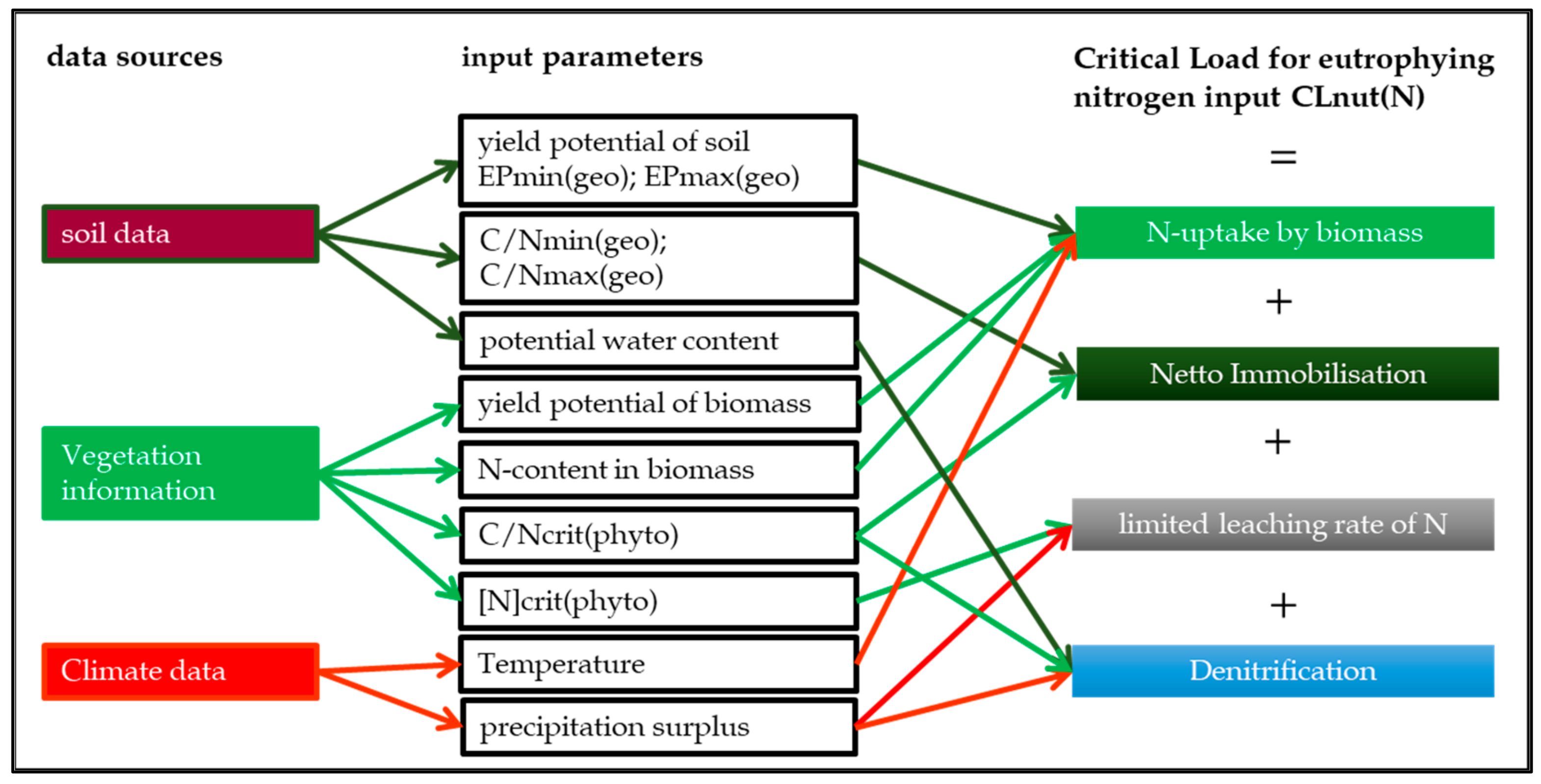
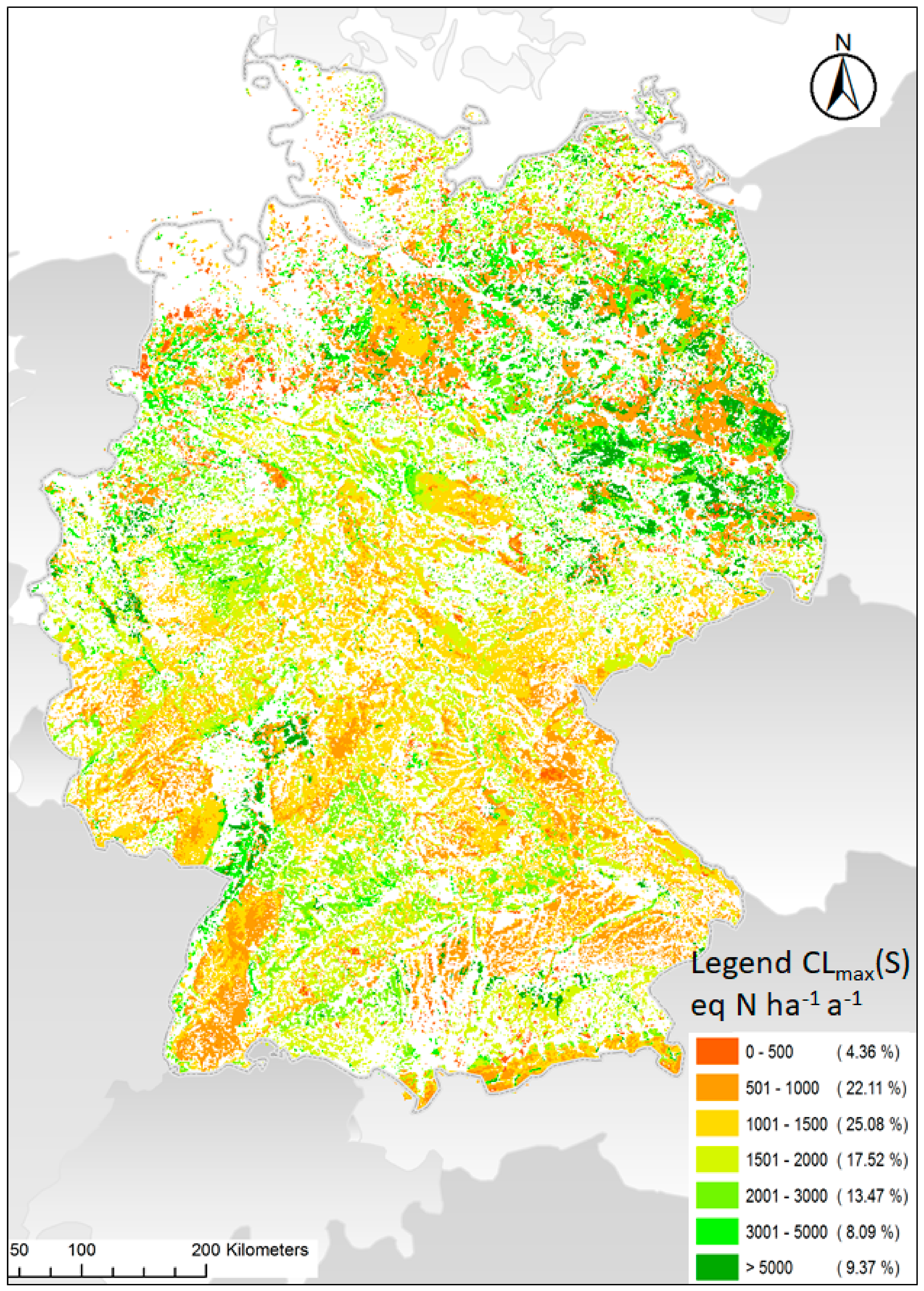
Table 1.
Receptor types and their area shares according to CORINE 2012 [15] in Germany.
Table 1.
Receptor types and their area shares according to CORINE 2012 [15] in Germany.
| CORINE-Code | Description | Area in Germany [ha] | Area in Germany [%] | Proportion of Total Receptors [%] |
|---|---|---|---|---|
| 311 | Deciduous forests | 3,601,128 | 10.05 | 32.05 |
| 312 | Coniferous forests | 55,84,084 | 15.59 | 49.69 |
| 313 | Mixed forests | 1,585,015 | 4.43 | 14.11 |
| 321 | Natural grassland | 187,810 | 0.52 | 1.67 |
| 322 | Heaths and moor heaths | 96,628 | 0.27 | 0.86 |
| 411 | Bogs | 69,595 | 0.19 | 0.62 |
| 412 | Peat bogs | 87,381 | 0.24 | 0.78 |
| 421 | Salt marshes | 25,432 | 0.07 | 0.23 |
| Sum of the receptor areas | 11,237,072 | 31.38 | 100 |
Table 2.
Logarithmic GAPON exchange coefficient Al or H to Ca + Mg + K [eq m−3]−1/2 [18].
Table 2.
Logarithmic GAPON exchange coefficient Al or H to Ca + Mg + K [eq m−3]−1/2 [18].
| Sand | Silt | Clay | Peat | |
|---|---|---|---|---|
| kHBc | 3.296 | 3.193 | 3.616 | 2.809 |
| kAlBc | 0.503 | 0.292 | −0.595 | −0.497 |
Table 3.
Vegetation-dependent critical ratios of basic nutrient cations to aluminum and protons [92].
Table 3.
Vegetation-dependent critical ratios of basic nutrient cations to aluminum and protons [92].
| Vegetation Type | Bc/Alcrit | Bc/Hcrit |
|---|---|---|
| Semi-natural open land vegetation | 0.8 | 0.24 |
| Scots pine, black pine, mountain pine | 1.2 | 1.2 |
| Spruce | 1.2 | 1.2 |
| European larch | 2 | 2 |
| European beech | 0.6 | 0.18 |
| English oak, sessile oak, downy oak | 0.6 | 0.18 |
| Alder, ash | 2 | 1.05 |
| Small-leaved lime, large-leaved lime | 1.4 | 0.42 |
| Hornbeam | 6 | 1.8 |
| Birch, all species | 1 | 0.18 |
| Willow, all species | 0.8 | 0.24 |
| Aspen, poplar | 0.6 | 0.18 |
| Fir | 5 | 1.5 |
| Mountain ash, service tree | 1.4 | 1.4 |
| Downy birch, Carpathian birch | 1 | 1.5 |
| Other deciduous trees | 0.8 | 0.24 |
Table 4.
Ranges of potential net primary productivity (wood and bark) of dominant and sub-dominant tree species [93].
Table 4.
Ranges of potential net primary productivity (wood and bark) of dominant and sub-dominant tree species [93].
| Tree Species | Average Annual Growth Rates after 100 Years (DGZ 100) | |
|---|---|---|
| Net Primary Productivity of Yield Class I | Net Primary Productivity of the Worst Yield Class | |
| Emax(Phyto) | Emin(Phyto) | |
| [t dry mass ha−1 a−1] | [t dry mass ha−1 a−1] | |
| Scots pine | 3.5 | 1.4 |
| Spruce | 4.9 | 3.2 |
| Mountain and Black pine | 0.7 | 0.7 |
| Silver fir | 3.5 | 3 |
| European larch | 2.5 | 2 |
| Beech | 4.9 | 2.4 |
| Oak, all species | 4 | 1.4 |
| Alder | 4.3 | 2.5 |
| Birch, all species | 2.8 | 2.1 |
| Willows, all species | 2.3 | 1.6 |
| Elm, all species | 4.8 | 3 |
| Ash | 3.7 | 2.5 |
| Mountain ash | 2.1 | 1.6 |
| Lime tree, all species | 5.2 | 3 |
| Maple, all species | 3.5 | 2.5 |
| Aspen | 4.5 | 1.1 |
| Hornbeam | 5.6 | 2.5 |
Table 5.
Range of yield potentials (dry matter DM) of the different vegetation types of the forest-free near-natural/semi-natural ecosystems [13].
Table 5.
Range of yield potentials (dry matter DM) of the different vegetation types of the forest-free near-natural/semi-natural ecosystems [13].
| Vegetation Type | Average Annual Growth Rates [t Dry Mass ha−1 a−1] | |
|---|---|---|
| Emin(Phyto) | Emax(Phyto) | |
| Grassland | 0.65 | 1.5 |
| Heathland | 0.7 | 1.5 |
| Dry calcareous grassland | 0.8 | 1.4 |
| Wet and marshy meadows | 0.11 | 1.7 |
| Flood meadows and floodplain meadows | 0.1 | 2.5 |
| Fresh meadows/fresh pastures | 0.8 | 1.6 |
Table 6.
Rules for merging the criteria for the overall classification of soil-specific biomass productivity.
Table 6.
Rules for merging the criteria for the overall classification of soil-specific biomass productivity.
| Subtotal Factor | Criterion |
|---|---|
| Soil water balance | Usable field capacity |
| Porosity with dead water (waterlogging tendency) | |
| Risk of dehydration | |
| Groundwater and backwater influence | |
| Nutrient balance | Cation exchange capacity |
| Usable field capacity | |
| Humus level | |
| Soil structure | Thoroughness |
| Root penetration | |
| Slope of solidification |
Table 7.
Classification and scoring of soils according to pedogenesis and texture with regard to the influence on potential arable wood and grassland yields.
Table 7.
Classification and scoring of soils according to pedogenesis and texture with regard to the influence on potential arable wood and grassland yields.
| Soil Texture According to Pedological Mapping Instructions 5th Edition | Genesis | Porosity < 0.2 µm with Dead Water (pF > 4.2)/Formation of Stagnant Moisture | Risk of Dehydration | Groundwater or Backwater Influence | Usable Field Capacity (Pore Content 0.2–50 µm with Plant-Available Adhesive Water pF 4.2–1.8) | Cation Exchange Capacity | Thoroughness | Root Penetration (Pore Content > 50 µm with Air. pF < 1.8) | Slope of Solidification in the B-Horizon | Relative Yield Potential EP(geo-hoz) |
|---|---|---|---|---|---|---|---|---|---|---|
| Ss | D | 5 | 1 | 1 | 1 | 1 | 3 | 5 | 1 | 2.00 |
| Al | 5 | 1 | 4 | 1 | 1 | 4 | 5 | 1 | 2.36 | |
| K | 5 | 1 | 1 | 1 | 1 | 2 | 5 | 1 | 1.89 | |
| V | 5 | 1 | 1 | 1 | 1 | 2 | 5 | 1 | 1.89 | |
| Su2, Sl2, Sl3, St2 | D | 4 | 2 | 1 | 3 | 2 | 3 | 5 | 1 | 2.67 |
| Al | 4 | 2 | 5 | 3 | 2 | 4 | 5 | 1 | 3.11 | |
| K | 4 | 2 | 4 | 3 | 2 | 3 | 5 | 1 | 2.92 | |
| V | 4 | 2 | 3 | 3 | 2 | 2 | 5 | 1 | 2.72 | |
| Su3, Su4 | D | 3 | 3 | 2 | 4 | 2 | 3 | 5 | 2 | 3.11 |
| Lo | 3 | 3 | 2 | 4 | 2 | 5 | 5 | 2 | 3.33 | |
| Al, K | 3 | 3 | 5 | 4 | 2 | 4 | 5 | 2 | 3.47 | |
| V | 3 | 3 | 3 | 4 | 2 | 2 | 5 | 2 | 3.08 | |
| Vg | 3 | 3 | 1 | 4 | 2 | 1 | 5 | 2 | 2.81 | |
| Slu, Sl4, St3 | D | 3 | 4 | 2 | 5 | 3 | 3 | 4 | 3 | 3.61 |
| Lo | 3 | 4 | 2 | 5 | 3 | 5 | 4 | 3 | 3.83 | |
| Al, K | 3 | 4 | 5 | 5 | 3 | 5 | 4 | 3 | 4.08 | |
| V | 3 | 4 | 3 | 5 | 3 | 2 | 4 | 3 | 3.58 | |
| Vg | 3 | 4 | 1 | 5 | 3 | 1 | 4 | 3 | 3.31 | |
| Ls2-4, Lt2, Lts, Ts4, Ts3 | D | 3 | 4 | 3 | 5 | 4 | 3 | 3 | 4 | 3.86 |
| Lo | 3 | 4 | 2 | 5 | 4 | 5 | 3 | 4 | 4.00 | |
| Al | 3 | 4 | 5 | 5 | 4 | 5 | 3 | 4 | 4.25 | |
| K | 3 | 4 | 4 | 5 | 4 | 3 | 3 | 4 | 3.94 | |
| V | 3 | 4 | 3 | 5 | 4 | 2 | 3 | 4 | 3.75 | |
| Vg | 3 | 4 | 1 | 5 | 4 | 1 | 3 | 4 | 3.47 | |
| Uu, Us, Ut2-4, Uls, Lu | D | 2 | 3 | 3 | 4 | 3 | 3 | 2 | 5 | 3.28 |
| Al | 2 | 5 | 5 | 4 | 4 | 5 | 2 | 5 | 4.00 | |
| Lo | 2 | 3 | 2 | 4 | 4 | 5 | 2 | 5 | 3.58 | |
| K | 2 | 3 | 4 | 4 | 3 | 4 | 2 | 5 | 3.47 | |
| V | 2 | 3 | 3 | 4 | 3 | 2 | 2 | 5 | 3.17 | |
| Vg | 2 | 3 | 1 | 4 | 3 | 1 | 2 | 5 | 2.89 | |
| Lt3, Tu2-4, Ts2, Tl, Tt | D | 1 | 1 | 2 | 3 | 5 | 3 | 1 | 5 | 2.92 |
| Al | 1 | 1 | 5 | 3 | 5 | 4 | 1 | 5 | 3.28 | |
| Lo | 1 | 1 | 2 | 3 | 5 | 5 | 2 | 5 | 3.25 | |
| K | 1 | 1 | 4 | 3 | 5 | 1 | 1 | 5 | 2.86 | |
| V | 1 | 1 | 3 | 3 | 5 | 2 | 1 | 5 | 2.89 | |
| Vg | 1 | 1 | 2 | 3 | 5 | 1 | 1 | 5 | 2.69 | |
| Hh | 1 | 1 | 1 | 1 | 1 | 1 | 1 | 1 | 1.00 | |
| Hn | 1 | 1 | 1 | 2 | 3 | 4 | 3 | 1 | 2.14 |
EP(geo-hor) = Relative yield potential determined by the soil.
Table 8.
Influence of climate/altitude levels and natural balance components on the formation of the plant-available humus level (after [96]).
Table 8.
Influence of climate/altitude levels and natural balance components on the formation of the plant-available humus level (after [96]).
| Soil Texture | Hydromorph | Anhydromorph in Climate/Altitude Zone | With | |||||||
|---|---|---|---|---|---|---|---|---|---|---|
| With Groundwater Influence | With Stagnic Water Influence | Ridge Zone, Higher Mountain Zone | Middle Mountain Zone | Lower Mountains and Hill Country | Lower Mountains and Hill Country | Lowland | Lower Mountains and Hill Country | Lowland | Erosions-Conditional Erosion | |
| All Climate Zones | With Humid Cool Climate | With Moderately Dry Climate | With Dry Warm Climate | |||||||
| Sand | 3 | 3 | 2 | 2 | 4 | 4 | 4 | 4 | 4 | 2 |
| Slightly loamy sand | 4 | 3 | 4 | 4 | 4 | 3 | 4 | 3 | 3 | 4 |
| Silty sand | 4 | 3 | 4 | 4 | 4 | 3 | 3 | 3 | 3 | 4 |
| Strong loamy sand | 4 | 4 | 4 | 4 | 3 | 3 | 3 | 3 | 3 | 3 |
| Clayey loam, sandy clay | 5 | 4 | 3 | 3 | 4 | 3 | 3 | 4 | 4 | 3 |
| Silt, loess | 5 | 4 | 4 | 4 | 3 | 4 | 4 | 3 | 4 | 4 |
| Clay | 5 | 5 | 4 | 4 | 3 | 5 | 5 | 3 | 5 | 5 |
Table 9.
Net substance contents of the main tree species in the dry mass (DM) of derb wood with bark [97,98].
| Species | Ca | Mg | K | N | |
|---|---|---|---|---|---|
| eq t−1 DM | eq t−1 DM | eq t−1 DM | eq t−1 DM | kg t−1 DM | |
| Pine | 53.89 | 19.8 | 16.6 | 77.82 | 1.09 |
| Spruce | 70.36 | 14.8 | 19.7 | 87.10 | 1.22 |
| Copper beech, hornbeam | 89.82 | 21.4 | 35.8 | 103.57 | 1.45 |
| Oaks | 123.3 | 14.8 | 26.9 | 149.93 | 2.10 |
| Alder | 84.83 | 24.7 | 33.3 | 99.95 | 1.40 |
| Birch | 59.88 | 16.5 | 19.2 | 121.37 | 1.70 |
| Mountain pine | 47.9 | 18.1 | 15.6 | 82.14 | 1.15 |
| Willow | 149.7 | 19.8 | 25.6 | 99.95 | 1.40 |
| Other deciduous tree species | 84.83 | 24.7 | 33.3 | 99.95 | 1.40 |
Table 10.
Net substance content in the dry matter (DM) of the above-ground biomass of the forest-free near-natural ecosystems [99,100,101,102,103,104,105,106,107,108,109,110,111,112,113] (5th percentile).
| Vegetation Type of the Open Land | N | Bc (Ca + Mg + K) | |
|---|---|---|---|
| eq t−1 TS | kg t−1 TS | eq t−1 TS | |
| Grassland | 884 | 12.4 | 450 |
| Heathland | 506 | 7.1 | 332 |
| Calcareous dry grasslands | 704 | 9.9 | 743 |
| Wet and marshy meadows | 585 | 8.2 | 371 |
| Flood meadows and floodplain meadows, salt meadows | 1615 | 22.6 | 1286 |
| Fresh meadows/fresh pastures | 983 | 13.8 | 517 |
Table 11.
Statistical distribution of the uptake rate of nitrogen (Nu) and base cations (BCu) into the biomass determined for the German receptor areas.
Table 11.
Statistical distribution of the uptake rate of nitrogen (Nu) and base cations (BCu) into the biomass determined for the German receptor areas.
| Bcu | Nu | |
|---|---|---|
| [eq (Ca + K + Mg) ha−1 a−1] | [kg N ha−1 a−1] | |
| 5th Perc. | 110 | 1.35 |
| 25th Perc. | 217 | 2.76 |
| Median | 276 | 3.33 |
| 75th Perc. | 469 | 4.92 |
| 95th Perc. | 549 | 5.92 |
| Avg. | 329 | 3.9 |
| Soil Parameters | ƒde | |
|---|---|---|
| Gleyed sandy soils | 0.5 | |
| Peaty soils | 0.8 | |
| Podsole | - | 0.1 |
| Drainage status | status excessive | 0 |
| Drainage status | status good | 0.1 |
| Drainage status | status moderate | 0.2 |
| Drainage status | status imperfect | 0.4 |
| Drainage status | status poor | 0.7 |
| Drainage status | status very poor | 0.8 |
| By clay content [%] | <10.5 bis <20.0 | 0.1 |
| By clay content [%] | >20.0 bis <30.0 | 0.2 |
| By clay content [%] | >30.0 bis <37.5 | 0.3 |
| By clay content [%] | >37.5 bis <62.5 | 0.3 |
| By clay content [%] | >62.5 bis >70.0 | 0.5 |
Table 13.
Statistical distribution of the determined denitrification rates (Nde) for the receptor areas in the German critical load dataset.
Table 13.
Statistical distribution of the determined denitrification rates (Nde) for the receptor areas in the German critical load dataset.
| Nde | |
|---|---|
| [kg N ha−1 a−1] | |
| 5th Perc. | 0.08 |
| 25th Perc. | 0.38 |
| Median | 1.08 |
| 75th Perc. | 2.94 |
| 95th Perc. | 10.92 |
| Avg. | 2.57 |
Table 14.
Critical minima and maxima of C/N ratios to ensure a long-term balance of immobilization and mineralization in humus [129].
Table 14.
Critical minima and maxima of C/N ratios to ensure a long-term balance of immobilization and mineralization in humus [129].
| Soil Type of Mineral Topsoil | Minimum C/N Ratio to Ensure Immobilization C/Nmin(geo) | Critical Maximum of C/N Ratio to Ensure Mineralization C/Nmax(geo) |
|---|---|---|
| Raised bog peat | 20 | 60 |
| Rich moor peat | 15 | 40 |
| Large-pored soil types (sand, clay) | 15 | 35 |
| Fine-pored soil types (clay) | 10 | 25 |
| Volcanic soils | 10 | 20 |
| Lime soils | 10 | 20 |
Table 15.
Statistical distribution of the immobilization rates determined for the German receptor areas (Ni).
Table 15.
Statistical distribution of the immobilization rates determined for the German receptor areas (Ni).
| Ni | |
|---|---|
| [kg N ha−1 a−1] | |
| 5th Perc. | 0.65 |
| 25th Perc. | 0.85 |
| Median | 1.05 |
| 75th Perc. | 1.34 |
| 95th Perc. | 2.27 |
| Avg. | 1.20 |
Table 16.
Statistical distribution of the acceptable nitrogen leaching rate (Nle(acc)) determined for the German receptor areas.
Table 16.
Statistical distribution of the acceptable nitrogen leaching rate (Nle(acc)) determined for the German receptor areas.
| Nle(acc) | |
|---|---|
| [kg N ha−1 a−1] | |
| 5th Perc. | 0.12 |
| 25th Perc. | 0.54 |
| Median | 1.68 |
| 75th Perc. | 3.26 |
| 95th Perc. | 10.45 |
| Avg. | 3.06 |
Table 17.
Statistical distribution of the sea salt-corrected deposition rate of base cations (BC*dep).
Table 17.
Statistical distribution of the sea salt-corrected deposition rate of base cations (BC*dep).
| BC*dep = Bcdep | |
|---|---|
| [eq ha−1 a−1] | |
| 5th Perc. | 90 |
| 25th Perc. | 109 |
| Median | 124 |
| 75th Perc. | 142 |
| 95th Perc. | 186 |
| Avg. | 129 |
Table 18.
Allocation of the initial substrates to the substrate classes (authors’ adaptation after [11,139]).
| Parent Material | Class |
|---|---|
| Moor peat | Organic |
| (Fluviatile) sands and thick sandy cover layers | Acidic |
| Sand sols | Acidic |
| Acidic igneous rocks and metamorphic rocks | Acidic |
| Sandstones | Acidic |
| Sediments in the intertidal zone (mudflats) | Intermediate |
| Sand solutes over terrace and gravel deposits | Intermediate |
| Loess and loess derivatives | Intermediate |
| Boulder clay and loam alternating with low-density sandy cover layers | Intermediate |
| Loess over clay substrates | Intermediate |
| Sand loess over loess and loess derivatives | Intermediate |
| Clay substrates | Intermediate |
| Loess over acidic magmatites and metamorphic rocks or sandstone | Intermediate |
| Sandstones, silts | Intermediate |
| Fersiallitic and ferrallitic palaeosols | Intermediate |
| Anthrosol (anthropogenically modified areas) | Intermediate |
| Alluvial sediments | Basic |
| Terrace and gravel deposits | Basic |
| Boulder clay and boulder marls | Basic |
| Silicate substrates | Basic |
| Loess and loess derivatives over basic magmatites and metamorphites | Basic |
| Basic igneous rocks and metamorphic rocks | Basic |
| Bimstuff | Basic |
| Silicate substrates over carbonate substrates (lime and marl substrates) | Basic |
| Alluvial sediments | Calcareous |
| Loess and loess derivatives over carbonate substrates (lime and marl substrates) | Calcareous |
| Carbonate substrates (lime and marl substrates) | Calcareous |
| Carbonate substrates (lime and marl substrates) over clay substrates or loess | Calcareous |
| Claystone | Calcareous |
| Lime marsh | Calcareous |
Table 19.
Matrix for determining the texture class from sand and clay contents (authors’ adaptation after [11,17]).
| Soil Type Clay | Clay Content [%] | Silt Content [%] | Sand Content [%] | Texture Class |
|---|---|---|---|---|
| Ss | 3 | 5 | 92 | 1 |
| Sl2 | 7 | 16 | 77 | 1 |
| Sl3 | 10 | 25 | 65 | 1 |
| Sl4 | 15 | 25 | 60 | 2 |
| Slu | 13 | 45 | 42 | 2 |
| St2 | 11 | 5 | 84 | 1 |
| St3 | 21 | 8 | 71 | 2 |
| Su2 | 3 | 16 | 81 | 1 |
| Su3 | 4 | 33 | 63 | 2 |
| Su4 | 4 | 45 | 51 | 2 |
| Ls2 | 21 | 45 | 34 | 2 |
| Ls3 | 21 | 35 | 44 | 2 |
| Ls4 | 21 | 23 | 56 | 2 |
| Lt2 | 30 | 40 | 30 | 2 |
| Lt3 | 40 | 40 | 20 | 4 |
| Lts | 35 | 23 | 42 | 4 |
| Lu | 24 | 58 | 18 | 3 |
| Uu | 4 | 90 | 6 | 3 |
| Uls | 13 | 58 | 29 | 3 |
| Us | 4 | 65 | 31 | 2 |
| Ut2 | 10 | 87 | 3 | 3 |
| Ut3 | 14 | 75 | 11 | 3 |
| Ut4 | 21 | 70 | 9 | 3 |
| Tt | 75 | 15 | 10 | 5 |
| Tl | 55 | 23 | 22 | 4 |
| Tu2 | 52 | 42 | 6 | 4 |
| Tu3 | 36 | 58 | 6 | 4 |
| Tu4 | 28 | 69 | 3 | 3 |
| Ts2 | 55 | 8 | 37 | 4 |
| Ts3 | 40 | 8 | 52 | 4 |
| Ts4 | 30 | 8 | 62 | 2 |
Soil texture classes: Hh = Raised bog; Hn = Fen; Ls2–4 = Weak to strong sandy loam; Lt2 = Weak clayey loam; Lt3 = Medium clayey loam; Lts = Sandy–clayey loam; Lu = Silty loam; Sl2 = Light loamy sand; Sl3 = Medium clayey sand; Sl4 = Very loamy sand; Slu = Silty–clayey sand; Ss = Pure sand; St2 = Light clayey sand; St3 = Medium clayey sand; Su2 = Light silty sand; Su3 = Medium silty sand; Su4 = Strongly silty sand; Tl = Clayey clay; Ts2 = Slightly sandy clay; Ts3 = Medium sandy clay; Ts4 = Very sandy clay; Tt = Pure clay; Tu2–4 = Weak to strong silty clay; Uls = Sandy–clayey silt; Us = Sandy silt; Ut2–4 = Weak to strong clayey silt; Uu = Pure silt.
Table 20.
Matrix for determining the weathering class (WRc) from the substrate and texture class [11].
Table 20.
Matrix for determining the weathering class (WRc) from the substrate and texture class [11].
| Weathering Rate Classes | Texture Class | ||||
|---|---|---|---|---|---|
| Parent Material | 1 | 2 | 3 | 4 | 5 |
| Acidic | 1 | 3 | 3 | 6 | 6 |
| Intermediate | 2 | 4 | 4 | 6 | 6 |
| Basic | 2 | 5 | 5 | 6 | 6 |
| Calcareous | 20 | ||||
| Organic | W(class) = 6 for basic peats, otherwise Wc(class) = 1 | ||||
Table 21.
Statistical distribution of the determined release rate of base cations through weathering (BCw).
Table 21.
Statistical distribution of the determined release rate of base cations through weathering (BCw).
| BCw | |
|---|---|
| [eq (Ca + K + Mg + Na) ha−1 a−1] | |
| 5th Perc. | 295 |
| 25th Perc. | 870 |
| Median | 1297 |
| 75th Perc. | 1916 |
| 95th Perc. | 4267 |
| Avg. | 1579 |
Table 22.
Share of receptor areas in Germany in the classes of critical loads for eutrophying nitrogen inputs.
Table 22.
Share of receptor areas in Germany in the classes of critical loads for eutrophying nitrogen inputs.
| CLnut(N) Class | Receptor Area Share |
|---|---|
| kg N ha−1 a−1 | % |
| <5 | 20.16 |
| 5–<10 | 33.87 |
| 10–<15 | 22.68 |
| >15 | 22.95 |
Table 23.
Share of receptor areas in Germany in the classes of critical loads for acidifying sulphur inputs.
Table 23.
Share of receptor areas in Germany in the classes of critical loads for acidifying sulphur inputs.
| CLmax(S) Class | Receptor Area Share |
|---|---|
| eq ha−1 a−1 | % |
| <500 | 4.36 |
| 501–1000 | 22.11 |
| 1001–1500 | 25.08 |
| 1501–2000 | 17.52 |
| 2001–5000 | 8.09 |
| >5000 | 9.37 |
Table 24.
Comparison of the CLnut(N)-ranges according to different methods.
| EUNISCode | SMB CLnut(N) min [14] | SMB CLnut(N) av. [14] | SMB CLnut(N) max [14] | CLemp 2022 [12] | Reliability 2022 * [12] |
|---|---|---|---|---|---|
| kg N ha−1 a−1 | |||||
| MA2243 | 16 | 26 | 33 | 10–20 | (#) |
| Q11111 | 4 | 8 | 22 | 5–10 | ## |
| Q222 | 6 | 8 | 11 | 5–15 | ## |
| Q412 | 10 | 15 | 32 | 15–25 | # |
| Q4221 | 6 | 16 | 27 | 15–25 | # |
| Q433 | 13 | 31 | 79 | 15–25 | # |
| R1A3 | 10 | 33 | 69 | 10–20 | ## |
| R1M2 | 2 | 15 | 26 | 6–10 | ## |
| R1P | 1 | 9 | 19 | 5–15 | (#) |
| R1Q | 11 | 12 | 14 | 5–15 | (#) |
| R222 | 10 | 35 | 89 | 10–20 | (#) |
| R231 | 9 | 16 | 53 | 10–15 | # |
| R351 | 22 | 34 | 46 | 15–25 | (#) |
| R372 | 7 | 9 | 15 | 10–20 | # |
| R44311 | 7 | 27 | 56 | 5–10 | # |
| S223 | 1 | 6 | 11 | 5–10 | # |
| S422 | 7 | 8 | 13 | 5–15 | ## |
| T171 | 6 | 18 | 63 | 10–15 | (#) |
| T181 | 5 | 17 | 48 | 10–15 | (#) |
| T1B1 | 6 | 13 | 18 | 10–15 | (#) |
| T1E16 | 7 | 13 | 31 | 15–20 | (#) |
| T312 | 3 | 12 | 48 | 10–15 | (#) |
| T323 | 4 | 10 | 19 | 10–15 | (#) |
| T35211 | 3 | 9 | 45 | 5–15 | # |
* ## reliable; # quite reliable and (#) expert judgement.
Table 25.
Comparison of the critical loads and critical limits calculated according to SMB from the Mapping Manual [11,14] with those including vegetation-specific limits derived from the BERN model by the authors.
| CL Class | CLmax(S)(Manual) | CLmax(S)(BERN) |
|---|---|---|
| eq S ha−1 a−1 | % of the Receptor Area | |
| <500 | 7.93 | 4.36 |
| 500–1000 | 41.15 | 22.11 |
| 1000–1500 | 18.49 | 25.08 |
| 1500–2000 | 14.23 | 17.52 |
| 2000–3000 | 10.2 | 13.47 |
| 3000–>5000 | 7.99 | 17.46 |
| CL class | CLnut(N)(Manual) | CLnut(N)(BERN) |
| kg N ha−1 a−1 | % of the Receptor Area | |
| <5 | 19.0 | 20.16 |
| 5.0–10.0 | 30.98 | 33.87 |
| >10.0–15.0 | 18.51 | 22.68 |
| >15.0 | 31.51 | 22.95 |
Disclaimer/Publisher’s Note: The statements, opinions and data contained in all publications are solely those of the individual author(s) and contributor(s) and not of MDPI and/or the editor(s). MDPI and/or the editor(s) disclaim responsibility for any injury to people or property resulting from any ideas, methods, instructions or products referred to in the content. |
© 2023 by the authors. Licensee MDPI, Basel, Switzerland. This article is an open access article distributed under the terms and conditions of the Creative Commons Attribution (CC BY) license (https://creativecommons.org/licenses/by/4.0/).
Share and Cite
MDPI and ACS Style
Schlutow, A.; Scheuschner, T. Determination of Critical Loads for Eutrophying and Acidifying Air Pollutant Inputs for the Protection of Near-Natural Ecosystems in Germany. Atmosphere 2023, 14, 383. https://doi.org/10.3390/atmos14020383
AMA Style
Schlutow A, Scheuschner T. Determination of Critical Loads for Eutrophying and Acidifying Air Pollutant Inputs for the Protection of Near-Natural Ecosystems in Germany. Atmosphere. 2023; 14(2):383. https://doi.org/10.3390/atmos14020383
Chicago/Turabian StyleSchlutow, Angela, and Thomas Scheuschner. 2023. "Determination of Critical Loads for Eutrophying and Acidifying Air Pollutant Inputs for the Protection of Near-Natural Ecosystems in Germany" Atmosphere 14, no. 2: 383. https://doi.org/10.3390/atmos14020383
Note that from the first issue of 2016, this journal uses article numbers instead of page numbers. See further details here.