Unraveling the Regional Specificities of Malbec Wines from Mendoza, Argentina, and from Northern California

Abstract

This study explores the relationships between chemical and sensory characteristics of wines in connection with their regions of production. The objective is to identify whether such characteristics are significant enough to serve as signatures of a terroir for wines, thereby supporting the concept of regionality. We argue that the relationships between characteristics and regions of production for the set of wines under study are rendered complicated by possible non-linear relationships between the characteristics themselves. Consequently, we propose a new approach for performing the analysis of the wine data that relies on these relationships instead of trying to circumvent them. This new approach follows two steps: We first cluster the measurements for each characteristic (chemical, or sensory) independently. We then assign a distance between two features to be the mutual entropy of the clustering results they generate. The set of characteristics is then clustered using this distance measure. The result of this clustering is a set of sub-groups of characteristics, such that two characteristics in the same group carry similar, i.e., synergetic information with respect to the wines under study. Those wines are then analyzed separately on the different sub groups of features. We have used this method to analyze the similarities and differences between Malbec wines from Argentina and California, as well as the similarities and differences between sub-regions of those two main wine producing countries. We report detection of groups of features that characterize the origins of the different wines included in the study. We note stronger evidence of regionality for Argentinian Malbec wines than for Californian wines, at least for the sub regions of production included in this study.

1. Introduction

Malbec (Vitis vinifera L. cv. Malbec) is a red grape variety with origins in France, where its culture persists in the Cahors and Bordeaux regions. Its characteristic “inky” dark color and robust tannins make it one of the six red grape varieties allowed in the blending of red Bordeaux wines. After a severe frost event, however, that wiped out the majority of the Malbec vineyards in the area of Bordeaux in 1956 [1], it became less popular in that region, considered to be too sensitive to the weather, causing the grapes not to produce a quality wine. It remains more popular and probably better suited in and around Cahors, where it is still a main component of the blends of that region. French single variety Malbec wines are a more recent phenomenon due in part to the international recognition of Malbec.

Malbec is a frail variety of grapes, demanding specific ecological conditions and vineyard management techniques. It does not reach the development of its varietal characteristics in all regions. It requires large night-day temperature variations, with cool nights. Maximum mean day temperatures should not be higher than 30 °C during the ripening months [2]. Such conditions are met in the high altitude regions of Mendoza, Argentina, such as in the Luján de Cuyo and the Uco Valley in the foothills of the Andes mountains. Malbec grapes were introduced in and around Mendoza by French agricultural engineers as early as in the mid-nineteenth century. Since then, they have greatly contributed to the success of the Mendoza province as a wine region [3]. A relatively more recent surge in the production and popularity of varietal Malbec wine was also seen in California, USA, at the beginning of the 21st century [4]. The total production of Malbec wines in the US, of which around 85% come from California, remains however small, representing less than 3% of the production of Malbec wines in Argentina. This should be compared with the import of Argentinian Malbec wines in the US, which has enjoyed an almost exponential growth between 2000 and 2009: from 0.05 to 1.4 million cases [5].

In contrast to the geographic situations of Malbec vineyards in Argentina, most Californian Malbec vineyards are located in low altitude regions, including the Napa and Sonoma Valleys and other neighboring regions. Such differences in altitude and concomitant climate conditions between Mendoza, Argentina and Northern California, USA are expected to bestow distinct regionality, or “terroir” upon the resulting wines. This concept of regionality is of significance both for the consumers and the wine makers. It is well known, for example, that the region of origin is an important decision-making factor used by (knowledgeable) wine consumers when purchasing wine [6], assuming differences between regions even for wines made from the same type of grapes. It is often unclear, however, how the decision is made. Wine makers are even more concerned, as regionality, or lack of regionality, influences how wines are made. In parallel, while large producers buy grapes coming from a large geographic area to increase production, thereby refuting the concept of regionality, more local producers emphasize the concept of, and importance of, a terroir as it provides a signature and specificity to their own production. This study takes an analytical approach to measuring the importance of such regional specificity using chemical and sensory data for two types of Malbec wines, from Argentina and California.

There have been numerous studies characterizing regional differences in wines, including Cabernet Sauvignon from Australia [7] and from France [8], and Moravia Agria from Spain [9], to only list a few. A much smaller number of studies have compared the sensory profiles of wines from multiple countries, including red wines from Australia and China [10], and Sauvignon Blanc wines from France, New Zealand, Spain, South Africa, and the United States [11]. The regionality of Malbec wines has been studied based on their phenolic compositions [12,13,14] and elemental composition from soils to determine wine provenance in Argentina [15,16]. Two studies have investigated regional sensory differences of Malbec wines from Argentina. Goldner and Zamora [2] analyzed 56 “non-commercial” Malbec wines (i.e., those wines were tank sampled, did not have contacts with oak, with no malolactic fermentation) from seven viticultural regions in Argentina. They found clear sensory differences among the Malbec wines produced in the different regions. Aruani et al. [17] investigated the regional characteristics of 32 commercial Malbec wines from eight Argentinean wine regions. All those wines were tank-fermented with no oak aging. Similar to the Goldner and Zamora findings, the study by Aruani et al. showed significant sensory differences among the Malbec wines, with some of the wine regions grouped as they are geographically close or share similar climatic conditions. Three more recent studies have compared the characteristics of Malbec wines from California, USA, and Mendoza, Argentina. Buscema and Boulton [18] compared Malbec wines using chemometrics on 33 phenolic components comprising individual anthocyanins, low molecular weight phenolics, and total phenolics. They showed that Malbec wines produced in Mendoza have clearly different phenolic profiles than those produced in California. Using Plasma atomic emission spectroscopy, Nelson et al. [19] showed that the Malbec wines from Argentina and from the United States were clearly separated based on their elemental profiles, using only six elements, Sr, Rb, Ca, K, Na, and Mg. Using both chemical and sensory profiles, King et al. [20] also highlighted differences between Argentinian and Californian Malbec wines. They found that Malbec wines from Mendoza had riper fruit, sweetness, and higher alcohol levels, while the Californian Malbec wines had more artificial fruit and citrus aromas, and bitter taste. The compositional differences between the two countries were found to be related more to altitude differences than to precipitation and growing degree days.

Two types of data analyses were primarily performed in the studies of regionality mentioned above, namely Analysis of Variance (ANOVA) and Principal Component Analysis (PCA), see for example Buscema and Boulton [18]. In this paper, we argue that it can be difficult to derive insight from such analyses. ANOVA, for example, is a single feature-based approach. Wine characteristics (both chemical and sensory), however, are expected to be dependent, making it difficult to analyze them independently. In addition, this dependency is likely to be non-linear, especially as we combine chemical with sensory data, making it difficult to interpret based on the linear combination of features imposed by the PCA. We propose instead a more exploratory data-driven approach to relate wine features with regionality that is based on the following ideas. First, as briefly mentioned above, we note that the features that characterize wines should they be chemical data or sensory profiles, are expected to be at least weakly dependent to each other. The existence of such dependencies can be captured as a network among the features. A network is likely to contain communities. Each community is then expected to capture a physical mechanism. We then apply a method for identifying such network between the features, for detecting communities within that network (termed ”synergistic feature-groups”). Finally, we analyze the relationships between the wine features and the regions those wines are coming from (the “response variables”) using those communities as a framework. We note that this method is related to the concept of feature selection [21], although it expands upon selection as it attempts to identify communities within features, rather than selecting one group of those features. The whole procedure is derived from previous work from the authors [22,23,24,25,26].

The paper is organized as follows. First, we provide a brief description of the data used to analyze different wines from California, USA, and Mendoza, Argentina. The following section includes a comprehensive description of our method for studying wine regionality. In the Result section, we analyze the similarities and differences between wines from Mendoza and California, as well as the similarities and differences between sub-regions of those two main regions. We conclude the paper with a discussion on possible improvements and extensions of our method.

2. Materials

We note first that all the data considered in this study have been published before. Readers are referred to King et al. [20] and Buscema and Bolton [18] for detailed information. Here, we provide only a brief description of those data for the sake of clarity.

Forty-one different Malbec wines were evaluated in this study, made from fruit originating from 41 different viticultural sites, 26 in Argentina, and 15 in California. All wines were made in the 2011 vintage in fermentation triplicates. The chemical components and the tasting properties of each of the replicates are then studied in triplicate (i.e., three independent measures are taken).

In the Mendoza province in Argentina, 26 viticultural sites were chosen from four wine regions: Luján de Cuyo (referred to as Luján), Maipú, Tupungato and San Carlos. The latter two regions are within the Uco Valley. An additional 15 viticultural sites were chosen within California, USA from five wine regions: Lodi, Monterey, Napa, Sonoma and Yolo County. A full description of those sites is provided in Table 1 of King et al. [20].

All wines were analyzed for four standard chemical parameters (titratable acidity (TA), pH, volatile acidity (VA) and ethanol (EtOH)), as well as 48 volatile compounds expected in red wines by standard published methods. We note that Benzyl-Alcohol was only sufficiently detected within California wines, but not Argentinian samples. Accordingly, 51 chemical measurements (47 volatile compounds and 4 standard parameters) are shared between the California and Argentina Malbec wines. When Californian wines are analyzed separately, 52 measurements are considered due to the inclusion of Benzyl-Alcohol measurements. Sensory descriptive analysis was undertaken in two separate panels, each of which was run within half a year of the respective harvest. Several panelists participated in both studies. While both panels decided on 23 sensory attributes to describe the respective wines, only 18 of these sensory features are shared between both the Argentinian and Californian wines. Accordingly, 69 features will be considered when comparing wines from both countries, while the original sets of features will be considered when analyzing each country separately. For more details, interested readers are referred to King et al. [20] for tables of volatile compounds or sensory attributes.

As often found in experimental settings, some of the data are missing. As each measure (chemical data or sensory data) are provided in triplicate (i.e., as the results of three independent measurements), we implemented the following procedure to handle those missing values. If at least one of the three values for a feature is known, the missing value (s) is (are) taken to be the average of the known value (s). If all three values are not known, we build for that specific feature a multilinear regression model based on all the wines for which this feature is known. The same regression model is used for all three missing values, which are then set to be identical.

All those data are available at http://web.cs.ucdavis.edu/~koehl/Projects/index.html.

3. Methods

3.1. Motivation and Algorithm

As in any scientific setting, a computational experiment is designed to provide insight into the relationships between the parameters that define the objects in a system and the observations that are made in order to understand this system. In the language of data analysis, the objects correspond to labeled subjects contained in a subject space. The parameters are labels that form the response feature space; they are linked to their corresponding observations that form the covariate feature space. The main objective of data analysis is then to gain insight into the relationships between the covariate features and the response features. These relationships can then be used to making predictive inferences about unlabeled covariate data.

In the setting considered here, the subject space is a set of N different Malbec wines that come from different areas of either the Mendoza region in Argentina, or the Northern California region in the United States. The covariate features correspond to a set of chemical measurements and a set of sensory evaluations of the wines. This information is stored in a data matrix D such that D (i,j) is the value for measurement j (that can be chemical or sensory) on wine i. In addition, we know the provenance of each of the N wines. This labeling of regional and sub-regional information is stored and arranged into a Nx1 response vector R such that R (i) is a label defining the region (Mendoza or California) and sub-region (the specific valley in the corresponding region) in which wine i was produced. Our goal is to identify associative patterns between features and responses that allow us to define signature for each wine region, namely characterize the regionality of each wine. The main difficulties relate to complex correlations between features, as those may reveal different physical processes bound to wine making. To circumvent these problems, we align our approach with the concept of feature selection, or more specifically feature organization, whose goal is to identify groups of associated features, which we refer to a group of synergistic features, analyze the patterns between wines and features for each of those groups separately, and finally analyze the patterns within the resulting heat maps contingent on the response vector. The complete procedure includes four main steps, namely:

Step 1.

Normalize and generate a digital coding for each of the feature j characterizing the N wines.

Step 2.

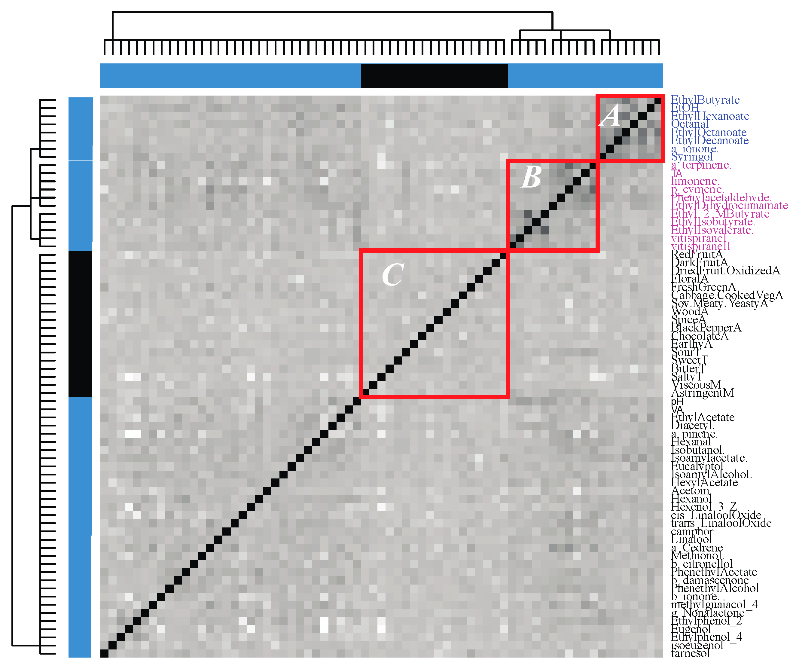
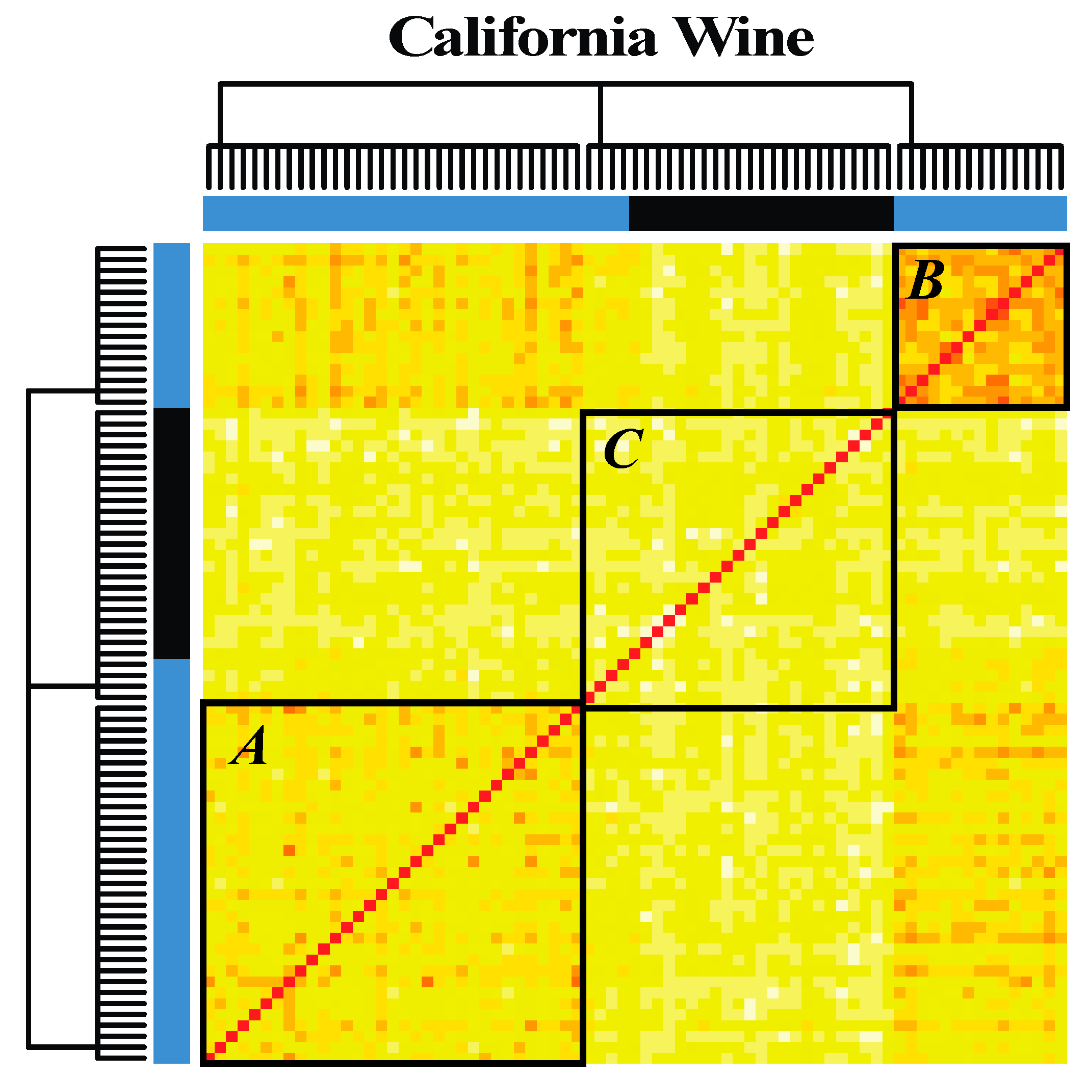
Compute a mutual entropy E (j,k) between any pair of features j and k. Set this entropy measure to be a distance on the feature space, and use this distance to construct a DCG tree on the features. The clusters identified on the DCG tree form the different groups of synergistic features.

Step 3.

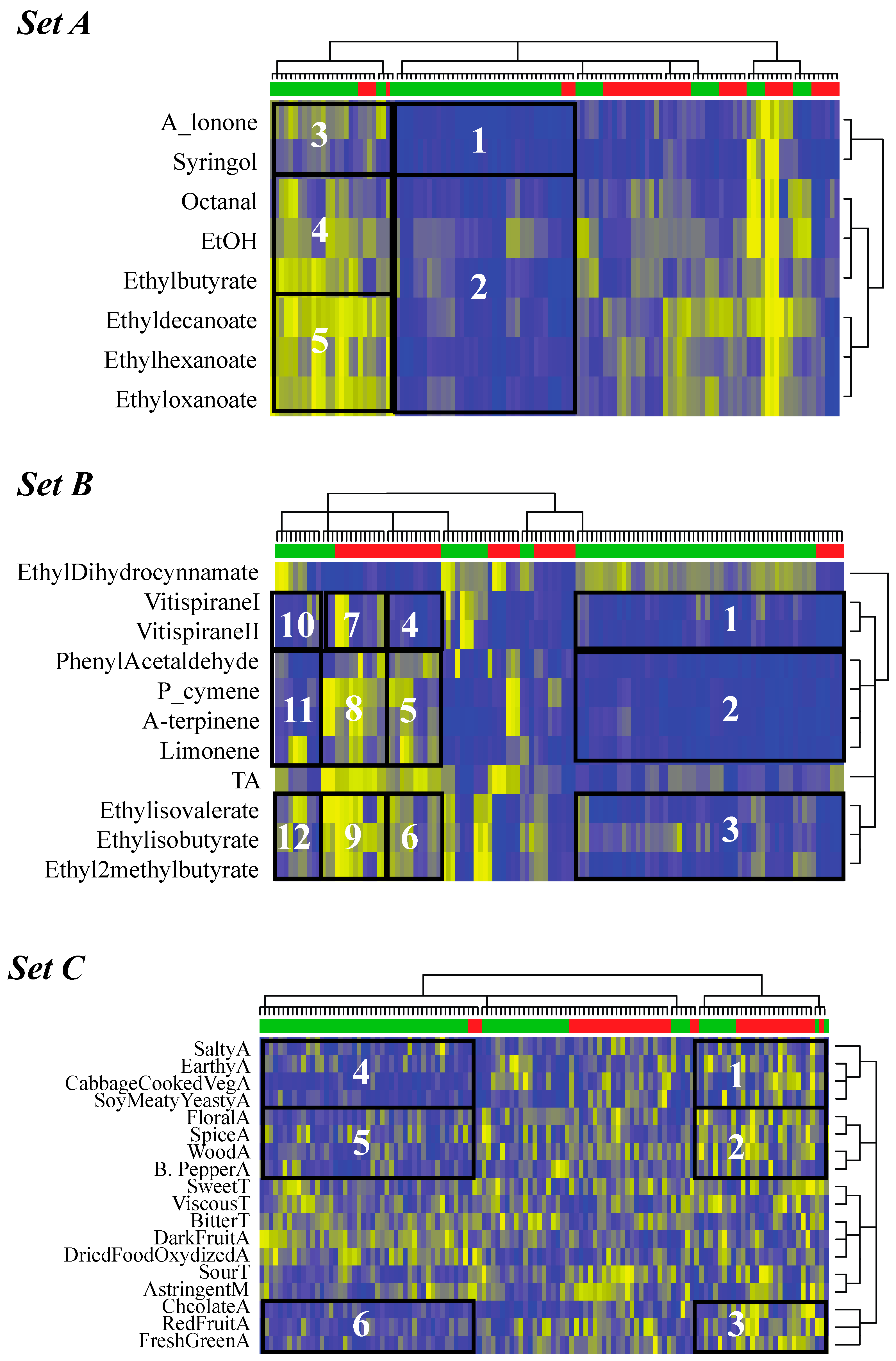
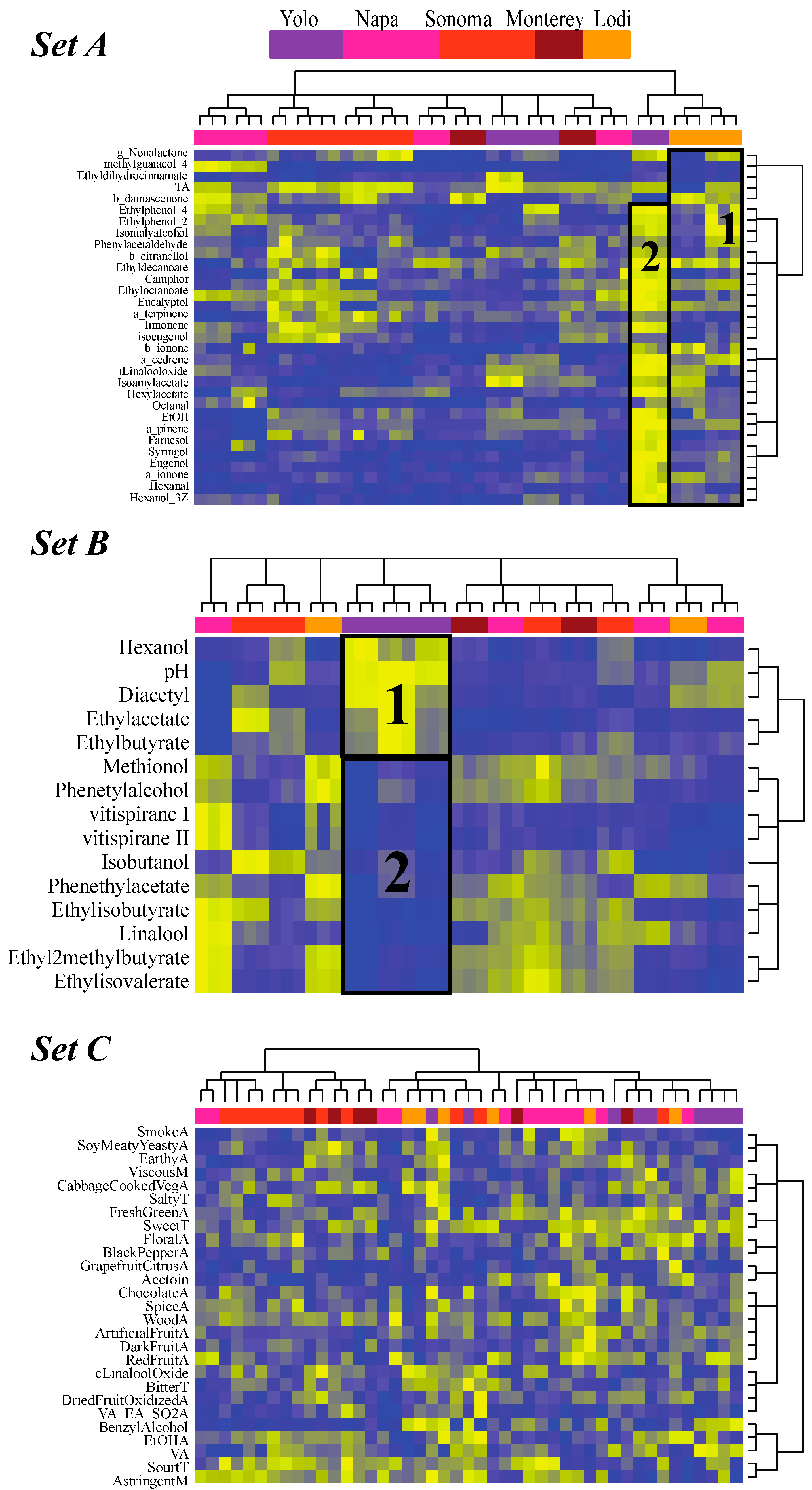
Restrict the data matrix D by only keeping the features corresponding to one of the groups identified in step 2. Perform Data Mechanics on this restricted matrix, and build the corresponding heat map. Repeat this procedure for all groups of features from step 2.

Step 4.

For each heat map generated in step 3, analyze the clusters of wine identified by the Data Mechanics procedure, contingent to their response values (i.e., region information). For those clusters with high content of wines that have the same response value, analyze the corresponding patterns among the features. Repeat the procedure for all heat maps from step 3.

The different steps of this procedure are described in more details in the following subsections.

3.2. Step 1: Normalization and Digital-coding of the Individual Features

Full descriptions of the procedure used in this step are available in the Supplemental material of Fushing et al. [25] and in [27]. Here, we provide the general ideas behind this procedure, to ensure completeness of the description of our method, and for sake of clarity.

Digital coding is the process of associating a number, or digital code, to objects characterized by numerical values such that “similar” objects share the same code. A simple way to perform encoding would be to sort the numerical values that define the objects, break them into groups, and assign to each object the index of the group it belongs to. This naive way to perform encoding is however difficult to implement: finding the right number of groups as well as finding where, and how to separate the values into groups are tasks that are ill-defined, as there are no underlying universal rules that define them. We use a different approach in which we learn the definitions of the groups from the data.

Let us consider a feature j charactering the wines considered here. The values for that feature for all N wines form a set of N data points $x_i, i \in \left[1, N\right]$. We first normalize these data points, i.e., we define ${\tilde{x}}_i=\frac{x_i-\overline{x}}{\sigma }$ where $\overline{x}$ and $\sigma$ are the mean value and standard deviation of all N values x_i, respectively. The cumulative distribution function (CDF) for the normalized values $\tilde{x}$ usually follows a sigmoid-like curve, with changes in the slope of the curve that matches with changes in the similarities of the data. That is, by fitting a possibly gapped piecewise linear function onto the CDF, it is possible to reveal the positions of those changes. Each line segment on the CDF covers a subset of the data points. The corresponding region in the distribution is more or less uniformly distributed, and therefore corresponds to a horizontal density. The collection of those horizontal pieces of density distribution represents a histogram. Gaps in the piecewise linear function approximation appear as gaps (i.e., blank bars) in the histogram representation of the data.

However, one major computing difficulty in the method described above remains: the set L of all gapped piecewise linear functions that can approximate the CDF of the normalized data points is much too large to be explored systematically. We let the data solve this problem in an unsupervised manner. We use the hierarchical clustering (HC) algorithm to cluster the normalized data points, using the Euclidean distance as an empirical distance measure on these points. HC algorithm generates a tree on the data. Each level on this tree corresponds to a partition of the N ordered data points through a collection of tree branches, say P, and each of these branches is then taken to correspond to a line segment. A gap is identified when two consecutive line segments do not share an internal node in the tree. The corresponding histogram contains P bins, that may, or may not be separated by gaps. This parameter P is chosen to provide balance between decoding errors and coding lengths of all bins’ boundaries. Points that belong to the same bin in the histogram are given the same code. Two consecutive bins are given consecutive codes, unless they are separated by a gap, in which case a gap is set in the coding.

There are two sets of parameters in the procedure described above: the number of clusters P in the hierarchical tree, and the gaps in coding associated with gaps between bins. Those parameters were set heuristically. We first generated all HC trees for all features describing the wines considered in this study. Based on those trees, we decided on P to be 4. We note that for some of the trees, there are no cuts that correspond to 4 clusters; for those trees, we picked P that is closest to 4. All histograms were then coded to cover the whole range [1,M] with M set to 10, and the gaps in the coding were adjusted to yield the largest linear correlation between the distances between the bins, and the distances between the codes assigned to the bins.

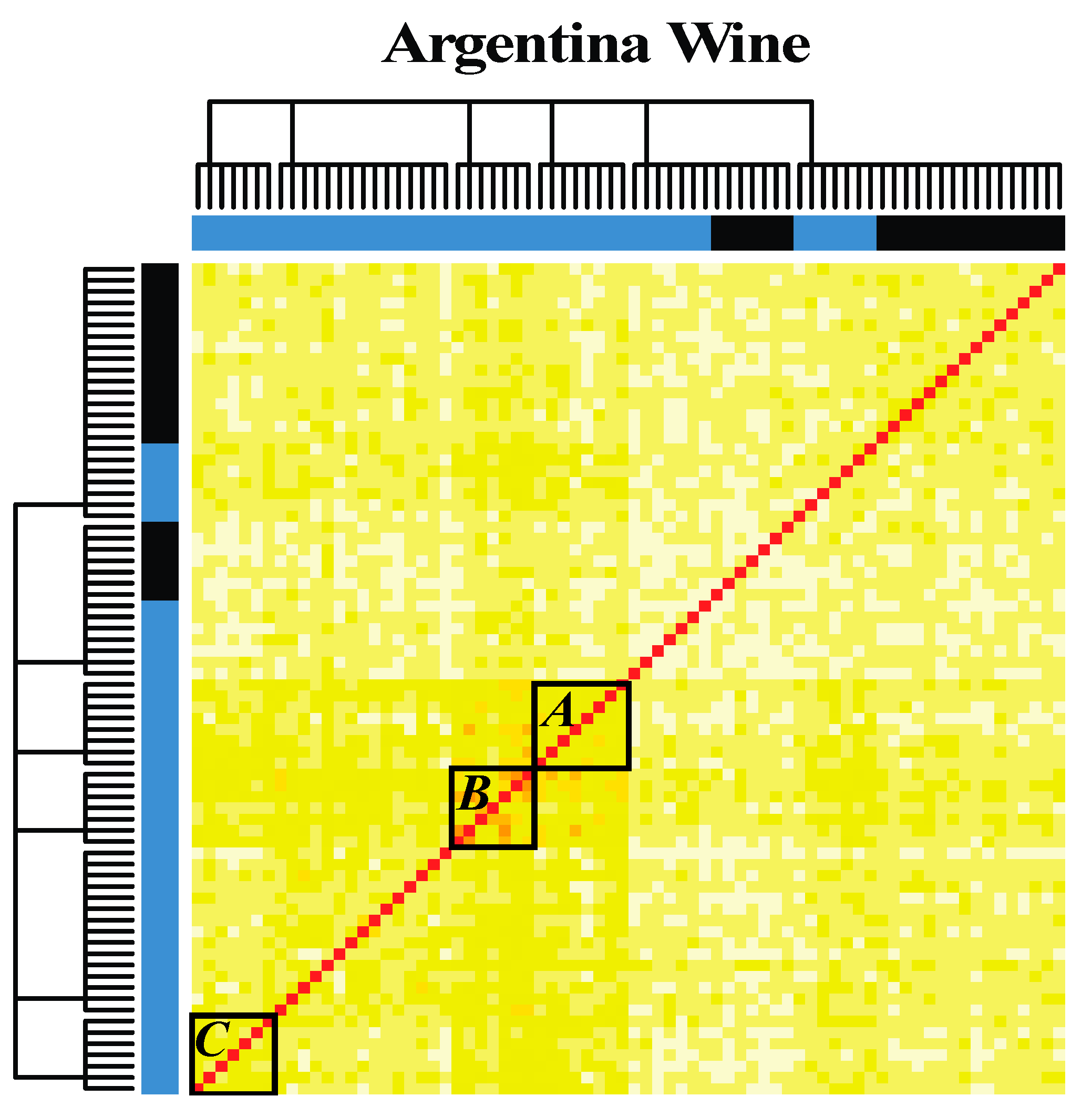
3.3. Step 2: Identification of the Groups of Synergistic Features

For a comprehensive description of this step, including a presentation of mutual entropy, we refer the reader to Fushing et al. [26]. We note that entropy is a quantitative measure of “disorder”, or randomness of a thermodynamic system. From an information theory point of view, entropy is the amount of information in a message. When comparing two variables, entropy can be seen as a measure of the similarity or association of those variables, with a low value meaning that the variables are similar.

Briefly, let us consider two features j and k, whose values over the N wines have been digitally coded in the range [1,M] according to Step 1 defined above. We evaluate how different those two categorizations of the wines are, using the idea of (conditional) mutual entropy. The coding based on features j and k leads to partitioning of the N wines into two distinct groups of M sets, $C=\left\{C_1, C_2,\dots ,C_M\right\}$, and $D=\left\{D_1, D_2,\dots ,D_M\right\},$ respectively. Let us consider one of the sets of C, say $C_{\alpha }$, where $\alpha \in \left[1,M\right]$. This set may contain elements of each of the partitions $D_{\beta }$, with $\beta \in \left[1, \mathrm{M}\right]$. The Shannon entropy of the set $C_{\alpha }$ is defined as:

$$E\left(C_{\alpha }/D\right)=-{\displaystyle \sum }_{\beta =1}^M\frac{\left|C_{\alpha }\cap D_{\beta }\right|}{\left|C_{\alpha }\right|}\log \left(\frac{\left|C_{\alpha }\cap D_{\beta }\right|}{\left|C_{\alpha }\right|}\right)$$

(1)

where |A| means the cardinality of set A. This entropy measures how much the composition of the set $C_{\alpha }$ differs from a composition that would be obtained from a random sampling based on the partitioning defined by D.

The conditional entropy of the partitioning C with respect to the partitioning D is then given by:

$$E\left(C/D\right)={\displaystyle \sum }_{\alpha =1}^M\frac{\left|C_{\alpha }\right|}{N}E\left(C_{\alpha }/D\right)$$

(2)

We can define in a similar manner the conditional entropy of the partitioning D given the partitioning C. Based on those two conditional entropies, we defined the mutual entropy of the features j and k:

$$E\left(i,j\right)=\frac{E(C/D)+E(D/C)}{2}$$

(3)

Two features j and k whose mutual entropy E(j,k) is low are called synergistic. It should be noted that such synergistic features may not necessarily be linearly correlated. Using this mutual entropy as a distance measure, it is then possible to cluster the features. We use the Data Cloud Geometry (DCG) method for that purpose. A full description of DCG method and algorithm is provided in the original papers [22,23]. We provide a brief outline below for sake of completeness.

Starting from a set of data points (here, the set of features characterizing the wines) and an empirical measure d that defines the distances between these data points (the mutual entropy defined above), the goal is to derive a multi-scale partitioning of these data that illustrates their geometry. The main idea of the DCG method is to identify this geometry with a potential landscape; this is done based on two key observations. Firstly, it is observed that the empirical distance measure d imposes a weighted graph onto the collection of data points. By equating the weight on an edge to the difference of potential between the two nodes it connects, with a “temperature” as a parameter, this weighted graph is seen as equivalent to a potential landscape, typically characterized by many wells with various depths. Secondly, it is possible to explore this landscape using a Monte Carlo approach; by studying this landscape at different temperatures, the DCG procedure extracts the geometric structure of the data. This geometric structure can then be summarized as a hierarchical tree, the DCG-tree [23].

The DCG method is designed to replace the empirical distance measure with an effective ultrametric distance that reflects the underlying structure of the data. An ultrametric space satisfies a strong triangular inequality, namely $d\left(x,y\right)\le \max \left(d\left(x,z\right),d\left(y,z\right)\right)$, for any three points {x,y,z} in that space. An important consequence of this inequality is that any such triplet of points forms an isosceles triangle, that is, any three points determine at most two distances. While such a property is counterintuitive with respect to our usual understanding of distances between points, it is readily amenable to a tree representation of the underlying space. Such a ultrametric tree representation is in fact valid for any ultrametric space. It has the important property that the ultrametric distance between two data points is exactly equal to the sum of the lengths of the branches in the tree that connect the two points (additivity property). This property does not always carry over for a distance measure that only satisfies the triangular inequality. We note also that in such a tree representation, any node can contain more than two child branches due to “equal” distances, where equal can be interpreted as not having enough information about those children nodes to sustain further separation among them. The tree representation therefore provides a hierarchical organization of the features that can be used to assess the interdependences between those features.

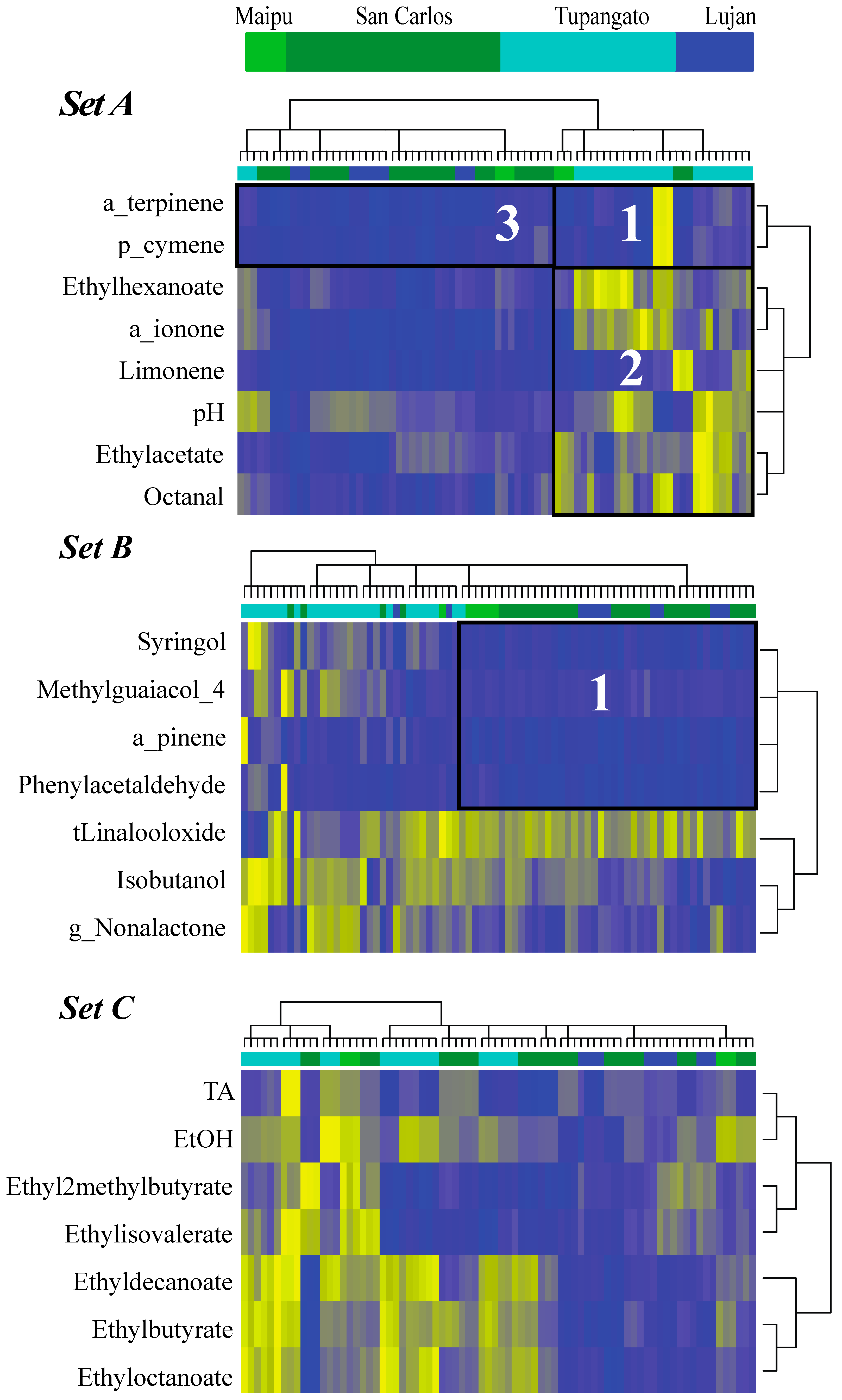
3.4. Step 3: Analyzing Patterns between Wines and Features Using Data Mechanics

Let us consider one set of P synergistic features found in Step 2 described above. We restrict the full data matrix D onto this set of features. This gives us a new data matrix, D_c, whose rows are the N wines and columns the P selected features. As we are going to compare the values of those features, we first transform each of them separately using a linear transform, such that their values are in the range [0,1]. In general, neither the wines along the row axis of D_c nor the features along the column axis of D_c are ordered with respect to temporal, spatial or ordinal axes of any kind. Consequently, direct visualization of the normalized data matrix D_c will provide little information about its “geometry”, i.e., about the patterns it contains. We have recently proposed a data-driven approach to unravel the geometry of such a matrix, referred to as Data Mechanics [24,25], which we propose to use in the context of analyzing the regionality of wines. Data Mechanics works by re-organizing the rows and columns of the data matrix through permutations, regrouping them based on similarity. It proceeds by iteratively computing two tightly coupled ultrametric trees onto the row and columns, where “coupling” refers to the concept of coupling geometries between metric spaces [28].

Let $T_{\mathcal{X}}$ and $T_{ℱ}$ be these two ultrametric trees on the row space $\mathcal{X}$ and column space $ℱ$, respectively. These trees are computed first separately onto the two spaces $\mathcal{X}$ and $ℱ$. The coupling is then captured by minimizing a metric equivalent to a Gromov-Wasserstein distance [28,29,30] between the two metric spaces $\left(\mathcal{X},T_{\mathcal{X}}\right)$ and $\left(ℱ,T_{ℱ}\right)$. This minimization is implemented with an iterative procedure, which is referred to as Data Mechanics. The iterative modifications and adaptations of the distance measures on the rows and columns of the data matrix allow for the detection of the multiscale dependence structures within the matrix D_c. On output, the matrix D_DM is a version of D_c whose rows and columns have been re-organized corresponding to their respective optimized ultrametric trees. The block structure of this matrix can be visualized using a heat map.

The procedure describe above is repeated over all clusters of synergetic features detected in Step 2.

3.5. Step 4: Extracting the Relationships between Features Characterizing Wines and the Regions of Origin of Those Wines

At this stage, we have a series of M heat maps, each illustrating geometric patterns between wines and some subgroups of features. Each heat map is built from one of the set of synergistic features identified from the matrix of entropy-based distances between the features. This next step is about analyzing those heat maps in order to reveal possible couplings between some of the features describing the wines, and the regions in which they have been produced. So far, all the analyses have been performed without knowledge of the latter. Here we propose a mechanism to include this information, so that the couplings can be revealed.

As the response vector R is known (see above), it can easily be re-organized as a single level tree with multiple branches, with each tree corresponding to one label, namely one region of wine production. Let us denote this tree as ${\mathcal{T}}^R$. This tree is defined on the N wines. In parallel, we have M ultrametric trees ${\mathcal{T}}_m^C$, with $m\in \left[1, M\right]$ on the same N wines, one per heat map that was computed in Step 3.

The information content of the tree ${\mathcal{T}}^R$ and of each of the trees ${\mathcal{T}}_m^C$ can be compared using the concept of mutual entropy, with a procedure equivalent to the one described in Step 1. Let us assume that there are K clusters in the response tree ${\mathcal{T}}^R$, $R=\left\{R_1, R_2,\dots ,R_K\right\}$ namely K wine producing regions. Let us consider now a cluster D_(j,m) from tree ${\mathcal{T}}_m^C$ derived from the m-th heat map. The conditional entropy $E \left(D_{\left(j,m\right)}/R\right)$ gives us a measure of how much the composition of the set D_(j,m) differs from a composition that would be obtained from a random sampling based on the partitioning defined by R. A low value for that entropy means that most wines from the cluster D_(j,m) were produced in the same region R_k. The blocks of features found to be coupled with the set D_(j,m) on the m-th heat map are then good signatures for that region R_k.

In practice, we proceed as follows: First, the mutual entropies between the tree ${\mathcal{T}}^R$ and each of the trees ${\mathcal{T}}_m^C$ are computed, and sorted in increasing order. The M heat maps are then organized in that order. For each heat map, we then identify the clusters of wines with the lowest conditional entropies with respect to the partitioning of wines given by the response R, and detect the blocks of features coupled with those clusters. This allows us to find the important couplings between features and wine regions.

We note that this procedure is fully supervised, as the wine regions are known beforehand.

4. Results

We analyze the chemical features and sensory profiles of different Malbec wines coming from either the Mendoza region in Argentina or Northern California, in an attempt to define their region of provenance, namely characteristics that can serve as signatures of the origins of the wine. Twenty-six wines from Argentina (in triplicate) and 15 wines from California (in triplicate) are analyzed. California wines are characterized with a set of 52 chemical constituents, meant to capture the aromas and general chemistry of the wine products, and 23 sensory characteristics, that define their aroma and taste, as estimated by two panels of tasters. In parallel, Argentinean wines are characterized with a set of 51 chemical features and 23 sensory features, with 51 chemical, and 18 sensory features that are common to the features for California wines. We analyze first the common features over all wines and couplings between these features using the entropy-based distance measure introduced above. The wines are then analyzed on subsets of the features defined in those couplings, using Data Mechanics. We report detection of groups of features that characterize the origins of the wines. The procedure is then repeated at the country level, in hope to identify specificities for the sub-regions within the two countries considered.

4.1. California vs. Argentinan Malbec Wines

We first compared the 69 characteristics common to all the wines using all 41 wines and the mutual entropy measure described in the Methods section. Briefly, for a feature j, the values that it takes on the set of all wines are first translated and scaled, so that its mean and standard deviation are 0 and 1, respectively. We then use hierarchical clustering to regroup those data into categories. The corresponding clustering tree is cut at four clusters. The data are accordingly partitioned into four bins that may, or may not be separated by gaps. Data falling inside the same bins are given the same digital code; a gap between two bins lead to a gap in the digital codes. The procedure is then repeated over all features and the values given for the gaps are then chosen so that the overall scale of the digital codes over the 69 characteristics of the wines is from 1 to 10. Once the digital code is established, a distance between two features j and k is computed by comparing the clustering of the wines that they produce, using mutual entropy as a distance measure (see Method Section and [26] for how the mutual entropy is computed). Using this distance, the 69 characteristics are then clustered using the DCG method [22,23]. The resulting heat map is shown in Figure 1.

The clustering of the characteristics reveal two major clusters, with the largest one containing all 18 sensory features and 32 chemical features, and the smaller one containing 19 chemical features than can be further divided into three clusters, C1, C2, and C3. C1 contains mostly alcohols and their esthers (Ethylbutyrate, Ethanol, Ethylhexanoate, Octanal, Ethyloctanoate, Ethyldecanoate, ionone, and Syringol), while C2 contains compounds of potentially external source (Terpinene, limonene, p-cymene), as well as minor esters (Phenylacetaldehyde, Ethyldihydrocinnamate, Ethyl2methylbutyrate) and surprisingly, TA. C3 contains minor compounds that can be associated with yeast metabolism or aging alike Ethylisovalerate, vitispirane I and vitispirane II. Each cluster includes wine characteristics that share similarities, as measured by mutual entropy, in the sense that they would separate the different wines into similar groups: those features are synergetic. In opposition, characteristics that are in different clusters share little similarity and should therefore be considered separately. We have consequently identified three different groups of characteristics, A = C1, $B=C1\cup C2$, and C, that contains all sensory features. The wines are then analyzed separately on each of those groups, using Data Mechanics (see Method Section for how DM works). The resulting heat maps that relate wines with different subsets of wine characteristics are shown in Figure 2.

We note first that none of the three sets of wine characteristics allows for a perfect partitioning of the wines into two groups, one for California, one for Argentina. Set B that includes 11 chemical features leads to five clusters, with only one of them “pure”, i.e., only containing Argentinean wines. In those clusters there are 19 misclassifications, i.e., wines from one country mixed with a majority of wines from the other country. Set A that contains eight chemical features leads to eight clusters of wine, with one “pure” with only California wines, and 28 misclassifications, while set C, which contains all sensory data, leads to five clusters, none of which are pure, and 33 misclassifications. From the information flow, as shown in Figure 1C, we see that Mendoza and California Malbec wines, respectively, embrace evident patterns of heterogeneity within the first heat map pertaining to the purple color-coded synergistic chemical feature-group as well as within the second heat map pertaining to blue color-coded chemical feature-group. These two distinct versions of heterogeneity attributed to different feature-groups confirm the necessity of having a platform such as information flow. When we look, however, at each of the heat map separately, we identify some revealing patterns that relate to differences between California and Argentina Malbec wines.

From the heat map derived from the set B of chemical features, we note that Ethyldihydrocinnamate is a reasonable signature of the two types of Malbec wines: it has high values for Argentinean wines, and lower values for Californian wines. In addition, the Argentinean wines found in the larger cluster of wines have low values for three groups of chemical features, as illustrated in the blocks labeled 1, 2 and 3. Those three groups of chemical features are G1 = {Vitispirane I and II}, G2 = {Phenylacetaldehyde, p-cymene, α-terpinene and Limonene}, the latter three of which may be considered “inert” aroma compounds of grapes not altered by fermentation, and the minutes esters of yeast metabolic products, G3 = {Ethylisovalerate, Ethylisobutyrate, and Ethyl2methylbutyrate}, respectively. In parallel, the chemical features in groups G2 and G3 are found to have large values within clusters that contain predominantly wines from California, as illustrated in blocks 5, 6, 8 and 9. Those patterns, while indicative, are not fully discriminative: the same chemical features have also high values within the cluster formed of pure Argentinean wines, as seen in blocks 11 and 12. G2 may be a reflection of altitude and local vegetation, whereas G3 may represent differences in yeast metabolism brought about by different amino acid composition in the grapes. However, it would require additional metabolomics profiling data to substantiate these indications—data that was not collected for this specific scenario.

The heat map derived from the set A of 8 chemical features (see above) highlights the difficulties in extracting significant information that can separate wines from different sources. The DCG trees on the different wines identify three clusters that predominantly include Malbec wines from Argentina (the three clusters at the lower part of the rows of the head map, that correspond to the rows covered by blocks 1 and 3. However, these clusters are not consistent over the eight chemical features included in set A. For example, the Argentinean wines included in the cluster corresponding to block 1 have low values over all eight chemical features, as shown in blocks 1 and 2, while the Argentinean wines in the two other clusters have high values for the chemical features, as illustrated in blocks 3, 4, and 5. In contrast, the Californian wines show heterogeneous values over those features. This behavior hints to those eight chemical features providing information within the Argentinean wines, but not between the Californian and Argentinean wines.

The set C only includes sensory features; it is a subset of the largest cluster of features (see Figure 1). Those features have high entropy values between them; we do not expect to see significant patterns that differentiate different types of wine. This is confirmed in Figure 2: the tree on the wines (rows of the heat map) shows five clusters, none of which is pure with respect to California, or Argentinean wines. There are some indications however that this heat map still contains some signal: the three groups of features, B1 = {Salty, Earthy, cabbage/cooked vegetable A, Soy/meaty/yeasty A}, B2 = {Floral, Spice, Wood, Black Pepper}, and B3 = {Chocolate, Red Fruit, Fresh Green} have relatively high values on cluster mainly containing California wines (top rows, blocks 1, 2 and 3), and relatively low values on a cluster containing Argentinean wines (bottom rows, blocks 4, 5 and 6).

4.2. Californian Malbec Wines

There are 15 California wines, coming from five wine regions: Lodi, Monterey, Napa, Sonoma and Yolo County. Each of these 15 wines is considered in triplicate, leading to 45 different wines. Each of those wines was characterized with 52 chemical features, and 23 sensory features (see Materials above). We first compared these 75 features using the mutual entropy measure described in the Methods section. The resulting heat map is shown in Figure 3.

The clustering of the characteristics reveal three major clusters, A, B, and C, with the last one containing all 23 sensory features and 4 chemical features, and the smaller one containing 15 chemical features. Sets A and B include features with low pairwise mutual entropies, while set C include features that are relatively more diverse, as their mutual entropies are larger. Each of these groups of wine features was then used to cluster the 45 wines, using Data Mechanics (DM). Results are shown in Figure 4.

All the wine clusters identified with DM on sets A and B are all pure, namely each cluster only includes wines from a specific region. Most of the smaller clusters include the three replicates of a wine; the reverse is usually not true: wines produced in a given region are usually divided between multiple clusters, with two exceptions, the wines from Lodi for set A (identified with block 1), and the wines from Yolo for set B (see blocks 1 and 2). In contrast, most of the wine clusters identified using the features from set C are less discriminative and include wines from different regions.

While all wines from Lodi are found to belong to two clusters that form one cluster along the DCG tree (top rows of the heat map for set A in Figure 3B), the patterns observed within the corresponding block 1 on the heat map do not appear to be informative. Interestingly, on the same heat map, we observe that the three replicates of one wine from Yolo county have a clear signature with high values for most of the features included in set A, as illustrated with block 2 on the heat map. It is unclear, however, as to why the other wines from Yolo county do not show the same patterns.

On the heat map constructed from the set B of features, we see two distinct groups among those features: G1 = {Hexanol, pH, Diacetyl, Ethylacetate, Ethylbutyrate}, and G2 = {Methionol, Phenylalcohol, vitispirane I, vitispirane II, Isobutanol, Phenylacetate, Ethylisobutyrate, Linalool, Ethyl2methylbutyrate, and Ethylisovalerate}. Those two groups define clear patterns for at least all wines from Yolo county, with high values within G1, and low values within G2 (blocks 1 and 2 on the heat map, respectively). A link to metabolic action of both yeast and malolactic bacteria can be stipulated, but may also be an artifact of the time-course of those processes as relating to bottling preparation. Additional information such as metabolic tracking of the progress of malolactic conversion would be necessary to substantiate this impression.

In contract to set A and set B, the heat map constructed from the features included in set C does not show any significant patterns; this behavior reinforces the idea that studying objects on groups of features containing convergent information is more likely to provide information on those objects.

4.3. Argentinean Malbec Wines

There are 26 Argentinean wines, coming from four wine sub-regions: Maipú, San Carlos, Tupangato, and Luján. Each of these 26 wines is considered in triplicate, leading to 78 different wines. Each of those wines was characterized with 51 chemical features, and 23 sensory features (see Materials above). We compared these 74 features using the mutual entropy measure described in the Methods section. The resulting heat map is shown in Figure 5. This heat map illustrates the presence of 5 sub groups of features. Among those five subgroups, we selected the three smallest, referred to as A, B, and C. Each of these groups of wine features was then used to cluster the 74 wines, using Data Mechanics (DM). Results are shown in Figure 6.

While the clustering of the California wines highlighted groups that were region specific, the clustering of the Argentinean wines on all three sets A, B, and C were less informative: none of the clusters found were pure. The heat map over set A identifies two sets of features, A1 = {alpha-terpinene, p-cymene}, and A2 = {Ethylhexanoate, alpha-ionone, Limonene, pH, Ethylacetate, Octanal}. Wines from Tupangato usually have low values for the features in set A1, and high values for the features in set A2 (blocks 1 and 2 on the heat map). The heat map for set B also identifies two sets of features, namely B1 = {Syringol, Methylguaiacol, alpha-pinene, Phenylacetaldehyde} and B2 = {transLinalooloxide, Isobutanol, gamma-Nonalactone}. The features from set B1 have usually lower values than the features from B2 on all 78 wines. In addition, the former have significantly lower values on wines from San Carlos and Luján (block 1 on the heat map).

Overall, however, the sub-region specificity on the Argentinean wines are much less marked than the sub-region specificity of the Californian wines.

5. Discussion

In the language of data analysis, the objects of an experiment define a subject space, its parameters form the covariate feature space, and the corresponding measurements form the response feature space. The main goal of an analysis of such an experiment is usually to gain insight into the relationships between the covariate features and the response features. These relationships can then be used for making inferences about missing data. To make such inference, the analysis needs to make assumptions; those assumptions constitute a model. As many models may be compatible with the data, probabilistic techniques are then usually applied to resolve the ambiguity [31]. A model is well defined if it can make predictions about latent data; its power is defined as its ability to do so. The key to the success of these techniques is usually to choose the model with the smallest number of assumptions (formally, variance reduction [32]). This is an expression of the Occam’s razor principle. In data analysis, this principle is often interpreted as a sparsity-of-effects principle, namely that the behavior of a system is dominated by a few main effects and low order interactions. The assumption is then made that a few of the covariate features are enough to explain the response, and the problem is then to identify those features. A large number of variable selection approaches have been developed to solve this problem (see for example the excellent, not recent, but still relevant review, Guyon and Elisseeff [21].

For clarity, feature selection should be distinguished from the process of feature extraction, which proceeds by building derived values from the original features that are intended to be informative and non-redundant. A common method for feature extraction is principal component analysis (PCA). The key difference between selection and extraction is that selection keeps the original features while extraction generates derived values; the former is preferred when insights on causality is sought. This was the premise for this paper.

The ubiquitous goal of all the feature selection methods is to select the smallest set of most “relevant’” features. The need to define the smallest set is often pragmatic and related to computing cost. This is especially the case in the context of “Big Data” [33,34,35]. Finding such a small set of features may not reveal, however, if one of those features is involved in more than one underlying physical process. For unsupervised learning, detecting such information would amount to identifying a structure within the features. In the supervised learning problem, there is the same need to identify a fine structure of associations between features and response variables. The method proposed in this paper fits exactly within this scheme. It starts by analyzing the individual features in their ability to cluster the object. Each pair of features is then assigned a distance, as the mutual entropy between the clustering they generate. The set of all distances between features is used to cluster them. The resulting clusters define subsets of features that share similarities in their ability to analyze the object. Each of those sets is then used with a bi-clustering algorithm to derive patterns between subsets of objects and subsets of features.

We have applied this procedure to analyze the differences and similarities between Malbec wines from different regions of California and from different regions of Argentina. We have identified some sub-group of features that are relevant for distinguishing wines from the two countries, and other sub-groups that are more relevant for separating wines from different regions within one country. Most of those features were already identified in our previous study of the regionality of Malbec wines from Argentina and California [18,20]. The main difference between our current study and those previous analyses is that we analyzed those features as groups, rather than individually. All those analyses have shown that choosing those sub-groups is the key to success; the choices are made by learning from the data, making our approach a machine-learning technique [31,36].

Much remains to be done before our approach can become routine. We note that once the subgroups of features have been identified, the analyses of the objects on those different subgroups are performed independently of each other. The order in which those analyses are performed are based on knowledge on the clustering of the object (supervised learning). We have noticed, however, that better results are obtained on subgroups that include features with high levels of similarities, as measured by mutual entropy. This observation may support two possible extensions of our method. First, the order in which the analyses are performed can be decided based on the average entropy values within the different sub groups of features, instead of relying on supervised knowledge. Second, the clustering of the objects found for one sub-group could inform the clustering of the objects derived from another subgroup, as a second order corrective effect. We are currently working on implementing and testing those ideas. We are also aware of the limitations of the algorithms used to implement the DCG and DM approaches and are currently working on new approaches that will enable the use of those methods on large datasets with thousands of objects and features.

References

1. Johnson, H.; Robinson, J. The World Atlas of Wine, 7th ed.; Mitchell Beazley Publishing: London, UK, 2013. [Google Scholar]
2. Goldner, M.; Zamora, M. Sensory characterization of Vitis vinifera cv. Malbec wines from seven viticulture regions of Argentina. J. Sens. Stud. 2007, 22, 520–532. [Google Scholar] [CrossRef]
3. Dengis, J. Manual del vino Argentino; SACI: Buenos Aires, Argentina, 1995. [Google Scholar]
4. Robinson, J. The Oxford Companion to Wine, 3rd ed.; Oxford University Press: Oxford, UK, 2006. [Google Scholar]
5. Shanken, M. The U. S. Wine Market: Impact Databank Review and Forecast; M. Shanken Communications: New York, NY, USA, 2010. [Google Scholar]
6. Famularo, B.; Bruwer, J.; Li, E. Region of origin as choice factor: Wine knowledge and wine tourism involvement influence. Int. J. Wine Bus. Res. 2010, 22, 362–385. [Google Scholar] [CrossRef]
7. Robinson, A.; Adams, D.; Boss, P.; Heymann, H.; Solomon, P.; Trengove, R. Influence of geographic origin on the sensory characteristics and wine composition of Vitis vinifera cv. Cabernet Sauvignon wines from Australia. Am. J. Enol. Vitic. 2015, 63, 467–476. [Google Scholar] [CrossRef]
8. Cadot, Y.; Caillé, S.; Thiollet-Scholtus, M.; Samson, A.; Barbeau, G.; Cheynier, V. Characterisation of typicality for wines related to terroir by conceptual and by perceptual representations. An application to red wines from the Loire Valley. Food Qual. Pref. 2012, 24, 48–58. [Google Scholar] [CrossRef]
9. Garcia-Carpintero, E.; Sanchez-Palomo, E.; Gallego, M.; Gonzalez-Vinas, M. Volatile and sensory characterization of red wines from cv. Moravia Agria minority grape variety cultivated in La Mancha region over five consecutive vintages. Food Res. Int. 2011, 44, 1549–1560. [Google Scholar] [CrossRef]
10. Williamson, P.; Robichaud, J.; Francis, I. Comparison of Chinese and Australian consumers’ liking responses for red wines. Aust. J. Grape Wine Res. 2012, 18, 256–267. [Google Scholar] [CrossRef]
11. Lund, C.; Thompson, M.; Benkwitz, F.; Wohler, M.; Triggs, C.; Gardner, R.; Heymann, H.; Nicolau, L. New Zealand Sauvignon Blanc distinct flavour characteristics: Sensory, chemical, and consumer aspects. Am. J. Enol. Vitic. 2009, 60, 1–12. [Google Scholar]
12. González, G.; Nazrala, J.; Beltrán, M.; Navarro, A.; Borbón, L.D.; Senatra, L.; Albornoz, L.; Hidalgo, A.; López, M.; Gez, M.; Marcado, L.; Poetta, S.; Alberto, M. Characterization of wine grape from different regions of Mendoza (Argentina). Rev. De La Fac. De Cienc. Agrari. 2009, 41, 165–175. [Google Scholar]
13. Fanzone, M.; Peña Neira, A.; Jofré, V.; Assof, M.; Zamora, F. Phenolic characterization of Malbec wines from Mendoza province (Argentina). J. Agr. Food Chem. 2010, 58, 2388–2397. [Google Scholar] [CrossRef] [PubMed]
14. Fanzone, M.; Zamora, F.; Jofré, V.; Assof, M.; Gómez-Cordovés, C.; Peña Neira, A. Phenolic characterisation of red wines from different grape varieties cultivated in Mendoza province (Argentina). J. Sci. Food Agr. 2012, 92, 704–718. [Google Scholar] [CrossRef] [PubMed]
15. Fabani, M.; Arrúa, R.; Vázquez, F.; Diaz, M.; Baroni, M.; Wunderlin, D. Evaluation of elemental profile coupled to chemometrics to assess the geographical origin of Argentinean wines. Food Chem. 2010, 119, 372–379. [Google Scholar] [CrossRef]
16. Paola-Naranjo, R.D.; Baroni, M.; Podio, N.; Rubinstein, H.; Fabani, M.; Badini, R.; Inga, M.; Ostera, H.; Cagnoni, M.; Gallegos, E.; et al. Fingerprints for main varieties of Argentinean wines: Terroir differentiation by inorganic, organic, and stable isotopic analyses coupled to chemometrics. J. Agr. Food Chem. 2011, 59, 7854–7865. [Google Scholar] [CrossRef]
17. Aruani, A.; Quini, C.; Ortiz, H.; Videla, R.; Murgo, M.; Prieto, S. Argentinean commercial Malbec wines: Regional sensory profiles. Obs. Vitivinic. Argent. 2012, 10, 1–9. [Google Scholar]
18. Buscema, F.; Boulton, R. Phenolic Composition of Malbec: A Comparative Study of Research-Scale Wines between Argentina and the United States. Am. J. Enol. Vitic. 2015, 66, 30–36. [Google Scholar] [CrossRef]
19. Nelson, J.; Hopfer, H.; Gilleland, G.; Cuthbertson, D.; Boulton, R.; Ebeler, S. Elemental Profiling of Malbec Wines Made under Controlled Conditions by Microwave Plasma Atomic Emission Spectroscopy. Am. J. Enol. Vitic. 2015, 66, 373–378. [Google Scholar] [CrossRef]
20. King, E.; Stoumen, M.; Buscema, F.; Hjelmeland, A.; Ebeler, S.; Heymann, H.; Boulton, R. Regional sensory and chemical characteristics of Malbec wines from Mendoza and California. Food Chem. 2014, 143, 256–267. [Google Scholar] [CrossRef] [PubMed]
21. Guyon, I.; Elissef, A. An introduction to variable and feature selection. J. Mach. Learn. Res. 2003, 3, 389–422. [Google Scholar]
22. Hsieh, F.; McAssey, M. Time, temperature and data cloud geometry. Phys. Rev. E 2010, 82, 061110. [Google Scholar]
23. Fushing, H.; Wang, H.; der Waal, K.V.; McCowan, B.; Koehl, P. Multi-scale clustering by building a robust and self-correcting ultrametric topology on data points. PLoS ONE 2013, 8, e56259. [Google Scholar] [CrossRef]
24. Fushing, H.; Chen, C. Data mechanics and coupling geometry on binary bipartite network. PLoS ONE 2014, 9, e106154. [Google Scholar] [CrossRef]
25. Fushing, H.; Hsueh, C.; Heitkamp, C.; Matthews, M.; Koehl, P. Unravelling the geometry of data matrices: Effects of water stress regimes on winemaking. J. R. Soc. Interface 2015, 12, 20150753. [Google Scholar] [CrossRef]
26. Fushing, H.; Liu, S.Y.; Hsieh, Y.C.; McCowan, B. From patterned response dependency to structured covariate dependency: Categorical-pattern-matching. PLoS ONE 2018, 13, e0198253. [Google Scholar] [CrossRef] [PubMed]
27. Fushing, H.; Roy, T. Complexity of possibly-gapped histogram and Analysis of Histogram. R. Soc. Open Sci. 2018, 5, 171026. [Google Scholar] [CrossRef]
28. Mémoli, F. The Gromov-Wasserstein distance: A brief overview. Axioms 2014, 3, 335–341. [Google Scholar] [CrossRef]
29. Mémoli, F. On the use of Gromov-Hausdorff Distances for Shape Comparison. In Eurographics Symposium on Point-Based Graphics; Botsch, M., Pajarola, R., Chen, B., Zwicker, M., Eds.; The Eurographics Association: Geneva, Switzerland, 2007; pp. 256–263. [Google Scholar]
30. Mémoli, F. Spectral Gromov-Wasserstein distances for shape matching. In Proceedings of the IEEE 12th International Conference Computer Vision Workshops (ICCV), Kyoto, Japan, 27 September–4 October 2009; pp. 256–263. [Google Scholar]
31. Ghahramani, Z. Probabilistic machine learning and artifical intelligence. Nature 2015, 521, 452–459. [Google Scholar] [CrossRef] [PubMed]
32. James, G.; Witten, D.; Hastie, T.; Tibshirani, R. Introduction to Statistical Learning; Springer: New York, NY, USA, 2013. [Google Scholar]
33. Fan, J.; Samworth, R.; Wu, Y. Ultrahigh dimensional feature selection: Beyond the linear model. J. Mach. Learn. Res. 2009, 10, 2013–2038. [Google Scholar]
34. Tan, M.; Inor, W.; Wang, L. Towards ultrahigh dimensional feature selection for big data. J. Mach. Learn. Res. 2014, 15, 1371–1429. [Google Scholar]
35. Bolon-Canedo, V.; Sanchez-Marono, N.; Alonso-Betanzos, A. Recent advances and emerging challenges of feature selection in the context of big data. Knowl. -Based Syst. 2015, 86, 33–45. [Google Scholar] [CrossRef]
36. Jordan, M.; Mitchell, T. Machine learning: Trends, perspectives, and prospects. Science 2015, 349, 255–260. [Google Scholar] [CrossRef]
Figure 1. Clustering the 69 characteristics of the Malbec wines from California and Argentina. The chemical and sensory characteristics of the different Malbec wines were first compared in pairs, using a mutual entropy measure (see text for details). The all-against-all entropy distance matrix is then used to cluster those characteristics using DCG. The resulting heat map is shown. Chemical and sensory characteristics are highlighted in blue and black, respectively. Three subgroups of those characteristics are identified, and labeled as A, B and C on the heat map. The color scale white-black used to represent the heat map corresponds to the interval [0,1] for the mutual entropy, with black mapping to 0 and white mapping to 1.
Agronomy 09 00234 g001
Figure 2. Clustering Californian and Argentinean Malbec wines. The 45 Californian wines and 78 Argentinean wines are clustered using Data Mechanics on three different sets of wine characteristics, (AC that are described in Figure 1. The corresponding heat maps have wines as rows, and wine characteristics as columns. For clarity, wines from California are shown in red, and wines from Argentina in green. The links between the hierarchical trees on the wines and on the characteristics reveal bi-clusters, i.e., groups of wines that are associated with groups of features, as illustrated with the boxed regions labeled with numerals on the three heat maps. The color scale blue to yellow used to represent the heat maps corresponds to the interval [1,10] for the digital scores (see text for details on those digital score, with blue mapping to 1 and yellow to 10).
Agronomy 09 00234 g002
Figure 3. Heat map for the 75 characteristics of the Malbec wines from California. The heat map is computed using DCG and the mutual entropy distance measure (see text for details). Chemical and sensory characteristics are highlighted in blue and black, respectively. Three subgroups of those characteristics are identified, and labeled as A, B and C on the heat map. The color scale yellow-red used to represent the heat map corresponds to the interval [0,1] for the mutual entropy, with red mapping to 0 and yellow mapping to 1.
Agronomy 09 00234 g003
Figure 4. Clustering the Californian wines. The 45 wines are clustered using Data Mechanics on the three different sets of wine characteristics, (AC) that are defined in (A). The corresponding heat maps have wines as rows, and wine characteristics as columns. The color scale blue to yellow used to represent the heat maps corresponds to the interval [1,10] for the digital scores (see text for details on those digital score, with blue mapping to 1 and yellow to 10).
Agronomy 09 00234 g004
Figure 5. Heat map for the 74 characteristics of the Malbec wines from Argentina. The heat map is computed using DCG and the mutual entropy distance measure (see text for details). Chemical and sensory characteristics are highlighted in blue and black, respectively. Three subgroups of those characteristics are selected, and labeled as A, B and C on the heat map. The color scale yellow-red used to represent the heat map corresponds to the interval [0,1] for the mutual entropy, with red mapping to 0 and yellow mapping to 1.
Agronomy 09 00234 g005
Figure 6. Clustering the Argentinean wines. The 78 wines are clustered using Data Mechanics on the three different sets of wine characteristics, (AC) that are defined in (A). The corresponding heat maps have wines as rows, and wine characteristics as columns. The color scale blue to yellow used to represent the heat maps corresponds to the interval [1,10] for the digital scores (see text for details on those digital score, with blue mapping to 1 and yellow to 10).
Agronomy 09 00234 g006