

Polarimetry for Bionic Geolocation and Navigation Applications: A Review
Key Laboratory for Precision Optoelectronic Measurement Instrument and Technology, School of Optics and Photonics, Beijing Institute of Technology, Beijing 100081, China
*
Author to whom correspondence should be addressed.
Remote Sens. 2023, 15(14), 3518; https://doi.org/10.3390/rs15143518
Submission received: 26 May 2023
/
Revised: 7 July 2023
/
Accepted: 11 July 2023
/
Published: 12 July 2023
(This article belongs to the Special Issue Advances in Satellite and Ground-Based Polarimetric Remote Sensing and Applications in Atmosphere, Ocean and Land Surface Detections)
Abstract
:Polarimetry, which seeks to measure the vectorial information of light modulated by objects, has facilitated bionic geolocation and navigation applications. It is a novel and promising field that provides humans with a remote sensing tool to exploit polarized skylight in a similar way to polarization-sensitive animals, and yet few in-depth reviews of the field exist. Beginning with biological inspirations, this review mainly focuses on the characterization, measurement, and analysis of vectorial information in polarimetry for bionic geolocation and navigation applications, with an emphasis on Stokes–Mueller formalism. Several recent breakthroughs and development trends are summarized in this paper, and potential prospects in conjunction with some cutting-edge techniques are also presented. The goal of this review is to offer a comprehensive overview of the exploitation of vectorial information for geolocation and navigation applications as well as to stimulate new explorations and breakthroughs in the field.
1. Introduction
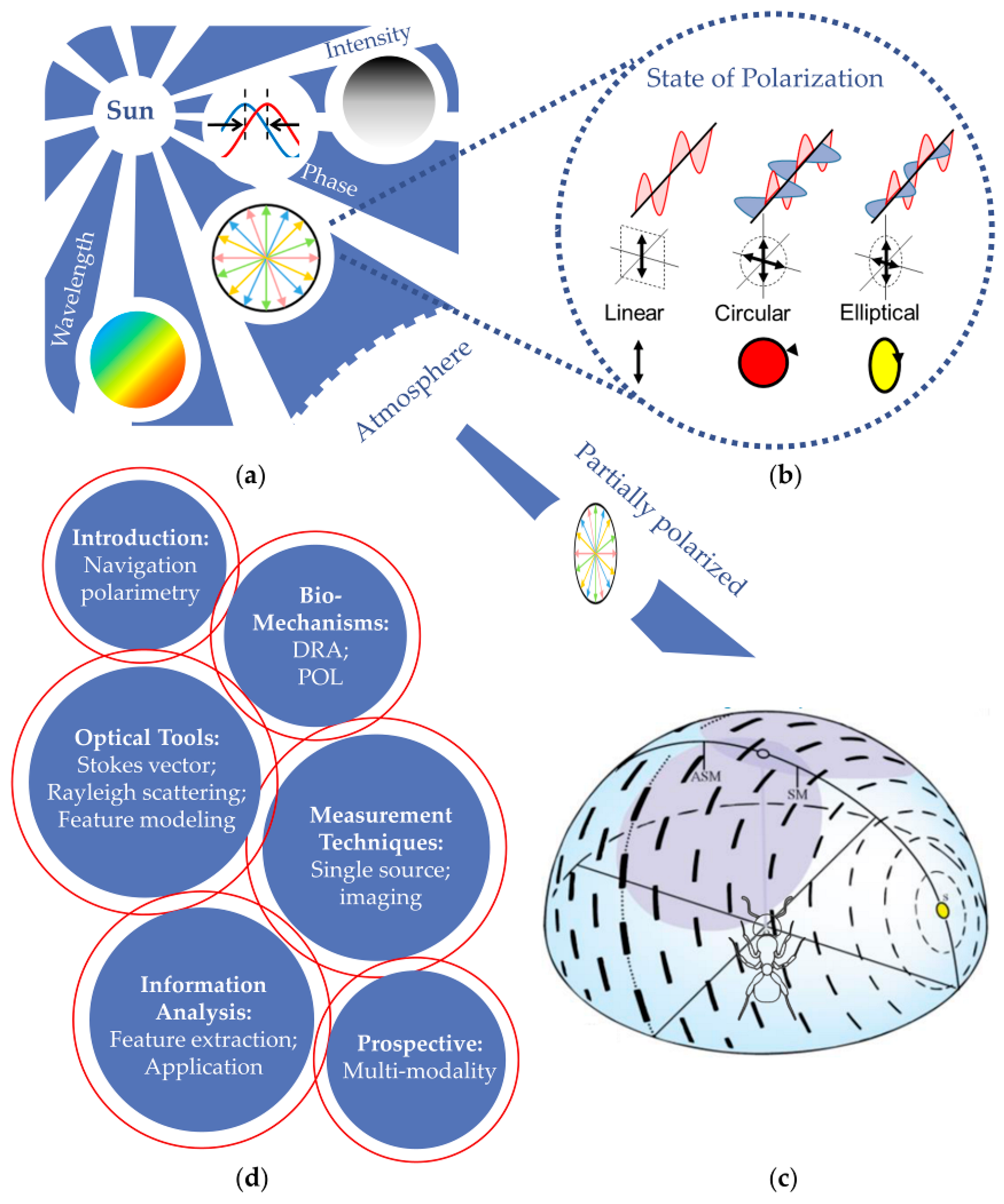
Light, as an electromagnetic wave, is characterized by the basic properties that are shown in Figure 1a, including intensity, wavelength, phase, and polarization [1,2]. While the former three are scalar, the polarization, which refers to the asymmetry of the direction of a light vector vibration relative to the direction of propagation (illustrated in Figure 1b), is vectorial. The exploitation of vectorial information requires more advanced optical and computational approaches. Hence, the study of polarization has passed through a shorter history compared with its scalar counterparts, and the extent of its applications is still being explored [3]. Polarimetry techniques seek to measure the polarization information of the optical field and further deduce the property of an object according to the light wave transmitted, reflected, refracted, scattered, and even diffracted by the object. So far, numerous areas have been reinforced with polarimetry techniques, ranging from basic research [3,4,5] to material and biomedical characterization [6,7,8] to remote sensing and geolocation applications [9,10,11,12,13].
Bionic geolocation and navigation is a novel application field facilitated by polarimetry techniques. It is inspired by biological discoveries of diverse animals completing foraging, homing, and long-distance migration by sensing the polarized skylight in the nature [14,15,16,17]. The physical basis of the behaviors of animals is the generation of the polarized skylight. After unpolarized sunlight enters the atmosphere, the atmospheric scattering process alters the vectorial property of the incident beam, resulting in changes in the degree of polarization (DoP) and the state of polarization (SoP) of the skylight observed on the earth [18]. Although affected by other transmission processes, including (but not limited to) refraction and absorption, these changes basically occur in a regular way, which makes the vectorial properties of skylight manifest a typical pattern across the whole celestial dome––that is, the skylight polarization pattern illustrated in Figure 1c [18,19]. The skylight polarization pattern is mainly determined by the relative position between the sun and the observation site on the earth, and it changes regularly under the common influences of time, orientation and environments [20,21]. Thus, it contains abundant pieces of directional and spatial information, and it provides a possibility for geolocation and navigation applications. Animals sense the skylight polarization pattern using a polarization-sensitive structure in compound eyes, and they figure out directions relying on the analysis of the polarization-sensitive nerve system [22,23,24], which enlightens human beings. The polarization of ubiquitous skylights has long been neglected because of the incapability of naked human eyes to perceive polarization directly. However, with advanced optical and computational approaches in polarimetry techniques recently, bionic geolocation and navigation that artificially senses the skylight polarization pattern and further deduces the directional information becomes possible [25]. Moreover, because of the anti-interference and the anti-cumulative error nature of the skylight polarization pattern, the bionic geolocation and navigation complements classic navigation methods and presents a promising prospect.
However, geolocation through artificially sensing polarized skylight faces the challenge of uncertainty in expected photon properties, which is introduced by the complexity of atmospheric transmission [26]. The turbidity of the atmosphere, weather conditions, and local environments impose randomness on the photons’ interaction processes [27,28]. These complicate the characterization, measurement, and analysis of vectorial information of skylight, and they distinguish the polarimetry for bionic geolocation applications from polarimetry techniques in other areas. In addition, polarimetry techniques in the field of material [29,30,31,32], biomedical [7,33,34], and remote sensing [35,36,37,38] etc. have been summarized in recent reviews. However, as a novel multidisciplinary field, there are few in-depth reviews of the progress in bionic geolocation and navigation. Hence, we hope to provide a comprehensive review of polarimetry for bionic geolocation and navigation with a specific focus on the appropriate characterization formalism, how to accurately and quickly measure the vectorial information of the skylight, and, finally, how to analyze available geolocation information from it.
The structure of this review is seen in Figure 1d. It consists of introducing the primary inspiration from the biological mechanism in Section 2, providing the basic polarization optical characterization tools in Section 3, summarizing the current measurement and analysis techniques of vectorial information in Section 4 and Section 5, respectively, and, finally, pointing out the possibilities for future multi-modal synergy with other cutting-edge technologies in Section 6. Bionic polarized skylight geolocation is now developing towards various directions in research and application fields, and we hope that this review could stimulate new explorations or breakthroughs in such prospective fields.
2. Biological Inspirations for Polarization Geolocation
The focus on the vectorial information of skylight for geolocation and navigation applications originated from biological research. As early as 1914, Felix Santschi found that after the sun was blocked, a variety of ants, including Cataglyphis, Monomorium, Messor, and Camponotus, were still able to return to their nests along a near-straight path after foraging [39]. It suggested that the sun is not their only source of geolocation information. In the 1940s, Karl von Frisch observed the same phenomenon in experiments on bees and revealed that polarized skylight is the true source of geolocation information with the physicist Hans Benndorf [40]. Since then, many scholars have conducted experiments to explore the polarized visions of various animals, such as Vowles’s and Carthy’s experiments on ants [14,41], Wellington’s experiment on flies [42], Papi’s experiment on beetles [43], and the experiments of Gomer et al. on spiders [40]. In addition, crickets [44], desert locusts [45,46], monarch butterflies [16,47], drosophila [17], and other organisms were also confirmed to navigate using naturally polarized skylight. More recently, the line of research has expanded from insects to migratory birds [48], some amphibians [49], reptiles [50], and bats [51] in mammals. Long-distance migratory birds may utilize the skylight polarization pattern during sunrise and sunset in order to calibrate their magnetic compasses [48]. The latest research proves that marine animals can also exploit polarization patterns in the sky as a compass for underwater geolocation [11,52,53].
There are two key issues in the animals’ geolocation based on skylight. One is how they detect the vectorial information from skylight, and the other is how they analyze vectorial information to achieve geolocation and navigation purpose. Solving the two issues is also the premise for human beings to realize polarization navigation through bionic approaches.
In order to answer the detection issue, a large number of experimental studies were carried out based on biological behavior, anatomy, electrophysiology and other methods, but it was not until 1970s that a breakthrough was made. As shown in Figure 2a,b, Schinz [22] and Wehner [23] successively found that the structure of ommatidia in the dorsal rim area (DRA) of insects’ compound eyes are quite different from others, and they proved that the DRA has the ability to detect polarized light. Taking the ommatidium in the DRA in Figure 2c [54], for instance, the retinula cells in the rhabdom extend a large number of microvilli from their membrane into the lumen of rhabdom. The arrangement of microvilli is chaotic in regular ommatidia, while the spatial arrangement of microvilli in DRA ommatidia is characterized by consistent axial rules and mutual vertical radial rules. The mutual vertical microvilli constitute a pair of detection channels for vectorial information, making the DRA very sensitive to the polarized light. By 1999, Labhart et al. [55] completed statistics on multiple insects, including odonata, orthoptera, coleoptera, lepidoptera, hymenoptera, and diptera, as shown in Figure 2d, and they indicated that the unique structure of DRA ommatidia is polyphyletic. Moreover, due to the wide range of comprehensive visual field of ommatidia in DRA, insects can capture a large range of skylight polarization information, reducing the influence of clouds, trees, and other interference factors, and then enhancing the robustness and absolute sensitivity of the polarized vision system. These superiorities are desirable in bionic polarization navigation, and the biological approaches provided inspirations for artificial measurements of polarized skylight. The ingenious DRA structure of the creatures offers a principle prototype for polarization measurement devices. The microvilli in ommatidia has the same effect as the polarization-sensitive components in artificial devices. The output of these inspirations will become apparent in Section 4.
The analysis of vector information mainly relies on polarization-opponent neurons (POL–neurons) in the optic lobe of the central nervous layer. In 1988, Labhart [56] discovered that when crickets were stimulated by polarized light with a continually rotating e-vector, the POL–neurons in their optic lobe exhibit spike activities between excitation and inhibition as well as the spike frequency was a sinusoidal function of e-vector orientation. This discovery first demonstrated the polarization opponent units of polarization sensitive nervous systems. After that, he found the same phenomenon in electrophysiological experiments on desert ants (Cataglyphis) [57]. In 2001, Labhart et al. [24] conducted statistical experiments on POL–neurons of crickets and divided POL–neurons into three types that were approximately tuned to e-vector orientations of 10°, 60°, and 130°, as shown in Figure 2e. The experimental results initially revealed the processing mechanism of polarization information in the optic lobe. The cricket conducts spatial integration to the response of three types of POL–neurons and obtain the angle between its body axis and the solar meridian to navigate. Taking advantage of the synergistic effect between the orthogonal polarization sensitive structure of ommatidia in DRA and the polarization analysis mechanism of POL–neurons in the optic lobe of the central nervous layer, the polarized vision system hardly depends on the intensity of the skylight. Indeed, the biological polarization geolocation can work regardless of various weather and illumination conditions, even under the moonlight [58,59]. Similar to the artificial measurement, creatures’ approaches inspired artificial information analysis for bionic geolocation applications, which is introduced in Section 5. In detail, more features for artificial polarization orientation, including (but not limited to) the solar meridian, are elaborated. Efforts to artificially adapt to the weather and illumination conditions are also reviewed.
Relying on the detection of polarized skylight based on DRA and the analysis of vector information based on POL–neurons, animals possess the ability of geolocation and navigation for foraging, homing, and long-distance migration. The path integration is regarded as desert ants’ main strategy of navigation with the skylight polarization information [60,61]. They extract directional information from the skylight polarization pattern, and they obtain mileage information through their proprioceptors. Using the dead reckoning, they always keep a vector pointing to the nest in their nervous system, and when they return to the vicinity of the nest, they will find the specific location by means of “snapshot”. Wittlinger et al. [62] demonstrated the pedometer capacity of proprioceptor by behavioral experiments that changes the leg length of desert ants. Wohlgemuth et al. [63] indicated that on account of the gravity proprioceptor, insects can also complete path integration in three-dimensional space. In 2008, Sakura et al. [64] proposed a programmable polarization information neural transmission model based on experiments of crickets’ POL–neurons, which simulated the whole process of organisms using the skylight polarization pattern to obtain orientation. In 2014, Jundi et al. [65] found that desert locusts and monarch butterflies integrate the skylight polarization information received by DRA and the spectral gradient information received by ommatidia in other areas of the compound eye to make course judgment during navigation.
Inspired by the above biological research, the bionic polarization navigation seeking to solve the measurement and analysis issues with artificial approaches is developed. However, since it is difficult for either human eyes or artificial detectors to directly measure vectorial information, appropriate characterization tools are needed before measurement and analysis.
3. Vectorial Characterization and Modeling for Bionic Geolocation Applications
The atmospheric transmission alters the polarization properties of the skylight, and creatures navigate according to the skylight polarization pattern. Hence, the premise of understanding and imitating biological navigational behavior is precisely characterizing the natural polarization properties of the skylight and establishing the light field model of the skylight polarization pattern. In this section, we first introduce the characterization tool of Stokes–Mueller formalism suiting bionic geolocation and navigation applications. On this basis, the modeling methods of the polarized atmospheric light field is subsequently reviewed.
3.1. Stokes–Mueller Formalism
Since light wave is a shear wave, the vectorial information of light is defined as the vibration of the electric field vector (e-vector). Jones formalism is a mathematical method of describing e-vector vibration in terms of amplitudes and phases, which is widely used in classic polarimetry, such as ellipsometry [66,67]. It consists of a two-element Jones vector describing the polarization of light and a 2 × 2 Jones matrix describing the polarization modulation of an object [68,69]. Jones vector represents the components of the e-vector in the x and y directions with two elements, and it can be visualized as a polarization ellipse. The Jones matrix is mostly used for transparent and non-depolarizing objects, such as thin films. However, atmospheric aerosol, clouds, and surface reflectance can arouse uncertainty in the vectorial properties of skylight, generating the depolarization effect, and this is difficult to characterize through Jones formalism [70,71]. This is because Jones formalism is intrinsically based on the assumption that the e-vector holds a particular ordered state, so it can only describe the fully polarized light. The vibration of partially polarized light (or fully depolarized light) is semi-disordered (or completely disordered), so more degrees of freedom are required in order to represent the light field. Considering that the skylight is dominated by partial polarization [18], and considering that the depolarization effect caused by atmospheric aerosol and cloud cover [70,71], another characterization, the Stokes–Mueller formalism, is generally used in bionic polarization navigation and geolocation.
The Stokes–Mueller formalism consists of a 4 × 1 Stokes vector characterizing the light and a 4 × 4 Mueller matrix describing the modulation of the object [72,73]. This formalism is widely used in polarized remote sensing and biomedical tissue polarimetry [7,9,38,74]. Neither the Stokes vector nor the Mueller matrix contains the absolute phase information, but they are devised with the same dimension as the light intensity, which is easy to measure. Thus, the Stokes–Mueller formalism can adequately describe fully polarized, partially polarized, and fully depolarized light, which is crucial in geolocation applications [75]. The experimental measurement process is also, in fact, a time-averaging process. Such averaging properties can also be found in the definition of the Stokes vector [76]. On the contrary, the Jones formalism is directly related to the expression of the analytical signal of the electric field vector, and it is therefore not suitable for either the expression of partially polarized light or the calculation of time average. It is more convenient to introduce the Stokes–Mueller formalism directly related to light intensity to measurement.
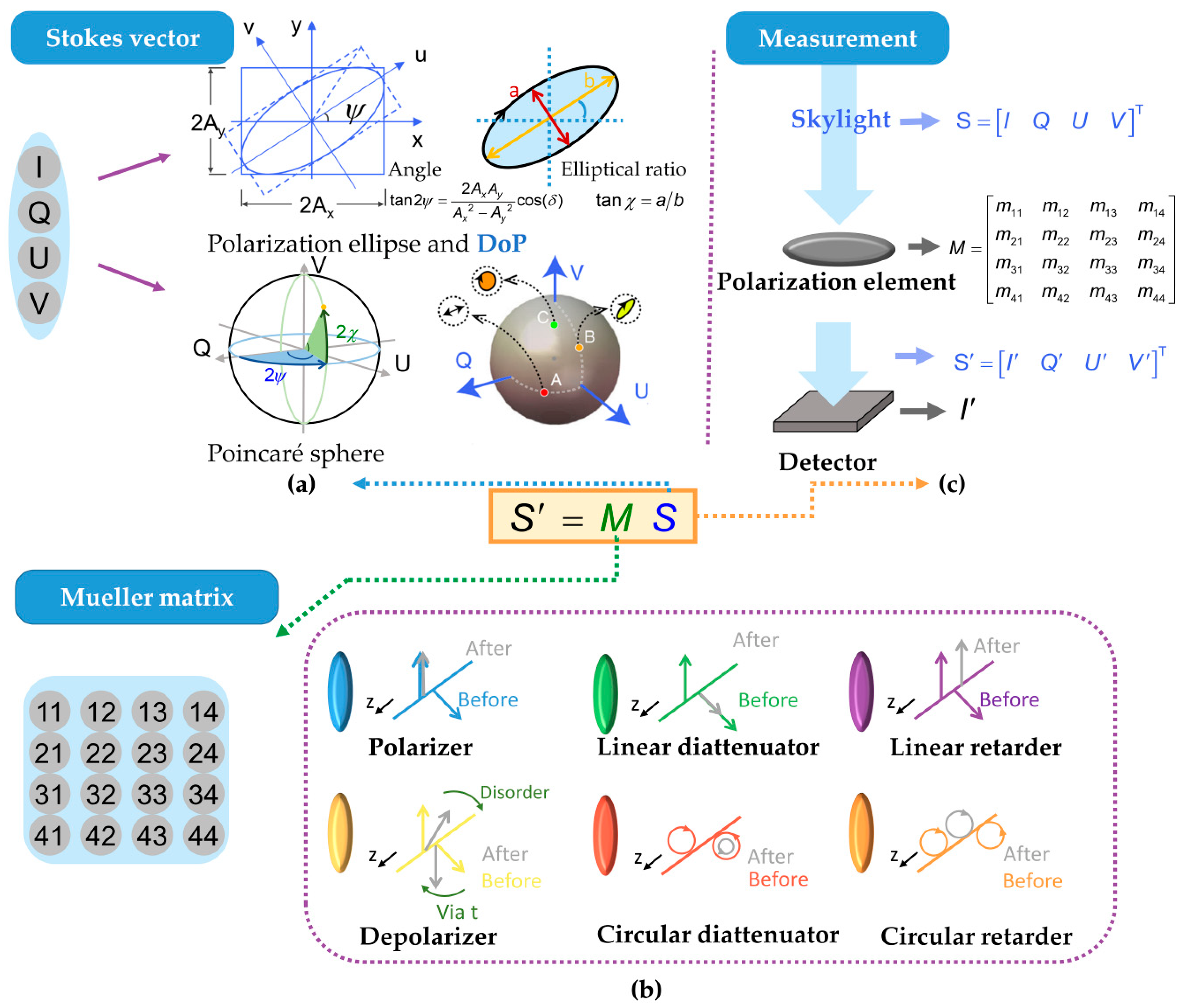
In detail, the Stokes vector consists of the set of parameters shown in Figure 3a, and the matrix form is expressed as follows [77,78]:
Practically, the Stokes vector is usually measured as:
where I is the total intensity of the light, Q is the difference between horizontal and vertical polarization, U is the difference between linear +45° and −45° polarization, and V is the difference between right and left circular polarization. These elements are often normalized to the value of I so that they have values between −1 and +1. Ex and Ey are, respectively, the components of the e-vector along the x- and y-axis in the vibration plane, and the vibrations along the x- and y-axis can be expressed with Ex = Axeiδ1 and Ey = Ayeiδ2. Re and Im, respectively, represent the real and imaginary parts of complex numbers. Graphically shown in Figure 3a, the Stokes vector can be represented by the combination of polarization ellipse and DoP. In the polarization ellipse, the two fundamental parameters, angle ψ, and elliptical ratio χ can fully represent the random shape and orientation of the ellipse, which suggests that the Stokes vector can describe all the SoPs. The Stokes vector is also visualized as a Poincaré sphere [79], suggesting both the SoP and the DoP. It represents partially polarized light as a point in the sphere and fully polarized light as a point on the sphere with linear states on the equator, circular states on the North and South Poles, and elliptical states in between.
On the basis of the Stokes vector, the polarization property of light in any SoP can be characterized, and some other parameters can be defined. The light observed in the nature is generally partially polarized, consisting of unpolarized component and polarized component. The proportion of polarized component is defined as degree of polarization (DoP) as:
The direction of the vibration of the e-vector is characterized by the angle of polarization (AoP) as:
Since there is almost no circular polarization component in skylight [19], and animals mainly sense the linear polarized information from the skylight for geolocation and navigation [74], the following discussion in this review is based on the neglect of circular polarized light in the skylight. The degree of polarization is simplified as degree of linear polarization (DoLP):
Because the intensity is the most intuitionistic property of light with the most mature measurement method, the Stokes vector is a convenient characterization for observation and measurement.
The Mueller matrix is a transmission matrix that describes the vectorial modulation properties of an object [77]. As illustrated in Figure 3b, the Mueller matrix expresses the full vector properties of an object through 4 × 4 elements (). Herein, represents the modulation (absorption or other loss) of the scalar intensity of light. The other 15 elements encode the vectorial modulation properties of the object, and the direct physical meanings of these 15 elements are normally ambiguous. Several basic modulations are encoded in the Mueller matrix as shown in Figure 3b, such as linear/circular diattenuation, linear/circular retardance, polarization, and depolarization [72]. Polarization properties of light before and after modulation of the element are graphically represented. These polarization elements are widely used in the measurement of the Stokes vector.
Based on the above vectorial characterization, the Stokes vector of skylight S is usually measured using the combination of a light intensity detector and a polarization element, as shown in Figure 3c. The skylight is modulated by a polarization element and then recorded by a light intensity detector. If and denote the Stokes vector of the incident skylight and the light received by the light intensity detector, respectively, is the Mueller matrix of the polarization element, and the process can be expressed as . Taking a polarizer as the polarization element, the measurement process is expressed as:
The φ is the angle between the x-axis direction of the measured light and the polarization direction of the polarizer. After modulation, I′ in S′ is measured to construct an equation with S and the first row of M.
Owing to the ignorance of the circular polarized light, the fourth component V defaults to 0 [80], and only the first three components of S remain to be measured. However, the light intensity detector can only detect the total intensity I′. Obviously, one equation is not enough to solve the three unknowns, I, Q, and U, and more constraints are needed. The constraints can be obtained by extending the temporal dimension, e.g., conducting multiple measurements or the spatial dimension, e.g., increasing measurement channels and dividing the focal plane, which is interpreted in detail in Section 4.
The Stokes vector and the Mueller matrix can well represent the vectorial properties of the skylight itself and the modulation characteristics of the measurement, and they are suitable for characterizing the partial polarization and the depolarization caused by complex atmospheric transmission. Thus the Stokes–Mueller formalism has been the most mainstream representation method for vectorial information of the skylight adapted to geolocation and navigation applications [13,74].
3.2. Atmospheric Polarized Light Field Modeling
With the appropriate characterization tool, the Stokes-Mueller formalism, the methods to model the skylight polarization pattern can be generally divided into two categories. The first one is modeling the skylight polarization pattern by solving the vector radiative transport equation (VRTE) of light [81,82,83,84]. The complex changes of the light field in the whole atmospheric transmission are derived from the set parameters and conditions mainly using the matrix operator [84], discrete ordinate theory [85], spherical harmonics expansion [86], and multiple scattering theory [87]. The calculated result of the skylight polarization pattern is very accurate, but this method only can be applied on the premise that the precise composition of the target atmosphere is known. Because of the high computational complexity, modeling methods based on the VRTE require a large amount of time. For geolocation and navigation applications, the precise composition of the target atmosphere is usually unknown, and there is a high requirement for real-time performance. This method is more suitable for the theoretical study of the skylight polarization pattern than the applied research. The other method is establishing an analytical model of the skylight polarization pattern from the perspective of feature description. Because the bionic geolocation and navigation is not concerned with elaborate changes of polarized light in the transmission process, but with the overall pattern and features of the polarized skylight, this kind of method is more prevalent in the experimental and applied research in this field.
Among the existing analytical models of the skylight polarization pattern, the Rayleigh single scattering model [88,89] is the most classical model. This model is based on the assumption that the ratio (x) between wavelength (λ) and radius (r) of atmospheric particles, x = 2πr/λ, remains far less than 1, and the scattering process can be described by the Rayleigh scattering theory. As shown in Figure 4a, the oscillating electric field of the incident light acts on the charges within a particle, causing them to move at the same frequency and thus making the particle become a small radiating dipole [88]. The size of atmospheric molecules falls to the range of ratio. According to Rayleigh scattering theory, if the incident light with wavelength λ and intensity I0 is scattered by an atmospheric molecule, the intensity of the scattered light is given by:
where R is the distance to the molecule, γ is the scattering angle, and α is the molecular polarizability proportional to the dipole moment induced by the electric field of the light. The changes of components of the electric field vector in the x and y directions can be expressed as:
where Ex and Ey represent the components of the electric field vector of the scattered light in the vibration plane, and E0x and E0y represent the components of the electric field vector of the incident light. means positive correlation.
Hence, the atmosphere observed at the observing position on the earth (O point) is modeled as a hemisphere, as shown in Figure 4b. Z represents the zenith. The S and P on the hemisphere, respectively, represent the position of the sun and the scattering particle. The e-vector of the scattered light beam received by observer, illustrated by in Figure 4b, is always perpendicular to the scattering plane determined by OPS. The AoP and the DoLP distribution according to Rayleigh single scattering theory is derived from Equations (7) and (8) and shown in Figure 4c,d.
As shown in Figure 4c,d, the Rayleigh single scattering model concisely represents some basic features of the real skylight polarization pattern, such as the position of the sun, the solar meridian and antisolar meridian (SM–ASM), and the ∞-shape feature shown by the pale purple dotted line in Figure 4c. The position of the sun is the most decisive feature of the skylight polarization pattern. It is generally expressed by the azimuth angle () and the zenith angle () of the sun in the observation coordinate system. The SM–ASM is the straight line crossing through the zenith and the sun, about which the skylight polarization pattern is symmetric. If two AoP contours line negative to each other is drawn, they manifest a ∞-like shape with the SM–ASM as an axis in the distribution of AoP. These features can be extracted and analyzed for geolocation and navigation, which is detailed in Section 5.1.
However, owing to the neglect of some factors, differences still exist between the skylight polarization pattern simulated according to the Raleigh single scattering theory and the real one sensed by biological compound eyes. Firstly, Rayleigh scattering does not take the wavelength and the intensity of the skylight into account, while intensity is nonuniform across the celestial dome [90], and most of the biological compound eyes on DRA only respond to monochromatic light [91]. To compensate for the differences in the wavelength and the intensity, Wilkie et al. [92] proposed an analytical model for skylight polarization concerning the intensity; Nishita et al. [93] and Wang et al. [94] introduced a wavelength control factor to the skylight model. Secondly, the depolarization in the skylight polarization pattern is not taken into account in the Rayleigh single scattering model. The maximum value of DoLP identically equals 1 in the Rayleigh single scattering model, but the actual DoLP in the celestial dome scarcely reaches 1 because of the multiple scattering effects [92]. Moreover, the existence of four neutral points where the emitted light is unpolarized (DoLP equals 0) has been verified and studied widely [70,95,96,97], but it cannot be correctly described under the framework of the Rayleigh scattering theory. To model depolarization phenomena, Berry et al. [98] proposed a singular value model to describe the existence of neutral points, and Hannay [99] presented a model to characterize the multiple scattering. With the above efforts, although analytical models are originally established from the perspective of feature description, they are refined and very close to the real skylight polarization pattern.
It should be noted that there are some large-scale particles in the atmosphere, including cloud droplets, aerosols, ice crystals, dust, and so on, and that the Rayleigh theory cannot describe their scattering process. When the ratio x = 2πr/λ is comparable to or slightly larger than 1, scattering events are described with Lorenz–Mie scattering theory [100], which is shown in Figure 4a. The even larger x (x > 50) falls into the category of geometric optics. Because the atmosphere mainly consists of molecules, the Rayleigh single scattering is absolutely predominant in clear sky. Only in cloudy, foggy and rainy weathers, the effect of Lorenz–Mie scattering emerges obviously [101]. Under these conditions, the skylight polarization pattern considerably differs from Rayleigh single scattering model, and the specific analysis methods are required and elaborated in Section 5.2.1. To sum up, this section provides theoretical tools including characterization and models for the practical measurement and the analysis of vectorial information in Section 4 and Section 5.
4. Vectorial Information Measurement for Bionic Geolocation Applications
Similar to the function of DRA in biological compound eyes, the realization of bionic polarization geolocation first relies on the measurement of skylight vectorial information. As shown in Figure 5, this section divides measurement methods into two categories according to the range of sampling: point-source measurement and imaging measurement method.
4.1. Point-Source Measurement
The method of point-source measurement can measure the polarization properties of a point or several points in the celestial dome. The sensor used for this method is mainly photodiode, which is generally in conjunction with some polarization elements (such as polarizers, retarders, etc.) and signal processing devices (such as operational amplifiers).
In 1981, Brines et al. [20] designed a set of point-source measurement device and utilized this device to measure the skylight polarization pattern by scanning at every 5° solar elevation and azimuth. By 1997, Lambrinos et al. [25] were inspired by the biological DRA structure and POL–neurons, and thus they established the original prototype for geolocation according to polarized skylight. They mounted a photodiode, a linear polarizer, and a blue transmission filter in a cylindrical brass tube to simulate the polarization-sensitive receptor of DRA in compound eye, and they measured the polarized skylight with six such tubes. They equipped the mobile robot Sahabot with this point-source measurement device, and they completed autonomous navigation experiments according to the path integral principle [102]. Subsequently, researchers such as Labhart [103], Chu [104,110], and Sarkar [111] improved the point-source measurement device and made it more integrated. Higashi [112] and Chahl [113,114] conducted navigation experiments based on the point-source measurement method with a wheel robot and unmanned an aerial vehicle separately.
The device of point-source measurement is simple in structure and very low in cost. However, the disadvantages of point-source measurement are also very obvious. Photodiode can only measure the polarization property at a certain point or several points in the sky scene, resulting in an extremely limited field of view susceptible to interference from climate conditions and measurement environments. Moreover, it takes a long time and a huge workload to acquire the whole skylight polarization pattern with point-source devices. The long-term measurement process and frequent adjustments undoubtedly introduce more error sources.
4.2. Imaging Measurement
Compared to the point-source measurement, which is highly susceptible to interference, the imaging measurement method captures polarization images with a large field of view and has higher stability and robustness. Research on polarization imaging measurement has been going on since the 1970s, but the photographic film was needed to record images in early days [115]. At present, the imaging measurement of polarized skylight mainly relies on image sensors, which is generally in conjunction with optical objective, polarization elements (such as polarizers and retarders), and other optical components (such as beam splitters). The method of imaging measurement can measure the vectorial information of the skylight within a part of or even the entire hemispherical sky region and establish a two-dimensional description of the polarization pattern in the region, which is usually expressed and recognized in the form of images [37].
Akin to many other measurement methods, the imaging measurement of the vectorial information of the skylight is also a study in compromises between time and space. As mentioned in Section 3, this is essential because the Stokes–Mueller formalism is multi-dimensional and can only be derived using multi-frame images. Ideally, if the measurement is extended from the time dimension, at least three shoots are required owing to the existence of circularly polarized light that can be neglected in bionic geolocation applications. Since the polarization pattern is obtained by manipulating the same pixel across multiple sequential frames, any motion in the image scene during the three shoots, whether generated by the scene itself or by the motion of the measuring platform, leads to artifacts, which may obscure the true polarization pattern [37]. The best solution to minimize these artifacts is to acquire multiple images simultaneously, that is, to extend the measurement from the spatial dimension. Conceptually, the easiest way to extend the spatial dimension to measure polarization information is to use multiple discrete cameras with separate optical systems and align them to capture the same part of the scene [37]. However, a point in the scene is actually projected into multiple images with slight field-of-view deviations. The difficulty turns out to be the complex spatial registration between images that needs to correct both mechanical misalignment and aberrations caused by the separate optical paths.
This subsection details three types of the most commonly used imaging polarimetry devices for geolocation applications: the division-of-time polarimeter, the division-of-channel polarimeter, and the division-of-focal-plane (DoFP) polarimeter. Among them, the first one obtains the necessary multidimensional information in terms of time, and the others choose to extend the measurement from the spatial dimension. In addition, a significant limitation of imaging measurement device is that the optical axis constantly points to the zenith, which brings extra difficulties for airborne platforms [114]. To overcome the limitation, Stürzl et al. [116] proposed a set of solutions to deal with the roll and the pitch of the platform and realized imaging polarization measurement on an unmanned aerial vehicle.
4.2.1. Division-of-Time Polarimeters
Division-of-time polarimeter is a common polarization measurement method for geolocation and navigation applications. It alters modulations on polarization property by changing the polarization elements multiple times during a single measurement, and thus satisfies the required dimensions for the calculation of Stokes vector in terms of time [117,118]. For the measurement of skylight that only concerns linear polarization, the polarization elements are usually linear polarizers and retarders [119].
The division-of-time polarimeter was applied to the vectorial information of skylight by Voss et al. [120,121]. They designed a polarization radiance distribution camera system (RADS-IIP) based on a fisheye lens, a CCD camera system, and a dichroic sheet-type polarizer built into the camera system. According to the principle mentioned in Section 3.1, the linear polarization components of the incident light field can be determined by changing the polarizer and capturing sequential images. The accuracy of RADS-IIP was verified to be comparable to that of the point-source polarimeter. Qualitatively, the dependence of polarization characteristics on wavelength, solar zenith, and surface albedo measured with RADS was accordant with the Rayleigh scattering model presented in Section 3.2.
This division-of-time polarimeter is attractive because its system design is relatively simple, and easy to build [105,106,107,122,123,124,125]. However, the obvious drawback is that both the scene and the measurement platform must be stationary during measurement to avoid introducing the inter-frame motion. In early studies, the polarizers were often mounted directly in front of the camera and rotated manually, which was too slow to achieve a reasonable frame rate. In daylight, each time of measurement using RADS-IIP took 1.5–2 min [120]. In order to improve measurement speed, Gal [105,126,127] and Pomozi [128,129] improved the division-of-time polarimeter with a built-in wheel that was equipped with three polarizers in different directions. Under lighting conditions of sunny and clear daylight, a complete measurement with the polarimeter still requires 6–8 s, and it uses photographic latex detectors, which have a more limited dynamic range than CCD detectors. Driving the polarization element with a motor instead of manual labor can effectively shorten the time interval between two frames of images [123,130,131,132]. Despite the recent success in shortening measurement time and improving frame rate, if there is sufficient movement in the scene or measurement platform during the acquisition process, such as a bird or a plane flying over the sky, the fast-changing solar radiation during sunrise and sunset, and a fast-moving carrier of measurement platform, beam drift can still cause artifacts.
In addition, the rotation of elements may also introduce unexpected errors because of the mechanical motion [133]. For circumvention, researchers attempted to reduce the number of rotating elements or replace traditional polarization elements of the polarimeter with fast modulation elements, such as liquid-crystal variable retarder (LCVR) [134,135,136], spatial light modulator [137], and the ferroelectric liquid-crystal modulator [138,139]. For instance, the LCVR can provide tunable retardation by changing the effective birefringence of the material with the applied voltage, thus modulating the SoP of skylight rapidly without mechanical motion [140]. The dual field-of-view imaging polarimeter based on LCVR takes only 0.4 s to obtain the full-polarization images [134]. With proper improvements, the division-of-time polarimeter can provide favorable results with a relatively small investment in hardware, design, and integration.
4.2.2. Division-of-Channel Polarimeters
The architecture of the division-of-channel polarimeter is based on multiple separate camera systems, which are coaxial calibrated and equipped with different polarization elements. Thus images with different modulations can be obtained from multiple channels at the same time. It is the simplest and the most direct way to obtain the required dimensions in terms of space.
In 1981, North et al. [141] designed a division-of-channel polarimeter based on a four-lens stereoscopic camera, four linear sheet polarizers, and a dome mirror, and they applied the polarimeter to atmospheric polarization pattern measurement. However, the large and bulky dome mirror can hardly capture the whole sky scene. Since only the first three parameters of the Stokes vector make sense for skylight, Horvath et al. [109] simplified the above structure and developed a three-lens three-camera full-sky imaging polarimeter. They lined up three cameras and used fisheye lenses with built-in 0°, 60°, and 120° polarizers to modulate the polarization property and acquire the polarization pattern of the whole sky scene. Wang et al. [142] extended the point-source polarimeter and presented an imaging polarimeter with three channels. By installing and uninstalling lenses in front of the camera system, both point-source and imaging measurement can be completed.
Polarization imaging measurement with this multi-channel structure has been widely used in geolocation and navigation applications [108,143,144]. However, the spatial registration between images of different channels is very complicated because there exist both optical aberrations caused by discrete optical paths and mechanical misalignments caused by installation [37]. Although the calibration of a single camera has been studied extensively [145,146], there is no universal calibration algorithms for division-of-channel skylight polarimeter. Some self-calibration techniques for the multi-camera system can be utilized [147,148,149]. For the division-of-channel skylight polarimeter, Fan et al. [150] and Wang et al. [151] proposed specific calibration algorithms and applied them in the measurement of the polarized skylight. Owing to the complicated spatial registration problems, the discrete division-of-channel polarimeter is hard to execute precisely. On this foundation, various integrated imaging polarimeters, such as the DoFP polarimeter, have turned out to be widely utilized in recent years.
4.2.3. Division-of-Focal-Plane Polarimeters
Until recently, with the maturity of micro and nanofabrication, micro-optical polarization elements were directly integrated into the focal plane array (FPA) to modulate the polarization properties in the pixel-scale, forming the new division-of-focal-plane (DoFP) polarimeter [152]. Although some other integrated polarimeters, such as the division of amplitude polarimeter [96,153,154,155,156] and the division of aperture polarimeter [157,158], have been utilized in the measurement of skylight polarization information, the DoFP polarimeter has gradually developed into a prevailing technology in the field of polarization skylight measurement due to its small size, good compatibility, simultaneous imaging, and applicability to dynamic scenes.
In 2009, Sarkar et al. [111,159] designed a DoFP-type bionic polarization sensor consisting of multiple groups of detection units manufactured on CMOS micro-structure. The cross-section of the sensor includes a 64 pixel × 128 pixel region to detect unpolarized information and two 64 pixel × 64 pixel regions to simultaneously acquire polarized light information. In 2010, Gruev [160] reported a polarization imaging detector that captures the optical properties of polarized light by singly integrating an aluminum nanowire filter with a pixel in the CCD imaging array. The detector consists of 1000 × 1000 pixels with a pixel spacing of 7.4 µm, covered with an array of nanowire polarizer filters with four different orientations offset by 45°. The detector has a signal-to-noise (SNR) ratio of 45 dB in the visible spectrum at 40 frames per second with 300 mW of power consumption. Garcia et al. [53] mimicked the vision system of mantis shrimp and developed a single-chip, low-power, high-resolution color-polarization imaging system by monolithically integrating nanowire polarization filters with vertically stacked photodetectors, as shown in Figure 5l. The following year, they developed a 384 × 288 pixel polarization imaging sensor with a high dynamic range utilizing 250 nm high × 75 nm wide aluminum nanowires, achieving a dynamic range of 140 dB and a maximum SNR of 61 dB at 30 frames per second [161]. In 2018, Sony Corporation launched an IMX250 MZR polarization image sensor, whose structure can minimize the crosstalk of polarized light in different directions as shown in Figure 5k. Companies such as FLIR and Lucid Vision Labs have followed suit with monochrome and color DoFP polarization cameras. Because of their compact, stable, and real-time characteristics, the commercial products of polarization cameras have become more and more preferred in the studies of polarization skylight measurement nowadays [96,162,163], and they promote further development in bionic polarization geolocation and navigation.
The significant advantage of the DoFP polarimeter is that it makes a better compromise between the consideration of time and space. With the nanowire structure, the measurement can be completed synchronously for each pixel and multiple polarization images with different modulations can be obtained simultaneously by splitting and rearranging the pixels. Compared with a division-of-channel polarimeter, discrete optical paths, bulky volume, and mechanical misalignments are no longer in existence, and optical aberrations are largely cut down. However, the DoFP polarimeter must trade off the spatial resolution of the polarization information. Because of the micro-optical polarization element integrated on the sensor, a pixel can only record one of the intensities of polarized light oriented towards 0°, 45°, 90°, and 135°, resulting in a loss of spatial resolution. To address this issue, most DoFP systems set interleaving superpixels. A typical DoFP system will estimate the Stokes vector of a pixel using several nearby pixels on the focal plane.
The main error source of the DoFP polarimeter is non-consistency errors and instantaneous field of view (IFoV) errors [164]. Among them, the non-consistency errors between pixels are caused by the manufacturing and assembly errors of the micro-polarizer array and the detector noise. For non-consistency errors, calibration is an effective way to remove them [164,165,166,167,168]. The IFoV errors occur because the instantaneous fields of view of adjacent pixels do not overlap. Through the setting of surperpixels composed of adjacent pixels, the IFoV can be reduced to a 1-pixel registration error. Many interpolation methods are also proposed to minimize the IFoV error while simultaneously minimizing the information loss due to the limited spatial resolution [169,170,171,172].
5. Vectorial Information Analysis for Bionic Geolocation Applications
Mimicking the function of the POL–neurons in the optic lobe of the central nervous layer, the measured vectorial information need to be artificially analyzed for geolocation and navigation purpose. This section introduces the universal features of polarized skylight and corresponding processing methods under normal sunny and clear daylight. Specific analysis methods adapted to multifarious climate and environmental conditions are then discussed.
5.1. Vectorial Feature Extraction
As introduced in Section 3.2, atmospheric scattering makes the polarization properties of skylight manifest a pattern on the celestial dome. Under sunny and clear days, the skylight polarization pattern is concisely represented by Rayleigh single scattering model, and some universal features are stable and regular. Thus, these features can be extracted to determine the skylight polarization pattern under sunny and clear daylight. The features of the skylight polarization pattern include the position of the sun, the solar meridian and antisolar meridian (SM–ASM), the ∞-shape feature, and the neutral points.
The position of the sun, which is extracted as the solar azimuth angle and the solar zenith angle (or altitude angle), is the most basic feature of the skylight polarization pattern. On the basis of solar azimuth and solar zenith, the latitude and longitude information can be retrodicted to complete the geolocation of the carrier [173]. To extract the position of the sun, Hamaoui [174] developed a gradient-based technique for recovering the sun’s azimuth and elevation angles from sky polarization images. Liu et al. [175,176] determined the position of the sun indirectly through extracting the ∞-shape feature from the image of AoP. They established a dataset of ∞-shape features properly according to Rayleigh scattering theory, and they derived the position of the sun by maximizing a similarity index between the extracted ∞-shape feature and the Rayleigh ∞-shape feature.
The SM–ASM is an important inherent important feature of the skylight polarization pattern. Ma et al. [177] proposed an algorithm to extract the SM–ASM according to the symmetry, and proposed an evaluation of AoP of skylight. Lu et al. [123] completed the extraction and the angle solving of SM–ASM through the Hough transform algorithm in the field of machine vision. The accuracy of the algorithm was tested better than 0.34° with a simulation experiment. When the algorithm was tested on a division-of-time polarimeter, the measurement accuracy was better than 0.37°. They [123] then simplified multiple nonlinear calculations in the analysis of vectorial information, which improved the efficiency of the algorithm. Tang et al. [143] proposed an SM–ASM extraction method based on a pulse-coupled neural network (PCNN) and a linear fitting algorithm. PCNN was used to filter the feature points of the solar meridian, and then the linear fitting method was used to calculate the angle of the SM–ASM. In 2018, Zhao et al. [136] set a symmetry index for the skylight polarization pattern, and extracted the exact SM–ASM direction based on symmetry axis scanning and curve fitting. Liang et al. [156] transformed the issue of extracting SM–ASM into a binary classification problem and used a soft-margin support vector machine to solve this issue. Guan et al. [178] proposed a method based on polar coordinate transformation to extract the SM–ASM with a single-pixel ring.
The neutral point where the skylight is depolarized is another significant feature of the skylight polarization pattern [98,99]. As introduced above, Rayleigh’s theory [19] well describes the dominant trend of optical polarization properties of the skylight. However, the actual skylight polarization pattern differs from the ideal Rayleigh model in detail. These differences, known as polarization defects, are caused by multiple scattering, molecular anisotropy, size and shape distribution of aerosol particles, and reflection from the ground [95]. The neutral points existing in the real skylight polarization pattern are the most obvious polarization defects, where DoP values equal to 0. At present, it has been found that there are four neutral points in the plane of SM–ASM, namely, Arago neutral point [179], Babinet neutral point [180], Brewster neutral point [181,182], and the fourth neutral point [70,95,105]. Usually, in the clear sky of daylight, only two neutral points above the horizon can be observed. The distribution of neutral points has obvious directional characteristics, which can be used as a reference to provide accurate direction information for autonomous navigation. The main methods to extract neutral points are based on DoP images, including the geometric centroid method [105,183,184], ellipse fitting method [185], and the method based on the intersection features of the neutral lines [185]. Recently, some extraction methods based on AoP images have also been proposed [96]. It is worth mentioning that because the positions of the neutral points are closely related to the atmospheric turbidity, the observation of the neutral points can also guide the monitoring of atmospheric environmental quality [96,186].
5.2. Vectorial Information Analysis Adapted to Specific Conditions
Under some specific atmospheric and weather conditions, the skylight polarization pattern largely differs from that in sunny and clear days. In addition, the environmental conditions of the observation site may also introduce some interferences. To extend the adaptability of the geolocation and navigation method based on the skylight polarization pattern, plenty of studies of the specific conditions have been conducted.
5.2.1. Atmospheric and Weather Conditions
The polarization characteristics of the skylight under complex atmospheric and weather conditions have been the focus of researchers for years. Konnen [187] indicated that under cloud and fog conditions, the polarization degree of the skylight would decrease overall due to the influence of multiple scattering. Nathan et al. [101,134] found that this kind of reduction is more significant in the longer-wavelength band. Ugolnikov et al. [188,189] studied the depolarization effect of multiple scattering and the stratosphere under twilight daylight. Hegedüs et al. [190] published testing research on the polarization pattern of thick clouds and found that although the DoP of skylight in foggy and cloudy weather is relatively low, the AoP is qualitatively the same as that of the clear sky. Miyazaki [191] subsequently measured the skylight polarization on clear and cloudy days with an imaging polarimeter and compared it with the skylight polarization pattern of the Rayleigh model, drawing similar conclusion to previous studies. On this basis, many specific algorithms of analyzing the skylight polarization have been proposed to adapt to multiple atmospheric and weather conditions [136,142,143,156,177].
Some researchers explored the possibility of night navigation based on the skylight polarization pattern [184,192,193]. The night light source is mainly composed of sunlight, moonlight, and other cosmic light, where the sunlight reflected by the moon accounts for the main part of the light source [127,194]. Jensen et al. [195] established a physical model of the night skylight and analyzed the main components of the skylight as well as the influence of different light sources on the night imaging effect. In addition, the atmospheric polarization patterns during eclipses were also studied [97,183,196]. The mechanism of the navigation of aquatic animals using polarized skylight was also being researched [11,52].
5.2.2. Environmental Conditions of the Observation Site
On the ground, the obstructions of buildings and trees bring challenges for bionic geolocation and navigation based on the polarized skylight [108,119]. Obstructions block the sky scene and make the detected skylight polarization pattern incomplete [197]. Thus some specific algorithms were proposed to solve the issue [143,144,163].
On the ocean, the scattering is even more complicated owing to the thick water clouds. Hegedüs [198] studied the skylight polarization patterns on cloudy and foggy days over the Arctic Ocean. Cui et al. [199] simulated and measured the marine polarization pattern over the Yellow Sea, and conducted a comparison with terrestrial polarization patterns. Liu et al. [200] established the atmospheric polarization model of water clouds, and analyzed the correlation between the optical band, aerosol, water cloud physical parameters, and the skylight polarization pattern. They proved that the DoP decreases with the increase in the optical thickness and the decrease in the effective radius of the water cloud, and the longer the wavelength, the more obvious the decreasing trend of the polarization degree. Experiments showed that the marine skylight polarization pattern is similar to that of the land under clear day, and the skylight polarization pattern is still considerable when the humidity is high [124]. The skylight polarization distribution pattern over the sea can still be applied in the field of polarization navigation [126]. On this basis, Zhou et al. [201] studied the polarization patterns of skylight when reflected off the surface of waves and provided a reference for optimally diminishing the reflected skylight. Barta et al. [202] detected cloud cover by measuring the polarized skylight under the extreme environmental conditions of a trans-Atlantic voyage.
6. Development Directions for Polarization Geolocation and Future Prospects
Bionic polarization geolocation and navigation technology has shown its superiority in many aspects. Although the most widely used global navigation satellite system (GNSS) has high precision, GNSS is incapable in some special cases where the satellite signal is interfered with or destructed [203], and some passive approaches are called for as a supplement. There are some defects in conventional aided alternatives. The geomagnetic navigation system is plagued by abnormal local electromagnetic environments because it works by sensing the real-time magnetic field and matching it with the pre-measured database [204]. The inertial navigation system functions independently based on accelerometer and gyroscope devices, but the error accumulates over time inevitably [205]. The bionic polarization geolocation and navigation technology can complement these defects. The skylight polarization pattern occupying the whole celestial dome is difficult to completely damage or interfere with, so it can provide a stable and continuous source of directional information. In addition, accumulative errors are inherently avoided because the pattern is an absolute and real-time reference.
Since the polarization geolocation and navigation is a multi-discipline-crossing edge field involving the biology, optics, robotics, computer science, and so on, it is advancing in multiple directions. We hope that this review gives the readers a general overview of fundamental mechanisms and concepts, measurement techniques, information analysis, and current applications. In addition to the summaries of existing research, we provide here some further perspectives on prospects in this area.
Firstly, biology discoveries on the polarization vision system are no doubt going to inspire new bionic breakthroughs [11,53,192]. At present, the ability of the polarization vision system to detecting and process has been imitated in devices and algorithms separately [12,13,55]. However, some exact mechanisms, for instance, by which animals’ polarization navigation works so robustly adapt to various climates, illuminations, and environments still remain mysterious. Multitudinous studies are ongoing, and more results are expected [206,207,208].
Secondly, a multimodal combination with other advanced technologies is going to improve the optical and computational approaches of the bionic polarization navigation. The fast development of machine learning is clearly going to have an impact on this field [209,210]. Such data-driven techniques may pave new directions for polarization navigation, either by improving the quality of polarimeter (such as overcoming the numerous sources of measurement error) or through enhanced information extraction (such as resisting to overcoming the numerous extreme conditions) [209,210,211]. One possibility is to utilize defective polarization images to predict the skylight polarization patterns [163]. Moreover, the cutting-edge techniques based on metasurfaces are clearly going to bring new opportunities for advanced polarimetry, such as forming compact vectorial sensors. The metasurface of subwavelength, anisotropic structures have been adopted for full-Stokes polarization imaging [212]. A high-sensitivity, ultra-thin polarization camera based on compound-eye metasurface optics is already proposed [213].
Finally, the polarization skylight measurement has been fused with multiple sensing methods to extend its application on geolocation and navigation [144,214,215]. Further fusion with other navigation methods related techniques may again open windows for the polarization navigation with multi-modal performance.
Author Contributions
Conceptualization, Q.L.; writing—original draft preparation, Q.L.; writing—review and editing, Q.L., L.D., Y.H., Q.H., W.W., J.C. and Y.C.; supervision, L.D., Y.H., Q.H., J.C. and Y.C. All authors have read and agreed to the published version of the manuscript.
Funding
This research was funded by Beijing Nature Science Foundation of China, grant number 4232014; SongShan Laboratory Foundation, grant number YYJC072022008.
Data Availability Statement
No new data were created for this article.
Conflicts of Interest
The authors declare no conflict of interest.
References
- Ronchi, V.; Barocas, V. The Nature of Light: An Historical Survey; Harvard University Press: Cambridge, MA, USA, 1970; ISBN 100674605268. [Google Scholar]
- Huard, S. Polarization of Light; Wiley-VCH: Hoboken, NJ, USA, 1997; ISBN 0471965367. [Google Scholar]
- Zhan, Q. Cylindrical Vector Beams: From Mathematical Concepts to Applications. Adv. Opt. Photonics 2009, 1, 1–57. [Google Scholar]
- Ndagano, B.; Perez-Garcia, B.; Roux, F.S.; McLaren, M.; Rosales-Guzman, C.; Zhang, Y.; Mouane, O.; Hernandez-Aranda, R.I.; Konrad, T.; Forbes, A. Characterizing Quantum Channels with Non-Separable States of Classical Light. Nat. Phys. 2017, 13, 397–402. [Google Scholar]
- Wang, J.; Castellucci, F.; Franke-Arnold, S. Vectorial Light–Matter Interaction: Exploring Spatially Structured Complex Light Fields. AVS Quantum Sci. 2020, 2, 031702. [Google Scholar] [CrossRef]
- Schulz, M.; Zablocki, J.; Abdullaeva, O.S.; Brück, S.; Balzer, F.; Lützen, A.; Arteaga, O.; Schiek, M. Giant Intrinsic Circular Dichroism of Prolinol-Derived Squaraine Thin Films. Nat. Commun. 2018, 9, 2413. [Google Scholar]
- Ghosh, N.; Vitkin, A.I. Tissue Polarimetry: Concepts, Challenges, Applications, and Outlook. J. Biomed. Opt. 2011, 16, 110801. [Google Scholar]
- He, C.; He, H.; Chang, J.; Chen, B.; Ma, H.; Booth, M.J. Polarisation Optics for Biomedical and Clinical Applications: A Review. Light Sci. Appl. 2021, 10, 194. [Google Scholar] [CrossRef]
- Boerner, W.M.; Mott, H.; Lueneburg, E. Polarimetry in Remote Sensing: Basic and Applied Concepts. Int. Geosci. Remote Sens. Symp. 1997, 3, 1401–1403. [Google Scholar] [CrossRef]
- Cloude, S. Polarisation: Applications in Remote Sensing; OUP Oxford: Oxford, UK, 2009; ISBN 0191580384. [Google Scholar]
- Powell, S.B.; Garnett, R.; Marshall, J.; Rizk, C.; Gruev, V. Bioinspired Polarization Vision Enables Underwater Geolocalization. Sci. Adv. 2018, 4, eaao6841. [Google Scholar] [CrossRef] [Green Version]
- Karman, S.B.; Diah, S.Z.M.; Gebeshuber, I.C. Bio-Inspired Polarized Skylight-Based Navigation Sensors: A Review. Sensors 2012, 12, 14232–14261. [Google Scholar] [CrossRef] [Green Version]
- Zhang, X.; Wan, Y.; Li, L. Bio-Inspired Polarized Skylight Navigation: A Review. MIPPR 2015: Remote Sensing Image Processing, Geographic Information Systems, and Other Applications, Enshi, China, 30 October–1 November 2015; 2015; Volume 9815, pp. 274–281. [Google Scholar] [CrossRef]
- Vowles, D.M. Sensitivity of Ants to Polarized Light. Nature 1950, 165, 282–283. [Google Scholar]
- Rossel, S.; Wehner, R. Polarization Vision in Bees. Nature 1986, 323, 128–131. [Google Scholar]
- Reppert, S.M.; Zhu, H.; White, R.H. Polarized Light Helps Monarch Butterflies Navigate. Curr. Biol. 2004, 14, 155–158. [Google Scholar] [CrossRef]
- Weir, P.T.; Dickinson, M.H. Flying Drosophila Orient to Sky Polarization. Curr. Biol. 2012, 22, 21–27. [Google Scholar]
- Liou, K.-N. An Introduction to Atmospheric Radiation; Elsevier: Amsterdam, The Netherlands, 2002; Volume 84, ISBN 0080491677. [Google Scholar]
- Coulson, K. Polarization and Intensity of Light in the Atmosphere; A. Deepak Pub.: Hampton, VA, USA, 1988. [Google Scholar]
- Brines, M.L.; Gould, J.L. Skylight Polarization Patterns and Animal Orientation. J. Exp. Biol. 1982, 96, 69–91. [Google Scholar] [CrossRef]
- Brines, M.L. Dynamic Patterns of Skylight Polarization as Clock and Compass. J. Theor. Biol. 1980, 86, 507–512. [Google Scholar]
- Schinz, R.H. Structural Specialization in the Dorsal Retina of the Bee, Apis Mellifera. Cell Tissue Res. 1975, 162, 23–34. [Google Scholar]
- Wehner, R.; Bernard, G.D.; Geiger, E. Twisted and Non-Twisted Rhabdoms and Their Significance for Polarization Detection in the Bee. J. Comp. Physiol. 1975, 104, 225–245. [Google Scholar]
- Labhart, T.; Petzold, J.; Helbling, H. Spatial Integration in Polarization-Sensitive Interneurones of Crickets: A Survey of Evidence, Mechanisms and Benefits. J. Exp. Biol. 2001, 204, 2423–2430. [Google Scholar]
- Lambrinos, D.; Kobayashi, H.; Pfeifer, R.; Maris, M.; Labhart, T.; Wehner, R. An Autonomous Agent Navigating with a Polarized Light Compass. Adapt. Behav. 1997, 6, 131–161. [Google Scholar] [CrossRef]
- Bohren, C.F.; Clothiaux, E.E. Fundamentals of Atmospheric Radiation: An Introduction with 400 Problems; John Wiley & Sons: Hoboken, NJ, USA, 2006; ISBN 3527608370. [Google Scholar]
- Kimball, H.H. The Effect of the Atmospheric Turbidity of 1912 on Solar Radiation Intensities and Skylight Polarization. Bull. Mt. Weather Obs. 1913, 5, 295–312. [Google Scholar]
- Coulson, K.L. Characteristics of Skylight at the Zenith during Twilight as Indicators of Atmospheric Turbidity. 1: Degree of Polarization. Appl. Opt. 1980, 19, 3469–3480. [Google Scholar]
- Oates, T.W.H.; Wormeester, H.; Arwin, H. Characterization of Plasmonic Effects in Thin Films and Metamaterials Using Spectroscopic Ellipsometry. Prog. Surf. Sci. 2011, 86, 328–376. [Google Scholar] [CrossRef]
- Arteaga, O.; Kahr, B. Mueller Matrix Polarimetry of Bianisotropic Materials. J. Opt. Soc. Am. B Opt. Phys. 2019, 36, F72–F83. [Google Scholar] [CrossRef]
- Yoo, S.; Park, Q.H. Spectroscopic Ellipsometry for Low-Dimensional Materials and Heterostructures. Nanophotonics 2022, 11, 2811–2825. [Google Scholar] [CrossRef]
- Chen, X.G.; Gu, H.G.; Liu, J.M.; Chen, C.; Liu, S.Y. Advanced Mueller Matrix Ellipsometry: Instrumentation and Emerging Applications. Sci. China Technol. Sci. 2022, 65, 2007–2030. [Google Scholar] [CrossRef]
- Tuchin, V. V Polarized Light Interaction with Tissues. J. Biomed. Opt. 2016, 21, 071114. [Google Scholar] [CrossRef] [Green Version]
- Ramella-Roman, J.C.; Saytashev, I.; Piccini, M. A Review of Polarization-Based Imaging Technologies for Clinical and Preclinical Applications. J. Opt. 2020, 22, 123001. [Google Scholar] [CrossRef]
- Migliaccio, M.; Nunziata, F.; Buono, A. SAR Polarimetry for Sea Oil Slick Observation. Int. J. Remote Sens. 2015, 36, 3243–3273. [Google Scholar] [CrossRef] [Green Version]
- Touzi, R.; Boerner, W.M.; Lee, J.S.; Lueneburg, E. A Review of Polarimetry in the Context of Synthetic Aperture Radar: Concepts and Information Extraction. Can. J. Remote Sens. 2004, 30, 380–407. [Google Scholar] [CrossRef]
- Tyo, J.S.; Goldstein, D.L.; Chenault, D.B.; Shaw, J.A. Review of Passive Imaging Polarimetry for Remote Sensing Applications. Appl. Opt. 2006, 45, 5453–5469. [Google Scholar] [CrossRef] [Green Version]
- Yan, L.; Li, Y.; Chandrasekar, V.; Mortimer, H.; Peltoniemi, J.; Lin, Y. General Review of Optical Polarization Remote Sensing. Int. J. Remote Sens. 2020, 41, 4853–4864. [Google Scholar] [CrossRef]
- Wehner, R. On the Brink of Introducing Sensory Ecology: Felix Santschi (1872–1940)—Tabib-En-Neml. Behav. Ecol. Sociobiol. 1990, 27, 295–306. [Google Scholar]
- Horváth, G.; Lerner, A.; Shashar, N. Polarized Light and Polarization Vision in Animal Sciences; Springer: Berlin/Heidelberg, Germany, 2014; Volume 2, ISBN 3642547184. [Google Scholar]
- Carthy, J.D. The Orientation of Two Allied Species of British Ant, II. Odour Trail Laying and Following in Acanthomyops (Lasius) Fuliginosus. Behaviour 1951, 3, 304–318. [Google Scholar]
- Wellington, W.G. Motor Responses Evoked by the Dorsal Ocelli of Sarcophaga Aldrichi Parker, and the Orientation of the Fly to Plane Polarized Light. Nature 1953, 172, 1177–1179. [Google Scholar]
- Papi, F. Orientamento Astronomico in Alcuni Carabidi. Atti. Soc. Toscana Sci. Nat. Mem. B 1955, 62, 83–97. [Google Scholar]
- Labhart, T.; Hodel, B.; Valenzuela, I. The Physiology of the Cricket’s Compound Eye with Particular Reference to the Anatomically Specialized Dorsal Rim Area. J. Comp. Physiol. A 1984, 155, 289–296. [Google Scholar]
- Homberg, U. Sky Compass Orientation in Desert Locusts—Evidence from Field and Laboratory Studies. Front. Behav. Neurosci. 2015, 9, 346. [Google Scholar]
- Bech, M.; Homberg, U.; Pfeiffer, K. Receptive Fields of Locust Brain Neurons Are Matched to Polarization Patterns of the Sky. Curr. Biol. 2014, 24, 2124–2129. [Google Scholar] [CrossRef] [Green Version]
- Mouritsen, H.; Frost, B.J. Virtual Migration in Tethered Flying Monarch Butterflies Reveals Their Orientation Mechanisms. Proc. Natl. Acad. Sci. USA 2002, 99, 10162–10166. [Google Scholar]
- Muheim, R. Behavioural and Physiological Mechanisms of Polarized Light Sensitivity in Birds. Philos. Trans. R. Soc. B Biol. Sci. 2011, 366, 763–771. [Google Scholar]
- Adler, K. Extraocular Photoreception in Amphibians. Photochem. Photobiol. 1976, 23, 275–298. [Google Scholar]
- Freake, M.J. Evidence for Orientation Using the E-Vector Direction of Polarised Light in the Sleepy Lizard Tiliqua Rugosa. J. Exp. Biol. 1999, 202, 1159–1166. [Google Scholar]
- Greif, S.; Borissov, I.; Yovel, Y.; Holland, R.A. A Functional Role of the Sky’s Polarization Pattern for Orientation in the Greater Mouse-Eared Bat. Nat. Commun. 2014, 5, 4488. [Google Scholar]
- Waterman, T.H. Reviving a Neglected Celestial Underwater Polarization Compass for Aquatic Animals. Biol. Rev. 2006, 81, 111–115. [Google Scholar]
- Garcia, M.; Edmiston, C.; Marinov, R.; Vail, A.; Gruev, V. Bio-Inspired Color-Polarization Imager for Real-Time in Situ Imaging. Optica 2017, 4, 1263. [Google Scholar] [CrossRef]
- Homberg, U.; Paech, A. Ultrastructure and Orientation of Ommatidia in the Dorsal Rim Area of the Locust Compound Eye. Arthropod Struct. Dev. 2002, 30, 271–280. [Google Scholar] [CrossRef]
- Labhart, T.; Meyer, E.P. Detectors for Polarized Skylight in Insects: A Survey of Ommatidial Specializations in the Dorsal Rim Area of the Compound Eye. Microsc. Res. Tech. 1999, 47, 368–379. [Google Scholar]
- Labhart, T. Polarization-Opponent Interneurons in the Insect Visual System. Nature 1988, 331, 435–437. [Google Scholar]
- Labhart, T. Polarization-Sensitive Interneurons in the Optic Lobe of the Desert Ant Cataglyphis Bicolor. Naturwissenschaften 2000, 87, 133–136. [Google Scholar]
- Henze, M.J.; Labhart, T. Haze, Clouds and Limited Sky Visibility: Polarotactic Orientation of Crickets under Difficult Stimulus Conditions. J. Exp. Biol. 2007, 210, 3266–3276. [Google Scholar]
- Labhart, T. How Polarization-Sensitive Interneurones of Crickets Perform at Low Degrees of Polarization. J. Exp. Biol. 1996, 199, 1467–1475. [Google Scholar]
- Wehner, R.; Srinivasan, M.V. Path Integration in Insects. Neurobiol. Spat. Behav. 2003, 1, 9–30. [Google Scholar]
- Mittelstaedt, H.; Mittelstaedt, M.-L. Homing by Path Integration. In Avian Navigation; Springer: Berlin/Heidelberg, Germany, 1982; pp. 290–297. [Google Scholar]
- Wittlinger, M.; Wehner, R.; Wolf, H. The Desert Ant Odometer: A Stride Integrator That Accounts for Stride Length and Walking Speed. J. Exp. Biol. 2007, 210, 198–207. [Google Scholar]
- Wohlgemuth, S.; Ronacher, B.; Wehner, R. Ant Odometry in the Third Dimension. Nature 2001, 411, 795–798. [Google Scholar]
- Sakura, M.; Lambrinos, D.; Labhart, T. Polarized Skylight Navigation in Insects: Model and Electrophysiology of e-Vector Coding by Neurons in the Central Complex. J. Neurophysiol. 2008, 99, 667–682. [Google Scholar]
- El Jundi, B.; Pfeiffer, K.; Heinze, S.; Homberg, U. Integration of Polarization and Chromatic Cues in the Insect Sky Compass. J. Comp. Physiol. A 2014, 200, 575–589. [Google Scholar]
- Fujiwara, H. Spectroscopic Ellipsometry: Principles and Applications; John Wiley & Sons: Hoboken, NJ, USA, 2007; ISBN 0470060182. [Google Scholar]
- Azzam, R.; Bashara, N.M.; Ballard, S. Ellipsometry and Polarized Light. Phys. Today 1978, 31, 72. [Google Scholar] [CrossRef]
- Jones, R.C. A New Calculus for the Treatment of Optical Systemsi. Description and Discussion of the Calculus. Josa 1941, 31, 488–493. [Google Scholar]
- Schurcliff, W.A. Polarized Light: Production and Use; Harvard University: Cambridge, MA, USA, 1962. [Google Scholar]
- Horváth, G.; Bernáth, B.; Suhai, B.; Barta, A.; Wehner, R. First Observation of the Fourth Neutral Polarization Point in the Atmosphere. Josa A 2002, 19, 2085–2099. [Google Scholar]
- Dahlberg, A.R.; Pust, N.J.; Shaw, J.A. Effects of Surface Reflectance on Skylight Polarization Measurements at the Mauna Loa Observatory. Opt. Express 2011, 19, 16008. [Google Scholar] [CrossRef]
- Pezzaniti, J.L.; Chipman, R.A. Mueller Matrix Imaging Polarimetry. Opt. Eng. 1995, 34, 1558–1568. [Google Scholar]
- Azzam, R. Stokes-Vector and Mueller-Matrix Polarimetry. J. Opt. Soc. Am. A 2016, 33, 1396. [Google Scholar] [CrossRef]
- York, T.; Powell, S.B.; Gao, S.; Kahan, L.; Charanya, T.; Saha, D.; Roberts, N.W.; Cronin, T.W.; Marshall, J.; Achilefu, S.; et al. Bioinspired Polarization Imaging Sensors: From Circuits and Optics to Signal Processing Algorithms and Biomedical Applications. Proc. IEEE 2014, 102, 1450–1469. [Google Scholar] [CrossRef]
- Laude-Boulesteix, B.; De Martino, A.; Drévillon, B.; Schwartz, L. Mueller Polarimetric Imaging System with Liquid Crystals. Appl. Opt. 2004, 43, 2824–2832. [Google Scholar] [CrossRef]
- Born, M.; Wolf, E. Principles of Optics: Electromagnetic Theory of Propagation, Interference and Diffraction of Light; Elsevier: Amsterdam, The Netherlands, 2013; ISBN 148310320X. [Google Scholar]
- Brosseau, C. Fundamentals of Polarized Light: A Statistical Optics Approach; Wiley-Interscience: Hoboken, HJ, USA, 1998; ISBN 0471143022. [Google Scholar]
- Stokes, G.G. On the Composition and Resolution of Streams of Polarized Light from Different Sources. Trans. Camb. Philos. Soc. 1851, 9, 399. [Google Scholar]
- Poincaré, H. Théorie Mathématique de La Lumière II.: Nouvelles Études Sur La Diffraction.—Théorie de La Dispersion de Helmholtz. Leçons Professées Pendant Le Premier Semestre 1891–1892; G. Carré: Paris, France, 1889; Volume 1. [Google Scholar]
- McMaster, W. Polarization and the Stokes Parameters. Am. J. Phys. 1954, 22, 351–362. [Google Scholar] [CrossRef]
- Mayer, B. Radiative Transfer in the Cloudy Atmosphere. In EPJ Web of Conferences; EDP Sciences: Les Ulis, France, 2009; Volume 1, pp. 75–99. [Google Scholar]
- Kisselev, V.B.; Roberti, L.; Perona, G. Finite-Element Algorithm for Radiative Transfer in Vertically Inhomogeneous Media: Numerical Scheme and Applications. Appl. Opt. 1995, 34, 8460–8471. [Google Scholar]
- Collins, D.G.; Blättner, W.G.; Wells, M.B.; Horak, H.G. Backward Monte Carlo Calculations of the Polarization Characteristics of the Radiation Emerging from Spherical-Shell Atmospheres. Appl. Opt. 1972, 11, 2684–2696. [Google Scholar]
- de Haan, J.F.; Bosma, P.B.; Hovenier, J.W. The Adding Method for Multiple Scattering Calculations of Polarized Light. Astron. Astrophys. 1987, 183, 371–391. [Google Scholar]
- Stamnes, K.; Conklin, P. A New Multi-Layer Discrete Ordinate Approach to Radiative Transfer in Vertically Inhomogeneous Atmospheres. J. Quant. Spectrosc. Radiat. Transf. 1984, 31, 273–282. [Google Scholar]
- Karp, A.H.; Greenstadt, J.; Fillmore, J.A. Radiative Transfer through an Arbitrarily Thick, Scattering Atmosphere. J. Quant. Spectrosc. Radiat. Transf. 1980, 24, 391–406. [Google Scholar]
- Irvine, W.M. Multiple Scattering in Planetary Atmospheres. Icarus 1975, 25, 175–204. [Google Scholar]
- Bucholtz, A. Rayleigh-Scattering Calculations for the Terrestrial Atmosphere. Appl. Opt. 1995, 34, 2765–2773. [Google Scholar]
- Rayleigh, L.X. On the Electromagnetic Theory of Light. Lond. Edinb. Dublin Philos. Mag. J. Sci. 1881, 12, 81–101. [Google Scholar]
- Perez, R.; Seals, R.; Michalsky, J. All-Weather Model for Sky Luminance Distribution-Preliminary Configuration and Validation. Sol. Energy 1993, 50, 235–245. [Google Scholar] [CrossRef]
- Zufall, F.; Menzel, M.S. Spectral and Polarized Light Sensitivity of Photoreceptors in the Compound Eye of the Cricket (Gryllus Bimaculatus). J. Comp. Physiol. A Neuroethol. Behav. Physiol. 1989, 164, 597–608. [Google Scholar]
- Wilkie, A.; Ulbricht, C.; Tobler, R.F.; Zotti, G.; Purgathofer, W. An Analytical Model for Skylight Polarisation. In Rendering Techniques; CRC Press: Boca Raton, FL, USA, 2004; pp. 387–398. [Google Scholar]
- Nishita, T.; Dobashi, Y.; Nakamae, E. Display of Clouds Taking into Account Multiple Anisotropic Scattering and Sky Light. In Proceedings of the 23rd Annual Conference on Computer Graphics and Interactive Techniques, New Orleans, LA, USA, 4–9 August 1996. [Google Scholar]
- Wang, X.; Gao, J.; Fan, Z.; Roberts, N.W. An Analytical Model for the Celestial Distribution of Polarized Light, Accounting for Polarization Singularities, Wavelength and Atmospheric Turbidity. J. Opt. 2016, 18, 65601. [Google Scholar]
- Horváth, G.; Gál, J.; Pomozi, I.; Wehner, R. Polarization Portrait of the Arago Point: Video-Polarimetric Imaging of the Neutral Points of Skylight Polarization. Naturwissenschaften 1998, 85, 333–339. [Google Scholar] [CrossRef]
- Fan, Z.; Wang, X.; Jin, H.; Wang, C.; Pan, N.; Hua, D. Neutral Point Detection Using the AOP of Polarized Skylight Patterns. Opt. Express 2021, 29, 5665. [Google Scholar] [CrossRef]
- Eshelman, L.M.; Jan Tauc, M.; Hashimoto, T.; Gillis, K.; Weiss, W.; Stanley, B.; Hooser, P.; Shaw, G.E.; Shaw, J.A. Digital All-Sky Polarization Imaging of the Total Solar Eclipse on 21 August 2017 in Rexburg, Idaho, USA. Appl. Opt. 2020, 59, F41–F52. [Google Scholar] [CrossRef]
- Berry, M.V.; Dennis, M.R.; Lee, R.L. Polarization Singularities in the Clear Sky. New J. Phys. 2004, 6, 162. [Google Scholar] [CrossRef]
- Hannay, J.H. Polarization of Sky Light from a Canopy Atmosphere. New J. Phys. 2004, 6, 197. [Google Scholar]
- Mie, G. Beiträge Zur Optik Trüber Medien, Speziell Kolloidaler Metallösungen. Ann. Phys. 1908, 330, 377–445. [Google Scholar]
- Pust, N.J.; Shaw, J.A. Digital All-Sky Polarization Imaging of Partly Cloudy Skies. Appl. Opt. 2008, 47, H190–H198. [Google Scholar] [CrossRef] [Green Version]
- Lambrinos, D.; Möller, R.; Labhart, T.; Pfeifer, R.; Wehner, R. Mobile Robot Employing Insect Strategies for Navigation. Rob. Auton. Syst. 2000, 30, 39–64. [Google Scholar] [CrossRef]
- Labhart, T. How Polarization-Sensitive Interneurones of Crickets See the Polarization Pattern of the Sky: A Field Study with an Optoelectronic Model Neurone. J. Exp. Biol. 1999, 202, 757–770. [Google Scholar] [CrossRef]
- Jinkui, C.; Kaichun, Z.; Qiang, Z.; Tichang, W. Construction and Performance Test of a Novel Polarization Sensor for Navigation. Sens. Actuators A Phys. 2008, 148, 75–82. [Google Scholar] [CrossRef]
- Gál, J.; Horváth, G.; Meyer-Rochow, V.B.; Wehner, R. Polarization Patterns of the Summer Sky and Its Neutral Points Measured by Full-Sky Imaging Polarimetry in Finnish Lapland North of the Arctic Circle. Proc. R. Soc. A Math. Phys. Eng. Sci. 2001, 457, 1385–1399. [Google Scholar] [CrossRef]
- Wang, Y.; Hu, X.; Lian, J.; Zhang, L.; Xian, Z.; Ma, T. Design of a Device for Sky Light Polarization Measurements. Sensors 2014, 14, 14916–14931. [Google Scholar] [CrossRef] [Green Version]
- Lu, H.; Zhao, K.; You, Z.; Huang, K. Angle Algorithm Based on Hough Transform for Imaging Polarization Navigation Sensor. Opt. Express 2015, 23, 7248. [Google Scholar] [CrossRef]
- Fan, C.; Hu, X.; He, X.; Zhang, L.; Wang, Y. Multicamera Polarized Vision for the Orientation with the Skylight Polarization Patterns. Opt. Eng. 2018, 57, 1. [Google Scholar] [CrossRef]
- Horváth, G.; Barta, A.; Gál, J.; Suhai, B.; Haiman, O. Ground-Based Full-Sky Imaging Polarimetry of Rapidly Changing Skies and Its Use for Polarimetric Cloud Detection. Appl. Opt. 2002, 41, 543. [Google Scholar] [CrossRef]
- Zhi, W.; Chu, J.; Li, J.; Wang, Y. A Novel Attitude Determination System Aided by Polarization Sensor. Sensors 2018, 18, 158. [Google Scholar] [CrossRef] [Green Version]
- Sarkar, M.; Bello, D.S.S.; Van Hoof, C.; Theuwissen, A. Integrated Polarization Analyzing Cmos Image Sensor for Autonomus Navigation Using Polarized Light. In Proceedings of the 2010 5th IEEE International Conference Intelligent Systems, London, UK, 7–9 July 2010; pp. 224–229. [Google Scholar] [CrossRef]
- Higashi, Y.; Tokuami, H.; Kimura, H. Robot Navigation Using Polarized Light Sensor without Crossed-Analyzer. In Proceedings of the 6th International Symposium on Advanced Science and Technology in Experimental Mechanics, Osaka, Japan, 3–5 November 2011; pp. 3–5. [Google Scholar]
- Chahl, J.; Mizutani, A. Biomimetic Attitude and Orientation Sensors. IEEE Sens. J. 2012, 12, 289–297. [Google Scholar] [CrossRef]
- Chahl, J.; Mizutani, A. Integration and Flight Test of a Biomimetic Heading Sensor. In Bioinspiration, Biomimetics, Bioreplication 2013; SPIE: Bellingham, WA, USA, 2013; Volume 8686. [Google Scholar] [CrossRef]
- Coulson, K.L.; Whitehead, V.S.; Campbell, C. Polarized Views of the Earth from Orbital Altitude. In Ocean Optics VIII; SPIE: Bellingham, WA, USA, 1986; Volume 637, pp. 35–41. [Google Scholar]
- Stürzl, W.; Carey, N. A Fisheye Camera System for Polarisation Detection on UAVs. In Computer Vision–ECCV 2012. Workshops and Demonstrations: Florence, Italy, 7–13 October 2012; Springer: Berlin/Heidelberg, Germany, 2012; pp. 431–440. [Google Scholar] [CrossRef]
- Walraven, R. Polarization Imagery. In Proceedings of the Optical Polarimetry: Instrumentation and Applications, International Society for Optics and Photonics, San Diego, CA, USA, 23–24 August 1977; Volume 112, pp. 164–167. [Google Scholar]
- Egan, W.G.; Johnson, W.R.; Whitehead, V.S. Terrestrial Polarization Imagery Obtained from the Space Shuttle: Characterization and Interpretation. Appl. Opt. 1991, 30, 435–442. [Google Scholar]
- Wu, L.; Gao, J.; Fan, Z.; Zhang, J. Measurements of Skylight Polarization: A Case Study in Urban Region with High-Loading Aerosol. Appl. Opt. 2015, 54, B256. [Google Scholar] [CrossRef]
- Voss, K.J.; Liu, Y. Polarized Radiance Distribution Measurements of Skylight I System Description and Characterization. Appl. Opt. 1997, 36, 6083. [Google Scholar] [CrossRef]
- Liu, Y.; Voss, K. Polarized Radiance Distribution Measurement of Skylight II Experiment and Data. Appl. Opt. 1997, 36, 8753. [Google Scholar] [CrossRef]
- Lu, H.; Zhao, K.; Wang, X.; You, Z.; Huang, K. Real-Time Imaging Orientation Determination System to Verify Imaging Polarization Navigation Algorithm. Sensors 2016, 16, 144. [Google Scholar] [CrossRef] [Green Version]
- Lu, H.; Zhao, K.; You, Z.; Huang, K. Real-Time Polarization Imaging Algorithm for Camera-Based Polarization Navigation Sensors. Appl. Opt. 2017, 56, 3199. [Google Scholar] [CrossRef]
- Guan, L.; Li, S.; Zhai, L.; Liu, S.; Liu, H.; Lin, W.; Cui, Y.; Chu, J.; Xie, H. Study on Skylight Polarization Patterns over the Ocean for Polarized Light Navigation Application. Appl. Opt. 2018, 57, 6243. [Google Scholar] [CrossRef]
- Giudicotti, L.; Brombin, M. Data Analysis for a Rotating Quarter-Wave, Far-Infrared Stokes Polarimeter. Appl. Opt. 2007, 46, 2638–2648. [Google Scholar] [CrossRef]
- Gál, J.; Horváth, G.; Meyer-Rochow, V.B. Measurement of the Reflection—Polarization Pattern of the Flat Water Surface under a Clear Sky at Sunset. Remote Sens. Environ. 2001, 76, 103–111. [Google Scholar] [CrossRef]
- Gál, J.; Horváth, G.; Barta, A.; Wehner, R. Polarization of the Moonlit Clear Night Sky Measured by Full-Sky Imaging Polarimetry at Full Moon: Comparison of the Polarization of Moonlit and Sunlit Skies. J. Geophys. Res. Atmos. 2001, 106, 22647–22653. [Google Scholar] [CrossRef]
- Pomozi, I.; Horváth, G.; Wehner, R. How the Clear-Sky Angle of Polarization Pattern Continues underneath Clouds: Full-Sky Measurements and Implications for Animal Orientation. J. Exp. Biol. 2001, 204, 2933–2942. [Google Scholar]
- Pomozi, I.; Gál, J.; Horvath, G.; Wehner, R. Fine Structure of the Celestial Polarization Pattern and Its Temporal Change during the Total Solar Eclipse of 11 August 1999. Remote Sens. Environ. 2001, 76, 181–201. [Google Scholar]
- Lu, H.; Zhao, K.-C.; Ma, Q.; You, Z. Design and Implementation of Detection System for Skylight Polarized Pattern Using Continuously Spinning Polarization Analyzer. J. Astronaut. 2014, 35, 1087–1094. [Google Scholar] [CrossRef]
- Han, Y.; Zhao, K.-C.; You, Z. Developement of Rapid Rotary Polarization Imaging Detection Devices. Optics Precis. Eng. 2018, 26, 2345–2354. [Google Scholar] [CrossRef]
- Gerhart, G.R. Rapid 4-Stokes Parameter Determination Using a Motorized Rotating Retarder. Opt. Eng. 2006, 45, 098002. [Google Scholar] [CrossRef]
- Liang, Y.; Qu, Z.; Zhong, Y.; Song, Z.; Li, S. Analysis of Errors in Polarimetry Using a Rotating Waveplate. Appl. Opt. 2019, 58, 9883–9895. [Google Scholar] [CrossRef]
- Pust, N.J.; Shaw, J.A. Dual-Field Imaging Polarimeter Using Liquid Crystal Variable Retarders. Appl. Opt. 2006, 45, 5470–5478. [Google Scholar] [CrossRef]
- Zhang, Y.; Zhao, H.; Song, P.; Shi, S.; Xu, W.; Liang, X. Ground-Based Full-Sky Imaging Polarimeter Based on Liquid Crystal Variable Retarders. Opt. Express 2014, 22, 8749. [Google Scholar] [CrossRef]
- Zhao, H.; Xu, W.; Zhang, Y.; Li, X.; Zhang, H.; Xuan, J.; Jia, B. Polarization Patterns under Different Sky Conditions and a Navigation Method Based on the Symmetry of the AOP Map of Skylight. Opt. Express 2018, 26, 28589. [Google Scholar] [CrossRef]
- Sornsin, E.A.; Chipman, R.A. Mueller Matrix Polarimetry of Electro-Optic PLZT Spatial Light Modulators. In International Symposium on Polarization Analysis and Applications to Device Technology; SPIE: Bellingham, WA, USA, 1996; Volume 2873, pp. 196–201. [Google Scholar]
- Gendre, L.; Foulonneau, A.; Bigué, L. Full Stokes Polarimetric Imaging Using a Single Ferroelectric Liquid Crystal Device. Opt. Eng. 2011, 50, 81209. [Google Scholar] [CrossRef]
- Jaulin, A. High-Speed Degree-of-Polarization Imaging with a Ferroelectric Liquid-Crystal Modulator. Opt. Eng. 2008, 47, 033201. [Google Scholar] [CrossRef]
- Zhang, Y.; Zhao, H.; Li, N. Polarization Calibration with Large Apertures in Full Field of View for a Full Stokes Imaging Polarimeter Based on Liquid-Crystal Variable Retarders. Appl. Opt. 2013, 52, 1284–1292. [Google Scholar] [CrossRef]
- North, J.A.; Duggin, M.J. Stokes Vector Imaging of the Polarized Sky-Dome. Appl. Opt. 1997, 36, 723–730. [Google Scholar]
- Wang, D.; Liang, H.; Zhu, H.; Zhang, S. A Bionic Camera-Based Polarization Navigation Sensor. Sensors 2014, 14, 13006–13023. [Google Scholar] [CrossRef] [Green Version]
- Tang, J.; Zhang, N.; Li, D.; Wang, F.; Zhang, B.; Wang, C.; Shen, C.; Ren, J.; Xue, C.; Liu, J. Novel Robust Skylight Compass Method Based on Full-Sky Polarization Imaging under Harsh Conditions. Opt. Express 2016, 24, 15834. [Google Scholar] [CrossRef]
- Fan, C.; Hu, X.; He, X.; Zhang, L.; Lian, J. Integrated Polarized Skylight Sensor and MIMU with a Metric Map for Urban Ground Navigation. IEEE Sens. J. 2018, 18, 1714–1722. [Google Scholar] [CrossRef]
- Zhang, Z. A Flexible New Technique for Camera Calibration. IEEE Trans. Pattern Anal. Mach. Intell. 2000, 22, 1330–1334. [Google Scholar]
- Kannala, J.; Brandt, S.S. A Generic Camera Model and Calibration Method for Conventional. Pattern Anal. Mach. Intell. 2006, 28, 1335–1340. [Google Scholar]
- Svoboda, T.; Martinec, D.; Pajdla, T. A Convenient Multicamera Self-Calibration for Virtual Environments. Presence Teleoperators Virtual Environ. 2005, 14, 407–422. [Google Scholar] [CrossRef]
- Brückner, M.; Bajramovic, F.; Denzler, J. Intrinsic and Extrinsic Active Self-Calibration of Multi-Camera Systems. Mach. Vis. Appl. 2014, 25, 389–403. [Google Scholar]
- Sun, Q.; Xu, D. Self-Calibration of Multi-Camera Networks without Feature Correspondence between Different Cameras. Optik 2014, 125, 3331–3336. [Google Scholar]
- Fan, C.; Hu, X.; Lian, J.; Zhang, L.; He, X. Design and Calibration of a Novel Camera-Based Bio-Inspired Polarization Navigation Sensor. IEEE Sens. J. 2016, 16, 3640–3648. [Google Scholar] [CrossRef]
- Wang, Y.; Hu, X.; Lian, J.; Zhang, L.; He, X.; Fan, C. Geometric Calibration Algorithm of Polarization Camera Using Planar Patterns. J. Shanghai Jiaotong Univ. 2017, 22, 55–59. [Google Scholar] [CrossRef]
- Beekman, D.W.; Van Anda, J. Polarization Sensitive QWIP Thermal Imager. Infrared Phys. Technol. 2001, 42, 323–328. [Google Scholar] [CrossRef]
- Garlick, G.F.J.; Steigmann, G.A.; Lamb, W.E. Differential Optical Polarization Detectors. U.S. Patent No. 3,992,571, 16 November 1976. [Google Scholar]
- Farlow, C.A.; Chenault, D.B.; Pezzaniti, J.L.; Spradley, K.D.; Gulley, M.G. Imaging Polarimeter Development and Applications. Polariz. Anal. Meas. IV 2002, 4481, 118. [Google Scholar] [CrossRef]
- Azzam, R.M.A. Arrangement of Four Photodetectors for Measuring the State of Polarization of Light. Opt. Lett. 1985, 10, 309–311. [Google Scholar]
- Liang, H.; Bai, H.; Liu, N.; Sui, X. Polarized Skylight Compass Based on a Soft-Margin Support Vector Machine Working in Cloudy Conditions. Appl. Opt. 2020, 59, 1271. [Google Scholar] [CrossRef]
- Pezzaniti, J.L.; Chenault, D.B. A Division of Aperture MWIR Imaging Polarimeter. In Polarization Science and Remote Sensing II; SPIE: Bellingham, WA, USA, 2005; Volume 5888, pp. 239–250. [Google Scholar]
- Wei, X.; Cui, C.; Wang, G.; Wan, X. Autonomous Positioning Utilizing Star Sensor and Inclinometer. Meas. J. Int. Meas. Confed. 2019, 131, 132–142. [Google Scholar] [CrossRef]
- Sarkar, M.; Bello, D.S.S.; Van Hoof, C.; Theuwissen, A. Integrated Polarization-Analyzing CMOS Image Sensor. In Proceedings of the 2010 IEEE International Symposium on Circuits and Systems, Paris, France, 30 May–2 June 2010; Volume 60, pp. 621–624. [Google Scholar] [CrossRef]
- Gruev, V.; Perkins, R.; York, T. CCD Polarization Imaging Sensor with Aluminum Nanowire Optical Filters. Opt. Express 2010, 18, 19087. [Google Scholar] [CrossRef]
- Garcia, M.; Davis, T.; Blair, S.; Cui, N.; Gruev, V. Bioinspired Polarization Imager with High Dynamic Range. Optica 2018, 5, 1240. [Google Scholar] [CrossRef]
- Li, Q.; Hu, Y.; Zhang, S.; Cao, J.; Hao, Q. Calibration and Image Processing Method for Polarized Skylight Sensor. In Optoelectronic Imaging and Multimedia Technology VII; Dai, Q., Shimura, T., Zheng, Z., Eds.; SPIE: Bellingham, WA, USA, 2020; Volume 11550, pp. 75–83. [Google Scholar]
- Li, Q.; Hu, Y.; Hao, Q.; Cao, J.; Cheng, Y.; Dong, L.; Huang, X. Skylight Polarization Patterns under Urban Obscurations and a Navigation Method Adapted to Urban Environments. Opt. Express 2021, 29, 42090. [Google Scholar] [CrossRef]
- Zhao, F.; Wu, R.; Feng, B.; Cheng, X.; Dong, Y.; Zhang, J. Pixel Response Model for a Division of Focal Plane Polarimeter. Appl. Opt. 2019, 58, 8109. [Google Scholar] [CrossRef]
- Powell, S.B.; Gruev, V. Calibration Methods for Division-of-Focal-Plane Polarimeters. Opt. Express 2013, 21, 21039. [Google Scholar] [CrossRef]
- Zhang, J.; Luo, H.; Hui, B.; Chang, Z. Non-Uniformity Correction for Division of Focal Plane Polarimeters with a Calibration Method. Appl. Opt. 2016, 55, 7236. [Google Scholar] [CrossRef]
- Fei, H.; Li, F.-M.; Chen, W.-C.; Zhang, R.; Chen, C.-S. Calibration Method for Division of Focal Plane Polarimeters. Appl. Opt. 2018, 57, 4992. [Google Scholar] [CrossRef]
- Yang, J.; Qiu, S.; Jin, W.; Xue, F. Temporal and Spatial Error Model for Estimating the Measurement Precision of the Division of Focal Plane Polarimeters. Opt. Express 2021, 29, 20808. [Google Scholar] [CrossRef]
- Ratliff, B.M.; LaCasse, C.F.; Scott Tyo, J. Interpolation Strategies for Reducing IFOV Artifacts in Microgrid Polarimeter Imagery. Opt. Express 2009, 17, 9112. [Google Scholar] [CrossRef]
- Gao, S.; Gruev, V. Image Interpolation Methods Evaluation for Division of Focal Plane Polarimeters. In Infrared Technology and Applications XXXVII; SPIE: Bellingham, WA, USA, 2011; Volume 8012. [Google Scholar] [CrossRef]
- Gao, S.; Gruev, V. Gradient-Based Interpolation Method for Division-of-Focal-Plane Polarimeters. Opt. Express 2013, 21, 1137. [Google Scholar] [CrossRef]
- Zhang, J.; Luo, H.; Hui, B.; Chang, Z. Image Interpolation for Division of Focal Plane Polarimeters with Intensity Correlation. Opt. Express 2016, 24, 20799. [Google Scholar] [CrossRef]
- Cheng, Z.; Mei, T.; Liang, H. Positioning Algorithm Based on Skylight Polarization Navigation; IFAC: New York, NY, USA, 2013; Volume 8, ISBN 9783902823366. [Google Scholar]
- Hamaoui, M. Polarized Skylight Navigation. Appl. Opt. 2017, 56, B37. [Google Scholar] [CrossRef]
- Liu, B.; Fan, Z.; Wang, X. Solar Position Acquisition Method for Polarized Light Navigation Based on ∞ Characteristic Model of Polarized Skylight Pattern. IEEE Access 2020, 8, 56720–56729. [Google Scholar] [CrossRef]
- Pan, N.; Fan, Z.; Jin, H.; Liu, B. Solar Position Acquisition Method by Structural Similarity Characteristics of Skylight Polarized Pattern Images. In Proceedings of the 2022 3rd International Conference on Computer Vision, Image and Deep Learning & International Conference on Computer Engineering and Applications (CVIDL & ICCEA), Changchun, China, 20–22 May 2022. [Google Scholar]
- Ma, T.; Hu, X.; Zhang, L.; Lian, J.; He, X.; Wang, Y.; Xian, Z. An Evaluation of Skylight Polarization Patterns for Navigation. Sensors 2015, 15, 5895–5913. [Google Scholar] [CrossRef] [Green Version]
- Guan, L.; Liu, S.; Chu, J.; Zhang, R.; Chen, Y.; Li, S.; Zhai, L.; Li, Y.; Xie, H. A Novel Algorithm for Estimating the Relative Rotation Angle of Solar Azimuth through Single-Pixel Rings from Polar Coordinate Transformation for Imaging Polarization Navigation Sensors. Optik 2019, 178, 868–878. [Google Scholar] [CrossRef]
- Arago, F.J.D. Oeuvres de François Arago; Gide: Paris, France, 1862; Volume 17. [Google Scholar]
- Babinet, J. Sur Un Nouveau Point Neutre Dans l’atmosphere. CR Acad. Sci. Paris 1840, 11, 618–620. [Google Scholar]
- Brewster, D. LXVIII. On the Polarization of the Atmosphere. Lond. Edinb. Dublin Philos. Mag. J. Sci. 1847, 31, 444–454. [Google Scholar]
- Brewster, D. XXL.—Observations on the Polarisation of the Atmosphere, Made at St Andrews in 1841, 1842, 1843, 1844, and 1845. Trans. R. Soc. Edinb. 1863, 23, 211–239. [Google Scholar] [CrossRef]
- Horváth, G.; Pomozi, I.; Gál, J. Neutral Points of Skylight Polarization Observed during the Total Eclipse on 11 August 1999. Appl. Opt. 2003, 42, 465. [Google Scholar] [CrossRef] [Green Version]
- Barta, A.; Farkas, A.; Száz, D.; Egri, Á.; Barta, P.; Kovács, J.; Csák, B.; Jankovics, I.; Szabó, G.; Horváth, G. Polarization Transition between Sunlit and Moonlit Skies with Possible Implications for Animal Orientation and Viking Navigation: Anomalous Celestial Twilight Polarization at Partial Moon. Appl. Opt. 2014, 53, 5193. [Google Scholar] [CrossRef] [Green Version]
- Wang, Z.; Fan, Z.; Jin, H.; Zhang, X. Neutral Points Recognition Based on the Atmospheric Polarization Pattern’s Global Characteristics. Acta Opt. Sin. 2014, 34, 0701001. [Google Scholar] [CrossRef]
- Kyba, C.C.M.; Ruhtz, T.; Fischer, J.; Hölker, F. Lunar Skylight Polarization Signal Polluted by Urban Lighting. J. Geophys. Res. Atmos. 2011, 116, D24106. [Google Scholar]
- Konnen, G.P.; Können, G.P. Polarized Light in Nature; CUP Archive: Cambridge, UK, 1985; ISBN 0521258626. [Google Scholar]
- Ugolnikov, O.S.; Postylyakov, O.V.; Maslov, I.A. Effects of Multiple Scattering and Atmospheric Aerosol on the Polarization of the Twilight Sky. J. Quant. Spectrosc. Radiat. Transf. 2004, 88, 233–241. [Google Scholar]
- Ugolnikov, O.S.; Maslov, I.A. Studies of the Stratosphere Aerosol Layer Based on Polarization Measurements of the Twilight Sky. Cosm. Res. 2009, 47, 198–207. [Google Scholar]
- Hegedüs, R.; Åkesson, S.; Horváth, G. Polarization Patterns of Thick Clouds: Overcast Skies Have Distribution of the Angle of Polarization Similar to That of Clear Skies. J. Opt. Soc. Am. A 2007, 24, 2347. [Google Scholar] [CrossRef]
- Miyazaki, D.; Ammar, M.; Kawakami, R.; Ikeuchi, K. Estimating Sunlight Polarization Using a Fish-Eye Lens. IPSJ Trans. Comput. Vis. Appl. 2009, 1, 288–300. [Google Scholar] [CrossRef] [Green Version]
- Dacke, M.; Nilsson, D.-E.; Scholtz, C.H.; Byrne, M.; Warrant, E.J. Insect Orientation to Polarized Moonlight. Nature 2003, 424, 33. [Google Scholar]
- Dacke, M.; Byrne, M.J.; Scholtz, C.H.; Warrant, E.J. Lunar Orientation in a Beetle. Proc. R. Soc. London. Ser. B Biol. Sci. 2004, 271, 361–365. [Google Scholar]
- Chu, J.; Guan, L.; Li, S.; Zhang, R.; Jin, R.; Cui, Y.; Wang, L. Atmospheric Polarization Field Pattern Distribution and Polarization Navigation Technology. J. Remote Sens. 2018, 22, 969–979. [Google Scholar] [CrossRef]
- Jensen, H.W.; Durand, F.; Dorsey, J.; Stark, M.M.; Shirley, P.; Premože, S. A Physically-Based Night Sky Model. In Proceedings of the 28th Annual Conference on Computer Graphics and Interactive Techniques, New York, NY, USA, 1 August 2001; pp. 399–408. [Google Scholar]
- Snik, F.; Bos, S.P.; Brackenhoff, S.A.; Doelman, D.S.; Por, E.H.; Bettonvil, F.; Rodenhuis, M.; Vorobiev, D.; Eshelman, L.M.; Shaw, J.A. Detection of Polarization Neutral Points in Observations of the Combined Corona and Sky during the 21 August 2017 Total Solar Eclipse. Appl. Opt. 2020, 59, F71–F77. [Google Scholar] [CrossRef]
- Hegedüs, R.; Barta, A.; Bernáth, B.; Meyer-Rochow, V.B.; Horváth, G. Imaging Polarimetry of Forest Canopies: How the Azimuth Direction of the Sun, Occluded by Vegetation, Can Be Assessed from the Polarization Pattern of the Sunlit Foliage. Appl. Opt. 2007, 46, 6019–6032. [Google Scholar]
- Hegedüs, R.; Åkesson, S.; Wehner, R.; Horváth, G. Could Vikings Have Navigated under Foggy and Cloudy Conditions by Skylight Polarization? On the Atmospheric Optical Prerequisites of Polarimetric Viking Navigation under Foggy and Cloudy Skies. Proc. R. Soc. A Math. Phys. Eng. Sci. 2007, 463, 1081–1095. [Google Scholar]
- Cui, Y.; Zhao, J.; Guan, L.; Chu, J.; Zhang, X.; Liu, H. Simulation and Measurement of Skylight Polarization Distributionin in Yellow Sea. Acta Opt. Sin. 2017, 37, 1001004. [Google Scholar] [CrossRef]
- Liu, Q.; Chu, J.; Wang, J.; Guan, L. Research and Simulation Analysis of Atmospheric Polarization Properties under Water Cloud Condition. Acta Opt. Sin. 2014, 34, 0301004. [Google Scholar] [CrossRef]
- Zhou, G.; Xu, W.; Niu, C.; Zhao, H. The Polarization Patterns of Skylight Reflected off Wave Water Surface. Opt. Express 2013, 21, 32549. [Google Scholar] [CrossRef]
- Barta, A.; Horváth, G.; Horváth, Á.; Egri, Á.; Blahó, M.; Barta, P.; Bumke, K.; Macke, A. Testing a Polarimetric Cloud Imager Aboard Research Vessel Polarstern: Comparison of Color-Based and Polarimetric Cloud Detection Algorithms. Appl. Opt. 2015, 54, 1065–1077. [Google Scholar]
- Hofmann-Wellenhof, B.; Lichtenegger, H.; Wasle, E. GNSS–Global Navigation Satellite Systems: GPS, GLONASS, Galileo, and More; Springer Science & Business Media: Berlin, Germany, 2007; ISBN 3211730176. [Google Scholar]
- Goldenberg, F. Geomagnetic Navigation beyond the Magnetic Compass. In Proceedings of the IEEE/ION PLANS, San Diego, CA, USA, 25–27 April 2006; pp. 684–694. [Google Scholar]
- Greenspan, R.L. Inertial Navigation Technology from 1970–1995. Navigation 1995, 42, 165–185. [Google Scholar]
- Hensgen, R.; Zittrell, F.; Pfeiffer, K.; Homberg, U. Performance of Polarization-Sensitive Neurons of the Locust Central Complex at Different Degrees of Polarization. J. Comp. Physiol. A Neuroethol. Sens. Neural Behav. Physiol. 2022, 208, 387–403. [Google Scholar] [CrossRef]
- Patel, R.N.; Cronin, T.W. Mantis Shrimp Navigate Home Using Celestial and Idiothetic Path Integration. Curr. Biol. 2020, 30, 1981. [Google Scholar] [CrossRef]
- Le Moel, F.; Wystrach, A. Opponent Processes in Visual Memories: A Model of Attraction and Repulsion in Navigating Insects’ Mushroom Bodies. PLOS Comput. Biol. 2020, 16, e1007631. [Google Scholar] [CrossRef] [Green Version]
- Wang, X.; Gao, J.; Roberts, N.W. Bio-Inspired Orientation Using the Polarization Pattern in the Sky Based on Artificial Neural Networks. Opt. Express 2019, 27, 13681–13693. [Google Scholar]
- Liang, H.; Bai, H.; Li, Z.; Cao, Y. Polarized Light Sun Position Determination Artificial Neural Network. Appl. Opt. 2020, 61, 1456–1463. [Google Scholar]
- Liang, H.; Bai, H.; Hu, K.; Lv, X. Bioinspired Polarized Skylight Orientation Determination Artificial Neural Network. J. Bionic Eng. 2022, 20, 1141–1152. [Google Scholar] [CrossRef]
- Rubin, N.A.; D’Aversa, G.; Chevalier, P.; Shi, Z.; Chen, W.T.; Capasso, F. Matrix Fourier Optics Enables a Compact Full-Stokes Polarization Camera. Science 2019, 365, eaax1839. [Google Scholar]
- Miyata, M.; Nakajima, M.; Hashimoto, T. Compound-Eye Metasurface Optics Enabling a High-Sensitivity, Ultra-Thin Polarization Camera. Opt. Express 2020, 28, 9996–10014. [Google Scholar]
- Du, T.; Shi, S.; Zeng, Y.; Yang, J.; Guo, L. An Integrated INS/Lidar Odometry/Polarized Camera Pose Estimation via Factor Graph Optimization for Sparse Environment. IEEE Trans. Instrum. Meas. 2022, 71, 1–11. [Google Scholar]
- Li, S.; Zhao, D.; Yu, H.; Jin, T.; Wang, C.; Tang, J.; Shen, C.; Liu, J.; Wu, Y.; Yang, H. Three-Dimensional Attitude Determination Strategy for Fused Polarized Light and Geomagnetism. Appl. Opt. 2022, 61, 765–774. [Google Scholar]
Figure 1.
Developing trends of bionic polarized skylight geolocation and the structure of this review. (a) Basic properties of light: intensity, wavelength, phase, and polarization. (b) The vectorial property illustrated with three states of polarization (SoPs): linear polarization, circular polarization and elliptical polarization. (c) The formation of skylight polarization pattern and the biological behavior of polarized skylight geolocation. The thickness of the short line across the hemispheric celestial dome represents the distribution of DoP, and the direction of the short line represents the direction of the e-vector of polarized skylight. (d) The structure of this review.

Figure 2.
Biological mechanisms for polarization navigation and geolocation. (a) The schematic diagram of insects’ compound eyes. (b) The dorsal rim area (DRA) in insects’ compound eye. (c) Schematic organization of a DRA ommatidium in longitudinal view and cross-sections at different depths [54]. (d) Comparison between structural details of the specialized ommatidia in the DRA of different insects [55]. (e) The cricket’s e-vectors eliciting maximal spike frequency (Φmax) in 142 polarization-opponent neurons (POL–neurons) stimulated with a zenithal stimulus [24]. The Φmax is calculated with respect to the axis of the head (the straight line connecting 0° and 180°). The radial scale indicates the number of POL–neurons found for any particular Φmax. There is a trimodal distribution of Φmax orientations consisting of three clearly separated peaks, indicating three types of POL–neurons tuned to e-vectors approximately 10°, 60°, and 130° [24].

Figure 3.
Stokes–Mueller formalism. (a) The Stokes vector. Top row: the combination of the polarization ellipse and the DoP can be used to represent a given Stokes vector. Angle ψ (herein, δ = δ2 − δ1) and elliptical ratio χ can fully represent the random shape and orientation of the ellipse, which suggests that the Stokes vector can represent all states of polarization (SoPs). Bottom row: the Poincaré sphere visualizes all SoPs with linear states on the equator, circular states on the north/south poles, and elliptical states in between. The distance of the point from the origin equals DoP. (b) The Mueller matrix expresses the full vector modulation properties of an object through 4 × 4 elements. The modulations of somepolarization elements are illustrated, where polarization properties of light before and after modulation are graphically represented. The polarizer lets exclusively waves of a specific SoP pass through. The depolarizer scrambles the polarization of light. The linear and circular diattenuators reduce the amplitude of corre-sponding SoPs, respectively. The linear and circular retarders delay the phase of corresponding SoPs, respectively. All these modulations can be encoded into the Mueller matrix. (c) The measurement of Stokes vector using the combination of a light intensity detector and a polarization element. The measurement process can be expressed as S’ = MS. The skylight with the Stokes vector S passes through a polarization element whose modulation can be expressed as a Mueller matrix M, and the modulated skylight is represented as S’. The first component I’ in S’ is measured by a detector.

Figure 4.
The analytical model of the skylight polarization pattern from the perspective of feature description. (a) Rayleigh scattering and Mie scattering. (b) The coordinate of hemispheric celestial. Herein, the origin O is set at the observing position; x-axis and y-axis point to geographical south and east, respectively; represents the position of the sun; Z represents the zenith; and represents the position the scattering particles. is the scattering angle. (c) The modeled distribution of AoP according to Rayleigh single scattering model. The AoP distribution is split by the solar meridian across the zenith and the sun. If two AoP contours line negative to each other is drawn, they manifest a ∞-like shape with the SM–ASM as an axis in the distribution of AoP. (d) The modeled distribution of DoLP according to the Rayleigh single scattering model. The scattered light remains completely unpolarized when scattering angle is 0°, but it becomes completely polarized when equals 90°. On other directions, the scattered light is partially polarized light.

Figure 5.
The vectorial information measurement for bionic geolocation applications. (a) The mobile robot Sahabot devised by Lambrinos [25]. (b) The original prototype polarimeter equipped on Sahabot [25]. (c) The point-source polarimeter employed on the second-generation mobile robot Sahabot Ⅱ [102]. (d) The schematic drawing of point-source polarimeter based on the POL–neurone model [103]. (e) The point-source polarimeter developed by Chu [104]. (f) Schematic diagram of the division-of-time polarimeters [105]. (g,h) Division-of-time polarimeters [106,107]. (i,j) Division-of-channel polarimeters [108,109]. (k) The internal strcture of IMX250 MZR. (l) The division-of-focal-plane polarimeter devised by Garcia [53].

Disclaimer/Publisher’s Note: The statements, opinions and data contained in all publications are solely those of the individual author(s) and contributor(s) and not of MDPI and/or the editor(s). MDPI and/or the editor(s) disclaim responsibility for any injury to people or property resulting from any ideas, methods, instructions or products referred to in the content. |
© 2023 by the authors. Licensee MDPI, Basel, Switzerland. This article is an open access article distributed under the terms and conditions of the Creative Commons Attribution (CC BY) license (https://creativecommons.org/licenses/by/4.0/).
Share and Cite
MDPI and ACS Style
Li, Q.; Dong, L.; Hu, Y.; Hao, Q.; Wang, W.; Cao, J.; Cheng, Y. Polarimetry for Bionic Geolocation and Navigation Applications: A Review. Remote Sens. 2023, 15, 3518. https://doi.org/10.3390/rs15143518
AMA Style
Li Q, Dong L, Hu Y, Hao Q, Wang W, Cao J, Cheng Y. Polarimetry for Bionic Geolocation and Navigation Applications: A Review. Remote Sensing. 2023; 15(14):3518. https://doi.org/10.3390/rs15143518
Chicago/Turabian StyleLi, Qianhui, Liquan Dong, Yao Hu, Qun Hao, Wenli Wang, Jie Cao, and Yang Cheng. 2023. "Polarimetry for Bionic Geolocation and Navigation Applications: A Review" Remote Sensing 15, no. 14: 3518. https://doi.org/10.3390/rs15143518
Note that from the first issue of 2016, this journal uses article numbers instead of page numbers. See further details here.