Local Climate Zone Classification by Seasonal and Diurnal Satellite Observations: An Integration of Daytime Thermal Infrared Multispectral Imageries and High-Resolution Night-Time Light Data

Abstract

Accurate, rapid, and automatic local climate zone (LCZ) mapping is essential for urban climatology and studies in terms of urban heat islands. Remotely sensed imageries incorporated with machine learning algorithms are widely utilized in LCZ labeling. Nevertheless, large-scale LCZ mapping is still challenging due to the complex vertical structure of underlying urban surfaces. This study proposed a new method of LCZ labeling that uses a random forest classifier and multi-source remotely sensed data, including Sentinel 1A Synthetic Aperture Radar (SAR), Sentinel 2 Multispectral Instrument, and Luojia1-01 night-time light data. In particular, leaf-on and -off imageries and surface thermal dynamics were utilized to enhance LCZ labeling. Additionally, we systematically evaluated how daytime and night-time features influence the performance of the classification procedure. Upon examination, the results for Beijing, China, were confirmed to be robust and refined; the Overall Accuracy (OA) value of the proposed method was 88.86%. The accuracy of LCZs 1–9 was considerably increased when using the land surface temperature feature. Among these, the Producer Accuracy (PA) value of LCZ 3 (compact low-rise) significantly increased by 16.10%. Notably, it was found that NTL largely contributed to the classification concerning LCZ 3 (compact low-rise) and LCZ A/B (dense trees). The performance of integrating leaf-on and -off imageries for LCZ labeling was better than merely uses of leaf-on or -off imageries (the OA value increased by 4.75% compared with the single use of leaf-on imagery and by 3.62% with that of leaf-off imagery). Future studies that use social media big data and Very-High-Resolution imageries are required for LCZ mapping. This study shows that combining multispectral, SAR, and night-time light data can improve the performance of the random forest classifier in general, as these data sources capture significant information about surface roughness, surface thermal feature, and night-time features. Moreover, it is found that incorporating both leaf-on and leaf-off remotely sensed imageries can improve LCZ mapping.

1. Introduction

Rapid urban sprawl considerably alters urban climates [1,2]. It creates a well-known phenomenon called urban heat island (UHI, acronyms used throughout the manuscript are listed in Supplementary Materials Table S1), i.e., urban surface or air temperatures are observed to be higher than rural temperatures [3]. Many studies investigated surface UHI dynamics using a coarse dividing scheme to delineate urban and rural areas. The scheme ignores significant variations in three-dimensional surface structures and human activities of urban and rural regions, exerting impacts on accurate UHI assessments, greatly limiting effective UHI comparison among different underlying structure parameter settings, and thus hindering the exploration regarding heat mitigation [4,5,6]. With this in mind, a new solution, i.e., the local climate zone (LCZ), was proposed as a consistent and quantitative standard framework for characterizing and measuring UHI phenomena [4,7,8].

LCZ classification system that contains 17 standard categories (more details of LCZ category definition are illustrated in Supplementary Materials Table S2). The classification scheme defines built (LCZs 1–10) and land cover (LCZs A–G) types with a minimum spatial diameter of 400–1000 m, which is closely related to the size of the city block [4,9]. The former is set for characterizing constructed features on a predominant land cover, and the latter primarily reflects seasonal or ephemeral properties (e.g., vegetation and soil moisture). LCZ provides valuable information about urban areas and land cover that cannot be directly captured by traditional satellite measurements. Given the distinctive role of LCZ classification systems in investigating local thermal climates, it is essential to offer automatic and robust LCZ classification approaches for supporting urban thermal climate studies [10,11].

The classification of LCZ allows for a more refined classification within the city, thus enabling the calculation of surface urban heat islands (SUHI) within the city that is closely related to human activities. SUHI refers to the temperature difference between urban and rural surfaces and is one of the environmental impacts of urbanization. The intensity of SUHI is defined as the difference between the LST value of an LCZ type and LCZ D (low plants) [4].

Based on the calculated SUHI within the city, measures for mitigating urban heat islands can be proposed, which can guide efforts to mitigate urban heat and aid urban climate research. The close relationship between LCZ and LST indicates that comparative analysis of SUHI between different cities using LCZ is valuable, and understanding the spatial distribution of LCZ can help formulate strategies for reducing SUHI. Wang et al. [12] found that in winter and summer, LCZ 1 and LCZ 2 in most large cities in China showed high SUHI intensity during both daytime and night-time. Therefore, to mitigate urban heat, planners should pay attention to LCZ 1 and LCZ 2, and consider using high-albedo materials for surface modification as a feasible cooling strategy. Cai et al. [13] found that the SUHI intensity of compact LCZ building types (such as LCZ 1–2) and large low-rise building types (LCZ 8) was relatively high compared to open building types. Therefore, for densely populated urban areas, further urban development should be avoided to mitigate high temperatures.

Due to the inefficiency of traditional manual labeling, numerous studies were conducted to explore automatic LCZ classification methods [14,15]. Meanwhile, with the rapid development of satellite observation technology, remotely sensed imageries incorporated with machine learning algorithms are widely utilized in LCZ labeling [14,15]. For instance, to provide coherent and consistent descriptions of urban morphology relevant to climatic weather on a worldwide basis, the World Urban Database and Access Portal Tools (WUDAPT) project was initiated and developed in a simplified manner [16,17]. Until now, many LCZ maps worldwide have been generated using WUDAPT portal tools, e.g., European and continental United States [18,19].

Unfortunately, despite the remarkable progress achieved in LCZ mapping using satellite observations, some issues remain unresolved. The use of single spectral and textural information fails to accurately characterize complex vertical structures of underlying surfaces and human activities that involve climatic weather, leading to low classification accuracy, e.g., the Overall Accuracy (OA) values of most existing methods were lower than 80% [20,21]. Ren et al. [22] used the WUDAPT method to generate LCZ maps for over twenty cities and three major economic regions in China, and found that the final accuracy was around 78%. Wang et al. [7] employed the WUDAPT method to classify and assess the LCZs of two arid desert cities in the southwestern United States. They utilized Landsat images to estimate land surface temperature and evaluate the urban heat island effect. The findings indicated that the overall classification accuracy was approximately 81%. Synthetic aperture radar (SAR) sensors can record the signature of light dispersed by items on underlying surfaces, which can provide surface roughness information. To overcome the limitations of single spectral information in LCZ labeling, some scholars synergistically used SAR and spectral imageries to improve classification accuracy. For example, Chen et al. [23] employed Sentinel-2 images and Phase Array type L-band Synthetic Aperture Radar-2 (PALSAR-2) data incorporated with the random forest (RF) classifier to produce the LCZ map. They found that integrating spectral and surface roughness information can significantly improve classification accuracy (the OA value = 89.96%). More recently, Gawlikowski et al. [24] investigated the consequence of different fusion strategies concerning optical Sentinel-2 and Sentinel-1 SAR data. They found that most of the bush zone was wrongly classified as low plants, resulting in low accuracy of less than 4%. Therefore, SAR technology can be used as worthwhile means to assist LCZ mapping.

As stated earlier, the LCZ scheme includes the land cover type that characterizes seasonal or ephemeral properties of underlying surfaces. Thus, it is helpful to use seasonal satellite observations to enhance LCZ labeling fully. Employing seasonal satellite observations has been extensively explored in land cover mapping [25,26]. Existing literature has demonstrated that the use of multiple seasonal features can significantly increase classification accuracy, especially for tree species. For example, Xie et al. [27] used seasonal high-resolution imageries and machine learning methods to find the best feature combination for land cover classification. They found that the synergetic use of leaf-on and leaf-off photos enhanced the OA values by 7.8 to 15.0%, and the PA value of forests increased by 6.0 to 11.8%. Although, there are currently good explanations available for calculations and various remote sensing techniques used for analyzing satellite data [28,29]. Unfortunately, until now, few existing studies have employed seasonal satellite observations for LCZ labeling.

The LCZ scheme considers underlying structure parameters and human activities that can be depicted in night-time artificial light sensors [30]. Thus, night-time light (NTL) data was extensively used in the numerous methods of LCZ mapping. For example, Qiu et al. [31] used a Residual convolutional neural Network (ResNet) method and multi-source remotely sensed data, including Sentinel-2 and Landsat-8 imageries and Visible Infrared Imager Radiometer Suite (VIIRS)-based NTL data, for LCZ mapping. They found that NTL can contribute to the overall classification performance by improving the labeling accuracy of some LCZs. However, the majority of existing literature on LCZ mapping utilizes night-time light data with a coarse spatial resolution, which can potentially impact the final classification accuracy. As a new generation of night-time light-capturing sensors, the Luojia1-01 satellite produces a finer spatial resolution NTL data (130 m) than traditional sensors, i.e., Defense Meteorological Satellite Program-Operational Line-scan System (DMSP/OLS, >1 km) and National Polar-Orbiting Partnership-Visible Infrared Imagery Radiometer Suite (NPP/VIIRS, 541 m) [32]. Assessing the performance of Luojia-1 NTL data on LCZ mapping is necessary.

High-resolution night light data is obtained through remote sensing techniques such as satellites or aircraft, and it refers to night-time light image data with a spatial resolution typically ranging from tens to hundreds of meters. It can provide high-precision information on the distribution of night-time lights, which can be used for urban research, economic activity assessment, population distribution research, and other fields [33,34,35]. There are many remote sensing techniques that enable the acquisition of high-resolution night light data. Pixel and sub-pixel analysis is well-suited for estimating night-time lights, while standard satellite imagery analysis can be used to extract daytime features. When combined, these techniques have demonstrated satisfactory results. For example, Huang et al. [36] mapped sub-pixel urban expansion in China using Moderate-resolution Imaging Spectroradiometer (MODIS) and DMSP/OLS night-time lights. Their study found that combining downscaled MODIS 500 m features with night-time lights improved the accuracy of estimating urban land area compared to using only MODIS 250 m features. This highlights the importance of using multiple remote sensing approaches and combining them for more accurate results in applications such as urban expansion mapping.

The LCZ scheme is designed to depict variations in Land Surface Temperature (LST) dynamics. Recent studies have demonstrated significant links between LST variations and LCZs [37,38]. Geletič et al. [39] used Landsat-8 and Advanced Spaceborne Thermal Emission and Reflection Radiometer (ASTER) satellite data to investigate land surface temperature patterns for each LCZ in Prague and Brno, Czech Republic. They found that LCZs 8 (large low-rise), 10 (heavy industry), and D (low plants) were well-differentiated zones in terms of their surface temperatures. In contrast, LCZs 2 (compact midrise), 4 (open high-rise), and 9 (sparsely built) were less distinguishable in both areas analyzed. Cai et al. [40] used ASTER satellite imageries to study night-time surface UHI intensities in the Yangtze River Delta, China. They pointed out that built-up types of the LCZ scheme generally exhibited higher LST than land cover types. Significant differences in LSTs were observed between different LCZ settings, suggesting that LST can be used for the LCZ classification in urban climate studies.

Most sustainability issues related to urban development are linked to urban climates, such as human health, carbon emissions, and energy consumption. Therefore, the findings from urban climate research can be applied to enhance urban sustainability. Although LCZ classification was initially proposed to provide a standardized classification for studying urban air temperature, its applications are not limited to urban heat island research. In terms of human health, urban climate is a driving factor for many health issues. There is a connection between air temperature and vector-borne disease behavior, so vector-borne diseases are health issues related to urban climate. Brousse et al. [41] studied malaria risk within Sub-Saharan cities by combining LCZ and high-resolution satellite images, parameterizing a simple urban canopy model, and deriving the Temperature Suitability Index for malaria disease evaluation. In terms of carbon emissions, as the morphology and functional structure of cities are closely related to carbon emissions, using the LCZ scheme to study urban building carbon emissions is practical. Wu et al. [42] proposed a preliminary and transferable framework that links building carbon emissions to local climate zones to better capture carbon dynamics at a fine-grained urban scale. Using Shanghai, China, as a case study, they investigated building carbon emissions in different cities. So, it can be said that LCZ has many potential applications.

Based on the above discussion, this study proposed a new method that integrates the random forest classifier and seasonal and diurnal satellite observations for LCZ mapping. The objectives of this study are: (1) to fully articulate the advantages of seasonal and diurnal satellite observations as well as integrate machine learning algorithms and multiple daytime and night-time features for enhancing LCZ mapping; and (2) to design a series of control experiments in four scenario settings to assess the effect of spectral indices, 2D and 3D urban structure parameters, night-time light data, leaf-on and -off features of underlying surfaces, and surface thermal dynamics on LCZ labeling.

2. Materials and Methods

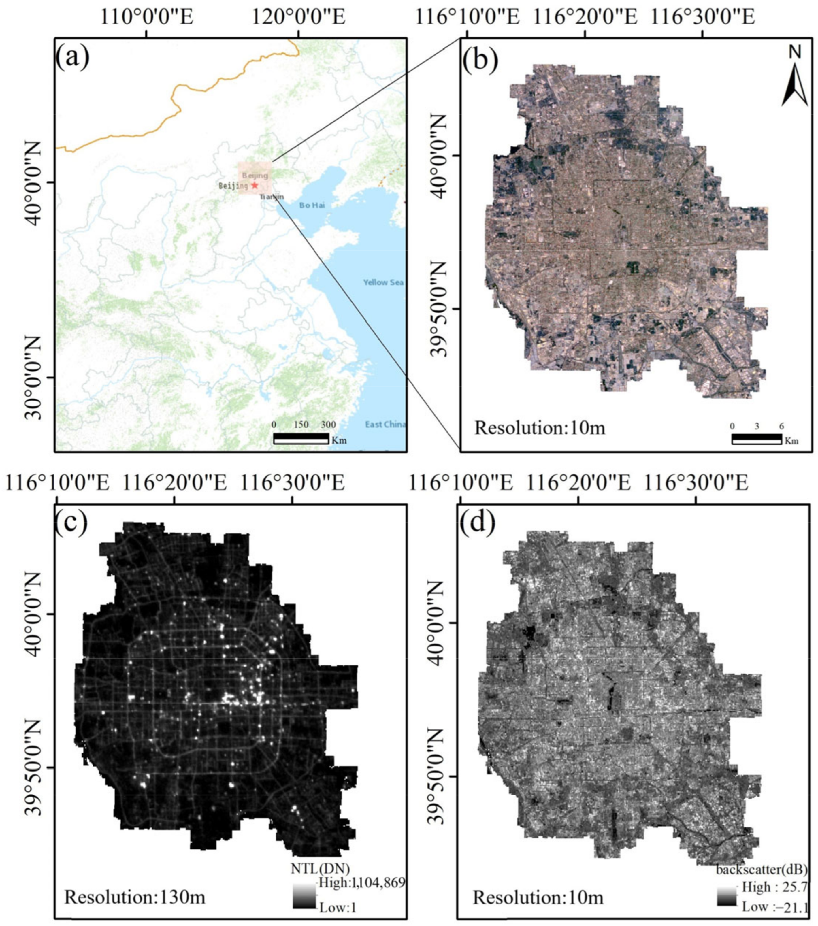
2.1. Study Area

Our study area is Beijing (39°28′–41°05′N, 115°25′–117°30′E), which is the capital city of China (Figure 1). Beijing has a typical warm temperate, semi-humid continental monsoon climate, with hot and rainy summers and cold and dry winters [43]. With rapid urbanization in recent years, built-up land in urban areas has increased dramatically. As a result, building types of LCZs account for a relatively large proportion of the total area within Beijing’s Fifth Ring Road, of which open low-rise and mid-rise buildings with high traditional and cultural architectural value are two essential types of manufactured built LCZs in Beijing [44].

2.2. Data

The primary data selected includes Sentinel-1 SAR, Sentinel 2 Multispectral Instrument (MSI), NTL data, and Landsat-8 Operational Land Imager (OLI) data. Details concerning satellite parameters can be found in

Table 1. Satellite parameters of Sentinel 1A, Sentinel 2A, Luojia-01, and Landsat-8 imageries.

Remotely Sensed Data	Acquire Time	Orbit Altitude (km)	Swath Width (km)	Spatial Resolution (m)	Wavelength
Sentinel-1A Level-1 Ground Range Detected (GRD)	30 November 2018;	693	Interferometric wide swath: 250	Interferometric wide swath: 5 × 20	C-band (5.405 GHz)
	18 November 2018;
	23 November 2018;
	5 December 2018;
Sentinel-2A MSI L2A	8 April 2018; 29 November 2018;	786	290 × 290	10, 20, 60	Coastal aerosol band: 443 nm
					Blue band: 490 nm
					Green band: 560 nm
					Red band: 665 nm
					Vegetation Red Edge-1 band: 705 nm
					Vegetation Red Edge-2 band: 740 nm
					Vegetation Red Edge-3 band: 783 nm
					Near Infrared (NIR) band: 842 nm
					Narrow NIR band: 865 nm
					Water vapor band: 940 nm
					Shortwave infrared (SWIR)-Cirrus band: 1375 nm
					SWIR-1 band: 1610 nm
					SWIR-2 band: 2190 nm
Luojia1-01	Average for the year 2018	634	260 × 260	130	480–800 nm
Landsat-8	Average for the year 2018	703	185 × 185	15, 30, 100	Coastal/Aerosol band: 435–451 nm
					Blue band: 452–512 nm
					Green band: 533–590 nm
					Red band: 636–673 nm
					NIR band: 851–879 nm
					SWIR-1 band: 1566–1651 nm
					SWIR-2 band: 2107–2294 nm
					Pan band: 503–676 nm
					Cirrus band: 1363–1384 nm
					Thermal infrared (TIR)-1 band: 10,600–11,190 nm
					TIR-2 band: 11,500–12,510 nm

.

• Sentinel-1 Synthetic aperture radar:

A dual-polarization C-band SAR instrument produces Sentinel-1 SAR data at 5.405 GHz. Each Sentinel-1 imagery was preprocessed using the Sentinel-1 Toolbox on the Google Earth Engine (GEE) platform, including thermal noise removal, radiometric calibration, and terrain correction. We used the Level-1 GRD product with a spatial resolution of 10 m to calculate the median values for the leaf-on and leaf-off imageries;

• Sentinel-2 Multispectral Instrument:

Sentinel 2 MSI level-2A imageries (atmospheric bottom reflectance) covering the study area were chosen from the GEE platform (Figure 1b). In addition, leaf-on and leaf-off imageries acquired in 2018 were used to help LCZ mapping. Note that Sentinel-2 has a total of 13 bands that can cover visible and near-infrared (VNIR) to SWIR spectrum, and their spatial resolution are 10 m, 20 m, and 60 m [45];

• Night-time light data:

The NTL data records artificial lights on Earth’s surfaces at night, and it is closely related to socioeconomic developments, such as population densities [46]. We used the NTL data from the Luojia1-01 satellite with a spatial resolution of 130 m. Luojia1-01 is the world’s first dedicated NTL satellite, successfully launching on 2 June 2018. Compared with traditional NTL satellites, the new data has a finer spatial resolution with few blooming phenomena;

• Landsat-8 Operational Land Imager data:

Currently, LST is widely used in urban climatology, and the LCZ classification scheme can illustrate the thermal characteristics of underlying surfaces [47]. Therefore, we used the Statistical Mono-Window (SMW) algorithm to retrieve LST in Beijing in 2018 [48]. Notably, the mapping procedure is driven by multi-source remotely sensed imageries with different spatial resolutions, i.e., Sentinel 1A/2A, Landsat-8 OLI data, and Luojia-01 NTL data. To guarantee the consistency concerning spatial details of all data, we adopted bilinear interpolation and pan-sharped methods to project the spatial resolution of multi-source remotely sensed data to 10 m.

2.3. Overview of the Approach

Figure 2 shows the workflow of the LCZ classification. The main idea is to fully use the advantages of daytime and night-time satellite observations and spectral differences in seasonal satellite detection, especially for vegetation phenology. In detail, daytime features were characterized by object spectrums, textures, and surface thermal environments. At night, human activity intensities revealed by light radiation were utilized in the classification procedure. In addition, vertical features of objects, i.e., surface roughness and a backscatter index retrieved by Sentinel-1A SAR, were employed to support the classification.

In addition, feature optimization was conducted utilizing the Gini index (GI) to improve classification accuracy. Furthermore, the RF model was adopted based on the best feature combination to determine the final classification. Finally, in order to evaluate the influence of varying feature categories on the classification, we designed a series of control experiments under four scenarios, i.e., surface roughness vs. no surface roughness, night-time feature vs. no night-time feature, surface thermal feature vs. no surface thermal feature, and leaf-on vs. leaf-off spectrums.

2.4. Sample Preparation

The city block was regarded as the basic spatial unit used to conduct LCZ classification, generated upon the street network’s account. The reference of LCZ classification results was obtained through visual interpretation referring to Google Earth images. Additionally, the reference data is well in line with the LCZ mapping results conducted by Quan et al. [49], suggesting the reliability of our samples.

According to Stewart and Oke [4], we identified 15 LCZ categories, including LCZs 1–10 for artificial systems with a mixture of landscapes that generate by human-environmental interactions, and LCZ A/B-G for natural systems with landscapes that feature little human interference.

Table 2. Samples utilized for the classification.

LCZ Type	The Number of Verification Samples	The Number of Training Samples	The Number of Total Samples
1	13	52	65
2	23	94	117
3	12	46	58
4	98	393	491
5	124	496	620
6	66	265	331
7	2	9	11
8	36	147	184
9	76	304	380
A/B	44	174	218
C	4	11	14
D	327	1310	1637
E	2137	8546	10,683
F	601	2404	3005
G	375	1499	1874

details the samples selected for each LCZ. The training/verification samples were randomly selected using the “model selection” tool provided by the sklearn package. Eighty percent of the samples were chosen to train the classifier, and the others were used to verify the classification accuracy.

Here is a description of the key steps involved in building a random forest classification procedure [50]:

• A sample of N observations is taken with replacement from a dataset. Each observation consists of M attributes;
• When constructing a decision tree, m attributes are randomly chosen from the M attributes at each node, where $m\ll M$. Then, one attribute is selected from the m attributes using a chosen splitting criterion;
• The decision tree is constructed by recursively splitting each node using the selected attribute until it cannot be split any further;
• Repeat steps 1–3 to construct a large number of decision trees, which form the random forest.

2.5. Multi-Feature Extraction

We extracted two feature categories, i.e., daytime features (e.g., surface spectrums, textures, and surface roughness) and night-time features (e.g., NTL radiations), for the subsequent LCZ partition (

Table 3. Multi-feature extraction for LCZ classification.

Category	Feature	Description	References
Spectral feature	Spectral information	B2: Blue band (490 nm)	[51]
		B3: Green band (560 nm)
		B4: Red band (665 nm)
		B5: Vegetation Red Edge-1 band (705 nm)
		B6: Vegetation Red Edge-2 band (740 nm)
		B7: Vegetation Red Edge-3 band (783 nm)
		B8: NIR band (842 nm)
		B8a: Narrow NIR band (865 nm)
		B11: SWIR-1 band (1610 nm)
		B12: SWIR-2 band (2190 nm)
	Normalized difference vegetation index (NDVI)	$\mathrm{NDVI}=\left({\mathrm{B}}_{\mathrm{NIR}}-{\mathrm{B}}_{\mathrm{R}}\right)/\left({\mathrm{B}}_{\mathrm{NIR}}+{\mathrm{B}}_{\mathrm{R}}\right)$	[52]
	Ratio vegetation index (RVI)	RVI = ${\mathrm{B}}_{\mathrm{NIR}}$/${\mathrm{B}}_{\mathrm{R}}$	[53]
	Difference vegetation index (DVI)	DVI = ${\mathrm{B}}_{\mathrm{NIR}}$ − ${\mathrm{B}}_{\mathrm{R}}$	[54]
	Bare soil index (BSI)	$\mathrm{BSI}=\frac{\left({\mathrm{B}}_{\mathrm{R}} + {\mathrm{B}}_{\mathrm{SWIR}}\right) - \left({\mathrm{B}}_{\mathrm{NIR}} + {\mathrm{B}}_{\mathrm{B}}\right)}{\left({\mathrm{B}}_{\mathrm{R}} + {\mathrm{B}}_{\mathrm{SWIR}}\right) + \left({\mathrm{B}}_{\mathrm{NIR}} + {\mathrm{B}}_{\mathrm{B}}\right)}$	[55]
	Normalized difference moisture index (NDMI)	NDWI $=({\mathrm{B}}_{\mathrm{NIR}}$ − ${\mathrm{B}}_{\mathrm{SWIR}}$)/(${\mathrm{B}}_{\mathrm{NIR}}$ + ${\mathrm{B}}_{\mathrm{SWIR}}$)	[56]
	Normalized difference built-up index (NDBI)	NDBI $=({\mathrm{B}}_{\mathrm{MIR}}$ − ${\mathrm{B}}_{\mathrm{NIR}}$)/(${\mathrm{B}}_{\mathrm{MIR}}$ + ${\mathrm{B}}_{\mathrm{NIR}}$)	[57]
	Sentinel-2 red-edge position index (S2REP)	S2REP = 705 + 35 × ((${\mathrm{B}}_{\mathrm{R}}$ + ${\mathrm{B}}_{\mathrm{Vegetation} \mathrm{Red} \mathrm{Edge}1}$)/2 − ${\mathrm{B}}_{\mathrm{Vegetation} \mathrm{Red} \mathrm{Edge}2}$)/(${\mathrm{B}}_{\mathrm{Vegetation} \mathrm{Red} \mathrm{Edge}3}$ − ${\mathrm{B}}_{\mathrm{Vegetation} \mathrm{Red} \mathrm{Edge}2}$)	[58]
	Second brightness index (BI2)	The second Brightness Index algorithm represents the average brightness of a satellite image.	[59]
Thermal infrared information	Land surface temperature (LST)	LST refers to the Earth’s skin temperature.	[60]
Textural feature	Contrast	The contrast derived from GLCM and Grey Level Difference Vector (GLDV).	[61]
	Correlation	The gray correlation derived from GLCM.
	Entropy	The entropy derived from GLCM and GLDV.
	Variance	The variance derived from GLCM.
	Angular second moment	The angular second moment derived from GLCM and GLDV.
	Homogeneity	The homogeneity derived from GLCM.
	Dissimilarity	The heterogeneity parameters derived from GLCM.
Surface roughness	Digital elevation model (DEM)	DEM is the digital representation of the land surface elevation concerning any reference datum.	[62]
	Backscatter (σ)	${\mathsf{\sigma }}^0 = \mathrm{f}(\mathrm{Roughness},\mathrm{Moisture},\mathrm{Geometry},$ $\mathrm{Look} \mathrm{angle},\mathrm{Polarization})$	[63]
NTL	Total night-time light index (TNLI)	$\mathrm{TNLI}=\frac{1}{\mathrm{n}}{\displaystyle {\displaystyle \sum }_{\mathrm{i}=1}^{\mathrm{n}}}{\mathrm{DN}}_{\mathrm{i}}$	[64]

where ${\mathrm{B}}_{\mathrm{R}}$, the surface reflectance of the red band; ${\mathrm{B}}_{\mathrm{NIR}}$, the surface reflectance of the near-infrared band; ${\mathrm{B}}_{\mathrm{SWIR}}$, the surface reflectance of the shortwave infrared band; ${\mathrm{B}}_{\mathrm{B}}$, the surface reflectance of the blue band; ${\mathrm{B}}_{\mathrm{MIR}}$, the surface reflectance of the mid-infrared band; ${\mathrm{B}}_{\mathrm{Vegetation} \mathrm{Red} \mathrm{Edge}1}$, the surface reflectance of the vegetation red edge-1 band; ${\mathrm{B}}_{\mathrm{Vegetation} \mathrm{Red} \mathrm{Edge}2}$, the surface reflectance of the vegetation red edge-2 band; ${\mathrm{B}}_{\mathrm{Vegetation} \mathrm{Red} \mathrm{Edge}3}$, the surface reflectance of the vegetation red edge-3 band; ${\mathrm{DN}}_{\mathrm{i}}$, the light radiance for each raster grid in the region; and $\mathrm{n}$, the number of raster cells in the region.

). Spectral features include a total of 13 spectrums and indices detected by Sentinel satellite (e.g., red, blue, green, and near-infrared bands), normalized difference vegetation index (NDVI), ratio vegetation index (RVI), difference vegetation index (DVI), bare soil index (BSI), normalized difference moisture index (NDMI), normalized difference built-up index (NDBI), Sentinel-2 red-edge position index (S2REP), and second brightness index (BI2). Thermal environments primarily refer to LST retrieved using Landsat-8 thermal infrared band. Texture features are revealed by varying Gray Level Co-occurrence Matrix (GLCM) indices, e.g., angular second moment, variance, contrast, and entropy. Surface roughness, including the digital elevation model (DEM) and backscatter, was generated by Sentinel-1 SAR images. In particular, the total night-time light index (TNLI) was chosen to represent the night-time feature.

2.6. Feature Optimization

The classification accuracy can be significantly improved by distinct cognition and understanding each feature’s importance. To measure the significance of each variable, we introduce the GI, which refers to the probability of an individual feature being incorrectly classified when randomly selected, and the index is a by-product of the RF model [65,66]. Assuming that there are K LCZ types, the probability of a spatial unit belonging to the k-th LCZ is $p_k$; then the definition of the GI is [67]:

$$Gini\left(P\right)={\displaystyle \sum }_{k=1}^K{p}_k\left(1-p_k\right)=1-{\displaystyle \sum }_{k=1}^K{p}_k^2$$

(1)

It is noteworthy that the GI value can be used as a standard to measure the importance of variables. The larger the GI value, the more influential the variable is.

2.7. The Chosen Classifier

It has been proved that the RF classifier often has better classification results than other classifiers [68]. Thus, the RF algorithm was adopted to determine the classification. The RF model can be regarded as a typical supervised machine-learning algorithm that uses multiple decision trees. It randomly creates a set of trees utilizing the training dataset to select a subset and then collects votes under varying trees to predict the results. It yields excellent classification accuracy, evaluates the feature importance, and features good generalization ability [69].

2.8. Experimental Design

To further analyze the importance of each feature and its impact on LCZ classification, we designed a total of 12 experiments under 5 scenarios (

Table 4. Experiments used for LCZ (note that BFC means best feature combination, and the BFC includes features such as DEM, backscatter, and surface thermal characteristic).

Scenario 1	Evaluating the Influence of DEM on the Classification
Experiment	Exp. a	Exp. b	Exp. c
Description	Only DEM	BFC (including DEM)	BFC without DEM
Scenario 2	Evaluating the influence of backscatter on the classification
Experiment	Exp. d	Exp. b	Exp. e
Description	Only backscatter	BFC (including backscatter)	BFC without backscatter
Scenario 3	Evaluating the influence of night-time on the classification
Experiment	Exp. f	Exp. b	Exp. g
Description	Only NTL	BFC (including NTL)	BFC without NTL
Scenario 4	Evaluating the influence of surface thermal feature on the classification
Experiment	Exp. h	Exp. b	Exp. i
Description	Only LST	BFC (including LST)	BFC without LST
Scenario 5	Evaluating the influence of leaf-on and -off on the classification
Experiment	Exp. g	Exp. k	Exp. l
Description	Leaf-on surface spectrum	Leaf-off surface spectrum	Integrating leaf-on and leaf-off surface spectrums

). Experiments a, b, and c in scenario 1 were utilized to evaluate the consequence of DEM on LCZ partitioning. Experiment a used the individual DEM to determine LCZ classification. Experiment b considered the best feature combination (BFC) to complete LCZ mapping. Experiment c was organized to evaluate the impact of the BFC that excludes DEM on LCZ mapping. Experiments d, b, and e in scenario 2 evaluated the influence of backscatter on LCZ classification. Among them, Exp. d utilized the single backscatter feature to determine LCZ mapping, while Exp. e used the BFC that removes backscatter. Experiments f, b, and g in scenario 3 were conceived to assess the distinctive role of night-time observation in LCZ classification. Experiment f utilized only night-time light intensity to label LCZs; in contrast, Experiment g aimed to determine the influence of the BFC without NTL on LCZ partitioning. Experiments h, b, and i in scenario 4 verified the consequence of surface thermal dynamics on LCZ mapping. Experiment h was designed to evaluate the effect of the single LST on LCZ labeling; in contrast, Experiment i assessed the influence of the BFC without LCZ on LCZ classification. In scenario 5, Experiments g and k employed single leaf-on and -off surface spectrums to conduct LCZ mapping, while Exp. l evaluated the fusion effect of leaf-on and -off surface spectrums on LCZ labeling.

2.9. Classification Accuracy Evaluation

After the classification, we need to evaluate the accuracy of LCZ classification. The confusion matrix was employed for accuracy verification [70,71]. Three indicators were utilized to measure the accuracy of the classification results, i.e., OA, PA, and User Accuracy (UA):

$$\left\{\begin{array}{c}\begin{array}{c}OA=\frac{1}{N}{\displaystyle {\displaystyle \sum }_{i=1}^n}{x}_{ii}\\ UA=\frac{x_{ii}}{{{\displaystyle \sum }}_{i=1}^n{x}_{ki}}\\ PA=\frac{x_{ii}}{{{\displaystyle \sum }}_{i=1}^n{x}_{ik}}\end{array}\end{array}\right.$$

(2)

where $n$ is the number of classification categories, $N$ is the total number of samples, $x_{ii}$ is the number of correctly classified samples in the $i$-th category, $x_{ik}$ is the total number of true references in the $i$-th category, and $x_{ki}$ is the pixels in the $i$-th category of the entire image.

3. Results

3.1. Results of Feature Optimization

Figure 3 shows the importance ranking of the chosen variables from high to low involved in LCZ mapping. As shown, TNLI exerted the most influence on the LCZ partition and reached the highest GI value of 0.083. It suggests the importance of night-time satellite observation to enhance LCZ mapping. Backscatter in leaf-on seasons (LN_BS, GI value = 0.029) and backscatter in leaf-off seasons (LF_BS, GI value = 0.025) were found to significantly affect LCZ classification, indicating the critical role of surface roughness in LCZ labeling. Additionally, it was found that some vegetation indices in leaf-off seasons, e.g., RVI and DVI, yielded significant influence on LCZ classification (GI values were higher than 0.02). Additionally, the spectral band (i.e., B12: SWIR-2 band, GI value = 0.021), vegetation index (i.e., DVI in leaf-off seasons, GI value = 0.020), and textural feature in leaf-off seasons (i.e., GLCM correlation) had significant influences on LCZ mapping. Notably, low GI values of some spectral bands in leaf-off seasons were observed, e.g., B6: Vegetation Red Edge-2 band (GI value = 0.013) and B7: Vegetation Red Edge-3 band (GI value = 0.013).

Since feature categories (e.g., textural and spectral features) consist of multiple variables, it is essential to discover the most vital variables in each category. Figure 4 provides the variable importance results for different feature categories. Figure 4a shows that the most critical variable in surface roughness is backscatter in leaf-on seasons (LN_BS, GI value = 0.029), followed by backscatter in leaf-off seasons (LF_BS, GI value = 0.025) and DEM (GI value = 0.017). It indicates that the performance of backscatter is more potent than that of DEM in the LCZ classification. Figure 4b shows the variable importance of textural features. In textural-related features, correlation in leaf-off seasons (LF_Correlation, GI value = 0.021) and correlation in leaf-on seasons (LN_Correlation, GI value = 0.021) yielded good performance in LCZ mapping. In contrast, low GI values of homogeneity in leaf-on seasons (LN_Homogeneity) and dissimilarity in leaf-on seasons (LN_Dissimilarity) were observed, suggesting few influences of LN_Homogeneity and LN_Dissimilarity on LCZ mapping.

Figure 4c provides the variable importance of spectral features in leaf-on seasons. As shown, RVI (GI value = 0.021) and DVI (GI value = 0.020) had noticeable effects on LCZ classification, suggesting vegetation indices in leaf-on seasons is essential to conduct LCZ mapping. However, the effects of B6: Vegetation Red Edge-2 band (GI value = 0.013) and B7: Vegetation Red Edge-3 band (GI value = 0.013) were not evident on LCZ classification. Figure 4d shows the variable importance of spectral features in leaf-off seasons. As shown, B12: SWIR-2 band (GI value = 0.021) and B11: SWIR-1 band (GI value = 0.018) had significant influences on LCZ classification. In contrast, few influences of B6: Vegetation Red Edge-2 band (GI value = 0.013) and B7: Vegetation Red Edge-3 band (GI value = 0.013) were observed on LCZ classification.

To encounter the best combination of LCZ classifications, we calculated OA values under different numbers of input variables (Figure 5). As shown in Figure 5, an increasing trend in OA value was observed with the rising number of input variables. Notably, when the number of input variables reached the threshold (i.e., 29), the highest OA value was observed (88.86%). Additionally, the OA value stood stable with the number of input variables >29. Therefore, considering the accuracy of LCZ classification and computational efficiency, we selected the 29 variables involved in LCZ mapping (Table S3 details the 29 chosen variables).

3.2. Results of LCZ Labeling

Table 5. RF Classification in LCZ for accuracy evaluation (OA, PA, and UA represent overall accuracy, producer’s accuracy, and user’s accuracy, respectively).

LCZ Category	Accuracy Assessment (%)
	PA	UA
LCZ 1	89.1	90.7
LCZ 2	90.6	92.1
LCZ 3	93.0	93.0
LCZ 4	90.2	91.1
LCZ 5	90.6	90.1
LCZ 6	90.2	90.7
LCZ 7	89.3	92.6
LCZ 8	90.6	92.1
LCZ 9	91.8	92.8
LCZ A/B	89.7	91.4
LCZ C	89.6	90.5
LCZ D	88.2	89.9
LCZ E	90.1	88.4
LCZ F	87.3	87.7
LCZ G	88.1	88.2
OA	88.86%

shows the LCZ classification accuracy using the RF classifier with an OA value of 88.86% (Table S4 details the confusion matrix for the BFC). LCZ 3 (compact low-rise) had the best classification result, with PA and UA values exceeding 93%. The possible reason is that DEM, spectral features, and textural features in the compact low-rise type were highly different compared with other climatic zones, leading to the better recognition effect of LCZ 3. On the other hand, LCZ F (bare soil or sand) with PA value = 86.6% and OA value = 87.7% yielded the worst classification effect. The possible reason is that LCZ F and LCZ E (bare rock or paved) share the same texture features and have similar DEM distribution, leading to misclassification between the two LCZ types. It was also found that LCZs 1–10 (artificial systems) yielded better classification results than LCZs A-G (natural systems). The possible reason is significant differences in NTL values between LCZs 1–10. However, natural landscapes in LCZs A-G had few night lights. Moreover, significant differences in buildings’ DEM and thermal environments in LCZs 1–10 were found.

Figure 6 provides classification details revealed by the RF model. Traditional and modern buildings were intermingled, juxtaposed, and mixed in functional core areas due to historical and social reasons, resulting in a complex LCZ system in Beijing. High spatial heterogeneity of landscapes and LCZs was observed outside the active core area [44]. It was found that LCZ 5 (open midrise, accounted for 20.59%) reached the highest area proportion, followed by LCZ 6 (open low-rise, 9.23%). The lowest area proportion was LCZ 7 (lightweight low-rise, below 1%). In natural LCZ systems, LCZ E (bare rock or paved) had the largest share of 38.88%, followed by LCZ F (bare soil or sand). In contrast, LCZ C (bush, scrub) yielded the lowest area proportion (less than 1%).

Generally speaking, the accuracy of artificial LCZ classification, i.e., LCZs 1–10, was higher than that of natural LCZ classification, i.e., LCZs A-G (Figure 6d,h). The noted wrong labeling is also shown in Figure 6. LCZ E (bare rock or paved), the white oval (location A) in Figure 6b, was wrongly labeled as LCZ D (low plants) (Figure 6c). Additionally, the blue rectangle (location B) and yellow rectangle (location C) in Figure 6b should be LCZ F (bare soil or sand); however, they were incorrectly identified as LCZ 5 (open midrise) and LCZ 9 (sparsely built) (Figure 6c). Moreover, LCZ F (bare soil or sand), the purple rectangle (location D) and the pink rectangle (location F) in Figure 6f, was wrongly labeled as LCZ 5 (open midrise). The green rectangle (location E) in Figure 6f should be LCZ 5 (open midrise), but it was incorrectly identified as LCZ E (bare rock or paved) in Figure 6g. Our results indicate that bare rock (or paved) and bare soil (or sand) were easy to label as artificial LCZ categories.

3.3. The Consequence of Surface Thermal Properties on LCZ Mapping

LCZ classification scheme was proposed for studies involving urban climates and heat islands. Thus, exploring the consequence of underlying surfaces’ thermal dynamics on LCZ classifications is essential. Figure 7 shows LCZ partitioning results that used single LST, BFC with LST, and BFC without LST. As shown, the OA values of Exp. b (BFC with LST), Exp. i (BFC without LST), and Exp. h (single LST) were 88.86%, 87.66%, and 56.62% (details concerning the confusion matrix of three classifiers are shown in Supplementary Material Tables S4, S11, and S12). It suggests that underlying surfaces’ thermal dynamics can be used to enhance LCZ classification. Notably, the accuracies of LCZs 1–9 were considerably increased when using the LST feature. Among these, the accuracy of LCZ 3 (compact low-rise) significantly increased by 16.10%. The possible reason is that the relative amount of vertically oriented surfaces and the corresponding variations in surface insolation within the built-up area make a significant contribution to the difference in surface temperatures [38,72,73,74]. However, the OA values of LCZs E (bare rock or paved) and F (bare soil or sand) in Exp. b were lower than those in Exp. i. The possible reason is that similar paves with dark-colored materials yielded parallel LST distribution. Asphalt and concrete materials absorb heat from the sun during the day and re-radiate it at night [15,75,76,77].

Figure 8 shows classification results that used single LST, BFC with LST, and BFC without LCZ. As shown, LCZ F (bare soil or sand), i.e., red rectangle (location G) and purple rectangle (location H) in Figure 8, was wrongly labeled as LCZ 5 (open midrise) in Exps. h and b. Nevertheless, it was correctly labeled in Exp. i. The possible reason is that the materials of pavements in urban areas are concrete and asphalt. These materials differ considerably in thermal properties (including heat capacity and thermal conductivity) and surface emissivity (albedo and emissivity) compared with natural environments. Thus, underlying surfaces’ thermal dynamics can improve the accuracy of the LCZ classification [78,79,80]. Additionally, it was found that LCZ A/B (dense trees) was wrongly classified as LCZ D (low plants) in the experiment (locations I and J) that did not use the LST feature. In contrast, it was correctly labeled in the experiments that used the LST feature. The possible reason is that a large difference in surface temperature existed between LCZs A/B and D since the vegetation proportion and radiative response of bare soils can significantly influence surface temperature variations [7,39,40,60].

3.4. The Distinctive Role of Night-Time Observations in LCZ Mapping

It is primarily known that night-time satellite observations can detect artificial lights from Earth’s surfaces, which represent human activities, economic levels, and anthropogenic heat flux (AHF). Therefore, this study systematically analyzed how NTL data influence LCZ labeling. Figure 9 illustrates the overall accuracy of classification results that used single NTL, BFC with NTL, and BFC without LCZ. It was found that Exp. b (BFC with NTL, OA value = 88.26%) yielded the highest accuracy of LCZ labeling, followed by Exp. g (BFC without NTL, OA value = 85.41%) and Exp. f (single NTL, OA value = 55.45%) (details concerning the confusion matrix of three classifiers are shown in Supplementary Materials Tables S4, S9, and S10). When using night-time observations, the accuracy of LCZs 1–9 (artificial landscapes) was significantly improved. In addition, the accuracy of natural LCZ settings (i.e., LCZs A–G) slightly increased after adding the NTL feature to the classification procedure. The possible reason is that NTL data overcomes the shortcomings of Sentinel-2 optical imageries in terms of shading effects of buildings, bridges, and towers in artificial LCZs, and the shading effects are not evident in natural LCZ settings [81,82,83]. It is noteworthy that NTL largely contributed to the classification concerning LCZ 3 (compact low-rise) and LCZ A/B (dense trees), which is well in line with Qiu et al. [31]. Higher NTL was found in the center of the city (i.e., LCZ 3), while lower NTL was observed in the peripheral areas of the city characterized by natural environments (i.e., LCZ A/B) [83]. NTL is useful in classifying artificial LCZs, probably owing to a high correlation between NTL and building vertical information. Building heights or volumes usually increase as NTL values rise [84,85].

To better illustrate the consequence of the NTL variable on LCZ classification, we designed a set of comparative experiments (Figure 10). LCZ 8 (large low-rise), the blue rectangle (location K) and the yellow rectangle (location L) in Figure 10, was wrongly labeled as LCZ A/B (dense trees) in Exp. g, and it was correctly classified in Exps. f and b. It may be due to NTL representing impervious surface coverages that can be used to distinguish urban regions from non-urban surfaces (e.g., forests, vegetation, and water bodies) [86,87,88,89]. Additionally, the red (location N) and white (location M) rectangles in Figure 10 were accurately classified as LCZ 4 (open high-rise) in Exps. f and b, while they were wrongly labeled as LCZ 5 (open midrise) in Exp. g. It can be attributed to the fact that optical imageries rely on sunlight as the source of illumination for intensity detection, which would cast shadows on some underlying surfaces, leading to misclassification and errors. NTL can address the questions related to shadows [81,90].

Based on this, it can be seen that night-time light remote sensing data can not only obtain surface cover information by fusing other daytime remote sensing data, but also analyze human activity areas with its own special information collection capabilities. Therefore, night-time light remote sensing data has received increasing attention. Qiu et al. [31] combined day and night data and used a residual convolutional neural network method to analyze the feature importance of nine European cities. The results showed that NTL can improve the classification accuracy of LCZ samples. Cai et al. [91] used urban form data, landscape indicators, night-time light images, and fine-resolution annual fixed effects models in LCZ to simulate the spatiotemporal carbon emissions of the Yangtze River Delta and the Pearl River Delta in China. The results showed that this method accurately extracted urban areas and could more clearly identify changes in carbon emissions within cities. Therefore, combining daytime and night-time data analysis is essential. Chung et al. [81] proposed using the optimal data and Machine Learning Algorithm on the Google Earth Engine platform to generate large-scale LCZ maps. The research results showed that VIIRS night-time light data has significant LCZ classification potential.

4. Discussion

4.1. How Does Surface Roughness Impact the LCZ Classification?

4.1.1. The Advantages of DEM for the Classification

Since the LCZ scheme considers two-dimensional and three-dimensional urban structure parameters, it is essential to evaluate how surface roughness impacts LCZ classification [4]. Figure 11 compares LCZ classification results using single DEM, BFC with DEM, and BFC without DEM (details concerning the confusion matrix of three classifiers are shown in Supplementary Materials Tables S4–S6). As shown, Exp. b (i.e., BFC with DEM) had the highest accuracy with an OA value of 86.72%, followed by Exp. c (i.e., BFC without DEM) with an OA value of 82.35%. As expected, Exp. a (i.e., single DEM) with an OA value of 61.83% yielded the lowest accuracy. DEM feature can improve the experimental accuracy by 2.14%, indicating numerous advantages of integrating DEM to enhance LCZ labeling. It was found that DEM can significantly improve the accuracy of the labeling regarding LCZs 1–6 (compact and open buildings) and LCZ A/B (dense trees). In contrast, DEM did not help the classifications concerning LCZ 8 (large low-rise) and LCZs C-G. Given that the LCZ classification scheme is related to three-dimensional urban structure parameters [47,92], DEM information can be beneficial for distinguishing LCZs with varying building heights (i.e., LCZs 1–3 and LCZs 4–6) and for identifying dense trees from natural landscapes, i.e., LCZ A/B (dense trees). However, the improvement of DEM on LCZs with scattered trees, i.e., LCZs 6, 9, B, and C, was not evident [22,93]. It is primarily known that identifying the three-dimensional characteristics of underlying surfaces is still a challenge for optical spectral imageries since buildings featuring high-rise, medium-rise, and low-rise would yield similar spectral information [31,94]. Thus, it is of importance to use the roughness model to help LCZ classification.

Figure 12 shows the analytic results regarding LCZ classification in Exps. a (using single DEM), b (using BFC with DEM), and c (using BFC without DEM). As shown, the yellow oval (location P) in Figure 12 should be LCZ F (bare soil or sand); however, it was wrongly classified as LCZ 6 (open low-rise) in Exps. a and b. Moreover, the green rectangle (location S) in Figure 12 should be LCZ F (bare soil or sand), but it was misclassified as LCZs 8, D, and F in Exps. a, b, and c, respectively. It indicates that DEM may confuse LCZ F (bare soil or sand) with other LCZ systems featuring similar elevation distribution. In addition, the blue rectangle (location O) in Figure 12 was misclassified as LCZ E (bare rock or paved) in Exp. c that used BFC without the DEM, and it was correctly labeled as LCZ 9 (sparsely built) in Exps. a and b that used BFC with the DEM. LCZ 9 with sparse buildings is very similar to natural landscape settings, and our finding suggests that high-resolution Interferometric synthetic aperture radar (InSAR)-derived DEM helps capture buildings sparsely. LCZ 5 (open midrise) was wrongly labeled as LCZ E (bare rock or paved) in Exp. c (the white rectangle (location Q) in Figure 12); however, it was correctly identified in Exps. a and b. It suggests that DEM can be significantly helpful in labeling midrise buildings. Our experimental results also indicate that adding DEM is beneficial for the classifications regarding LCZ 5 (open midrise, the white rectangle (location Q) in Figure 12) and LCZ 8 (large low-rise, the purple rectangle (location R) in Figure 12).

4.1.2. The Advantages of Backscatter for the Classification

Figure 13 shows LCZ classifications revealed by Exps. b, d, and e. Exp. b, which used BFC with backscatter, yielded the highest accuracy with an OA value of 88.86%, followed by Exp. e that used BFC without backscatter with an OA value of 85.84%. The lowest accuracy of the LCZ classification was Exp. d that used single backscatter with an OA value of 70.06% (details concerning the confusion matrix of three classifiers are shown in Supplementary Materials Tables S4, S7, and S8). The results show that the backscatter feature increased the OA value by 3.02%. SAR systems record the amplitude and phase of the backscattered signal, which largely depends on the physical of the imaged object (e.g., terrain roughness). Thus, backscatter can somewhat reflect object surface roughness [95,96,97]. Bechtel et al. [98] have demonstrated that backscatter is the most important feature of dividing most artificial landscapes from natural environment settings. As shown, LCZs 1–6 (compact and open buildings) in Exp. b that used BFC with backscatter yielded higher classification accuracy compared with that in Exp. e that used BFC without backscatter. It can be attributed to the fact that buildings in built-up areas tend to be taller and more evident, thus producing stronger backscatter [99,100]. However, it was found that adding backscatter decreased the classification accuracy of LCZs 7 (lightweight low-rise) and 8 (large low-rise). It is because of the fact that some small buildings may suffer from signal loss due to multiple bounces and that the average value of backscatter from wooden building materials exceeds only 1–2 dB compared to backgrounds [99]. Although backscatter is powerful in distinguishing between urban and non-urban LCZ settings, the confusion between LCZs 3 (compact low-rise) and 8 (large low-rise) was observed when using backscatter. It is well in line with an investigation regarding the use of SAR data on LCZ partitioning based upon WUDAPT conducted by Bechtel et al. [98]. In spite of complex and diverse building materials and layouts, backscatter tends to be similar for buildings sharing similar heights [101]. Backscatter information is responsive to vertical features of underlying surfaces [81,102,103], and our experiments have demonstrated that backscatter is useful for the distinction between urban and rural environments. The analytic experiments also show that the holistic use of backscatter and DEM information is essential for the fine classification of LCZ.

Figure 14 shows the classification results that used single backscatter, BFC with backscatter, and BFC without backscatter. The white rectangle (location T) was correctly labeled as LCZ 9 (sparsely built) in both Exps. d and e. At the same time, it was wrongly labeled as LCZ 6 (open low-rise) in Exp. b. This indicates that backscatter incorporating other features may misclassify LCZ 9 (sparsely built) to LCZ 6 (open low-rise). On the other hand, LCZ F (bare soil or sand), the green oval (location U) in Figure 14, was wrongly labeled as LCZ 9 (sparsely built) in Exp. d, and it was correctly classified in Exps. e and b. The possible reason is that LCZ 9 is an underlying composite surface consisting of sparse and residential buildings, which tend to be confused with LCZs 5 (open mid-rise) and F (bare soil or sand) categories because of the similarity of roof materials [99]. Moreover, in complicated LCZ settings (i.e., yellow rectangle (location W) and purple rectangle (location V) in Figure 14), the classification performances of Exps. d and b were better than those of Exp. e. It suggests that backscatter can enhance LCZ labeling. The possible reason is that vertical information of underlying surfaces can help with urban scene understanding and largely reflect the intensity of human activity [73,104].

4.2. Synergetic Use of Leaf-On and -Off Imageries

Surface reflectance has been extensively used to conduct underlying surface classification and urban scene understanding [105,106,107]. In addition, there are varying seasonal cycles of surface reflectance because of changing solar altitude angles and vegetation phenology [108,109,110]. Thus, the synergetic use of leaf-on and -off imageries can, to some extent, help LCZ classification. As shown in Figure 15, significant differences in the average surface reflectance of each LCZ were observed. In addition, the reflectance of vegetation in leaf-off seasons was considerably lower than that in leaf-on seasons, and the reflectance of the green band (band 3) was approximately 10% in leaf-on seasons and <10% in leaf-off seasons. Our results demonstrate that the synergetic use of leaf-on and -off imageries may provide more spectral information for LCZ mapping and can help in the identification of LCZ settings [111,112].

Figure 16 compares LCZ classification results using leaf-on imageries, leaf-off imageries, and integrating leaf-on and leaf-off imageries. It was found that Exp. l (blending leaf-on and leaf-off imageries, OA value = 63.49%) yielded the highest accuracy of LCZ labeling, followed by Exp. k (single leaf-off imagery, OA value = 59.87%) and Exp. j (single leaf-on imagery, OA value = 58.74%) (details concerning the confusion matrix of three classifiers are shown in Supplementary Materials Tables S13–S15). It is consistent with the conclusions of Zhao et al. [113] that the reflectance in leaf-off seasons was observed to be more advantageous than that in leaf-on seasons in the scene understanding and underlying surface classification. Notably, the performance of integrating leaf-on and -off imageries was better than the single use of any of those (the OA value increased by 4.75% compared with the single use of leaf-on imagery and 3.62% than that of leaf-off imagery).

Figure 17 shows the classification results that used leaf-on, leaf-off, and combined leaf-on and -off imageries. LCZ D (low plants), white rectangle (location X), and blue rectangle (location Y) in Figure 17 were wrongly classified as LCZ F (bare soil or sand) in Exp. k and LCZ A/B (dense trees) in Exp. j. However, it was correctly classified in Exp. l. We have demonstrated that the blending of leaf-on and -off imageries provides more accurate classification results than the single use of any of these. The possible reason is the vegetation phenology, e.g., trees in leaf-on seasons have a high abundance, whereas vegetation may evolve bare soils in leaf-off seasons [72,114]. Our results demonstrated that seasonal changes in surface reflectance are vital for LCZ labeling; this is particularly true when considering the rapid land use changes because of agricultural activities [115,116].

4.3. Comparison with Considerable Methods

To better illustrate the advantages of the proposed method, we compared it with numerous methods that used satellite imageries with a medium spatial resolution (i.e., higher than a 10 m spatial resolution) from the perspectives of data sources and results in accuracy (

Table 6. The comparison between the proposed method and existing methods.

Method	Data Source	Study Area	Accuracy (the OA Value)
Random forest classifier and grid-based method [22]	Sentinel-2 (10 m) and Phased Array type L-band Synthetic Aperture Radar-2 (PALSAR-2) (10 m)	Nanchang, China	89.96%
Residual convolutional neural network [31]	Sentinel-2 images (10 m), Landsat-8 image (10 m), Global Urban Footprint (GUF), NTL, and OpenStreetMap (OSM)	Cities in Europe	72–78%
Convolutional neural network [94]	Sentinel-2A/B images and DEM (90 m)	Cities in Germany	86.5%
Multi-scale and multi-level attention network [21]	Sentinel-2 images (10 m), OSM (building footprint data), ALOS World 3D—30m (AW3D30) Digital Surface Model (30 m), and Level-2 national land cover map	Cities in South Korea	~80%
Deep learning method [9]	Sentinel-2 images (10 m, 20 m) and Reference data (Google Earth)	Cities in China	88.61%
Deep learning model [118]	Sentinel-2 images (10 m), Landsat-8 images (30 m), NLI (750 m), Road density (RD) (100 m), Population density (POP) (100 m) and LST data (30 m)	Wuhan, China	74.56%
Proposed method	Sentinel 1/2A imageries at both leaf-on and -off seasons (10 m), high-resolution NTL data (130 m), and Landsat LST data (10 m)	Beijing, China	88.86%

). It is noteworthy that the LCZ classification criterion considers 2D and 3D urban structures, covers, and human activities, and it can be used as a critical indicator for revealing surface urban heat islands or urban climates. Therefore, it is essential to integrate multi-source remotely sensed imageries that consider multiple different features to enhance LCZ classification. Firstly, our method evaluates the consequence of surface thermal properties, i.e., using LST, on LCZ labeling (Table 6), which has rarely been reported in previous literature. Scholars have demonstrated that the LCZ classification scheme is helpful for comparative analyses of land surface temperature dynamics among different cities and can be valuable for the examination of the evolution of land surface temperatures over time [117]. Conversely, LST can be helpful for the LCZ classification to some extent. Our results demonstrated that the accuracies of LCZs 1–9 were considerably increased when using the LST feature. Among these, the accuracy of LCZ 3 (compact low-rise) significantly increased by 16.10% (Figure 7 and Figure 8). Secondly, our method provides a clear picture of the advantages of the synergetic use of diurnal satellite observation on the LCZ classification. The high spatial resolution NTL data with a spatial resolution of 130-m can largely reflect the intensities of human activities, which is an essential feature of the LCZ classification. In this study, it was found that high spatial resolution NTL occupied a high GI value and increased the OA value of the classification by 3.44% (Figure 9). Finally, our method yielded high classification accuracy, no less than that of most existing methods (Table 6), which also verified the advantages of our methods.

5. Conclusions

In this study, we proposed a new method for LCZ mapping that fully explicates seasonal and diurnal satellite observations and uses the RF classifier. In addition, this study proposes a method that uses a random forest classifier and multi-source remotely sensed data, including Sentinel-1 SAR, Sentinel-2 MSI, and Luojia1-01 night-time light data.

Firstly, multiple features, including spectral and texture features from Sentinel-2 MSI and surface roughness and a backscatter index from Sentinel-1 SAR, were extracted. Additionally, leaf-on and -off imageries and underlying surface thermal features were synergistically used in LCZ mapping. Secondly, the Gini Index was introduced to measure the significance of each feature. At last, we designed six classification scenarios and adopted the RF classifier to complete the labeling and compare the consequence of different input features on the classification accuracy. The conclusions can be drawn as follows.

• The present method yielded excellent classification accuracy with an OA value of 88.86%. LCZ 3 (compact low-rise) had the best classification result, with PA and UA values exceeding 93%. LCZ F (bare soil or sand) with PA value = 86.6% and OA value = 87.7% yielded the worst classification effect. The total night-time light index (TNLI) exerted the most considerable influence on the LCZ partition and reached the highest GI value of 0.083. Backscatter in leaf-on seasons (LN_BS, GI value = 0.029) and backscatter in leaf-off seasons (LF_BS, GI value = 0.025) were found significantly affect LCZ classification;
• The accuracies of LCZs 1–9 were considerably increased when using the LST feature. Among these, the accuracy of LCZ 3 (compact low-rise) significantly increased by 16.10%. NTL largely contributed to the classification concerning LCZ 3 (compact low-rise) and LCZ A/B (dense trees). DEM can significantly improve the accuracies of classifications regarding LCZs 1–6 (compact and open buildings) and LCZ A/B (dense trees). In contrast, DEM did not help the classifications concerning LCZ 8 (large low-rise) and LCZs C-G;
• LCZs 1–6 (compact and open buildings) using BFC with backscatter yielded higher classification accuracy than those using BFC without backscatter. In addition, the performance of integrating leaf-on and -off imageries was better than the single use of any of those (the OA value increased by 4.75% compared with the single use of leaf-on imagery and 3.62% compared with that of leaf-off imagery).

This research is important for the study of LCZ because it evaluates the impact of different feature factors on the accuracy of LCZ classification using multi-source remote sensing data. By understanding the effects of factors such as DEM, backscatter, night-time lights, LST, and growing season on LCZ classification, future researchers and decision-makers can better provide information for urban planning and management decisions, and support climate change research and mitigation efforts. Therefore, this research helps to understand better the complex relationships between climate, land use, and urbanization.

Meanwhile, we can get the relationship between daytime and night-time remote sensing data is significant [119,120]. During the daytime, remote sensing data is typically collected in bands such as visible light and near-infrared, which are highly sensitive to the reflection and radiation of surface objects during the daytime [121]. This makes daytime remote sensing data useful for obtaining high-quality land cover information. At night, remote sensing satellites gather visible and near-infrared electromagnetic wave information emitted from the surface, which primarily reflects human activities on the surface, particularly human night lighting. It can also provide information on the thermal distribution and radiation of the surface and can be used to detect urban lighting information [122,123,124]. Through our experiments, it has been found that combining night-time light data with daytime data can increase the classification accuracy of LCZ, because daytime remote sensing data provides information on land cover types, while night-time remote sensing data provides information on urban lighting distribution. Therefore, the integration of the two datasets leads to a higher level of accuracy in the classification of LCZ.

References

1. Cao, S.S.; Weng, Q.H.; Lu, L.L. Distinctive roles of two- and three-dimensional urban structures in surface urban heat islands over the conterminous United States. Urban Clim. 2022, 44, 101230. [Google Scholar] [CrossRef]
2. Dong, P.; Jiang, S.D.; Zhan, W.F.; Wang, C.L.; Miao, S.Q.; Du, H.L.; Li, J.F.; Wang, S.S.; Jiang, L. Diurnally continuous dynamics of surface urban heat island intensities of local climate zones with spatiotemporally enhanced satellite-derived land surface temperatures. Build. Environ. 2022, 218, 109105. [Google Scholar] [CrossRef]
3. Cao, S.S.; Cai, Y.L.; Du, M.Y.; Weng, Q.H.; Lu, L.L. Seasonal and diurnal surface urban heat islands in China: An investigation of driving factors with three-dimensional urban morphological parameters. GISci. Remote Sens. 2022, 59, 1121–1142. [Google Scholar] [CrossRef]
4. Stewart, I.D.; Oke, T.R. Local climate zones for urban temperature studies. Bull. Am. Meteorol. Soc. 2012, 93, 1879–1900. [Google Scholar] [CrossRef]
5. Bechtel, B.; See, L.; Mills, G.; Foley, M. Classification of local climate zones using SAR and multispectral data in an arid environment. IEEE J. Sel. Top. Appl. Earth Obs. Remote Sens. 2016, 9, 3097–3105. [Google Scholar] [CrossRef]
6. Perera, N.G.R.; Emmanuel, R. A “Local Climate Zone” based approach to urban planning in Colombo, Sri Lanka. Urban Clim. 2018, 23, 188–203. [Google Scholar] [CrossRef]
7. Wang, C.Y.; Middel, A.; Myint, S.W.; Kaplan, S.; Brazel, A.J.; Lukasczyk, J. Assessing local climate zones in arid cities: The case of Phoenix, Arizona and Las Vegas, Nevada. ISPRS J. Photogramm. Remote Sens. 2018, 141, 59–71. [Google Scholar] [CrossRef]
8. Richard, Y.; Emery, J.; Dudek, J.; Pergaud, J.; Chateau-Smith, C.; Zito, S.; Rega, M.; Vairet, T.; Castel, T.; Thévenin, T. How relevant are local climate zones and urban climate zones for urban climate research? Dijon (France) as a case study. Urban Clim. 2018, 26, 258–274. [Google Scholar] [CrossRef]
9. Liu, S.J.; Shi, Q. Local climate zone mapping as remote sensing scene classification using deep learning: A case study of metropolitan China. ISPRS J. Photogramm. Remote Sens. 2020, 164, 229–242. [Google Scholar] [CrossRef]
10. Demuzere, M.; Kittner, J.; Martilli, A.; Mills, G.; Moede, C.; Stewart, I.D.; van Vliet, J.; Bechtel, B. A global map of local climate zones to support earth system modelling and urban-scale environmental science. Earth Syst. Sci. Data 2022, 14, 3835–3873. [Google Scholar] [CrossRef]
11. Han, B.; Luo, Z.X.; Liu, Y.; Zhang, T.Y.; Yang, L. Using Local Climate Zones to investigate Spatio-temporal evolution of thermal environment at the urban regional level: A case study in Xi’an, China. Sustain. Cities Soc. 2022, 76, 103495. [Google Scholar] [CrossRef]
12. Wang, R.; Voogt, J.; Ren, C.; Ng, E. Spatial-temporal variations of surface urban heat island: An application of local climate zone into large Chinese cities. Build. Environ. 2022, 222, 109378. [Google Scholar] [CrossRef]
13. Bechtel, B.; Demuzere, M.; Mills, G.; Zhan, W.; Sismanidis, P.; Small, C.; Voogt, J. SUHI analysis using Local Climate Zones—A comparison of 50 cities. Urban Clim. 2019, 28, 100451. [Google Scholar] [CrossRef]
14. Zhu, Z.; Woodcock, C.E.; Rogan, J.; Kellndorfer, J. Assessment of spectral, polarimetric, temporal, and spatial dimensions for urban and peri-urban land cover classification using Landsat and SAR data. Remote Sens. Environ. 2012, 117, 72–82. [Google Scholar] [CrossRef]
15. Chen, Y.P.; Zheng, B.H.; Hu, Y.Z. Mapping Local Climate Zones Using ArcGIS-Based Method and Exploring Land Surface Temperature Characteristics in Chenzhou, China. Sustainability 2020, 12, 2974. [Google Scholar] [CrossRef]
16. Danylo, O.; See, L.; Bechtel, B.; Schepaschenko, D.; Fritz, S. Contributing to WUDAPT: A local climate zone classification of two cities in Ukraine. IEEE J. Sel. Top. Appl. Earth Obs. Remote Sens. 2016, 9, 1841–1853. [Google Scholar] [CrossRef]
17. Ching, J.; Mills, G.; Bechtel, B.; See, L.; Feddema, J.; Wang, X.; Ren, C.; Brousse, O.; Martilli, A.; Neophytou, M.; et al. WUDAPT An Urban Weather, Climate, and Environmental Modeling Infrastructure for the Anthropocene. Bull. Am. Meteorol. Soc. 2018, 99, 1907–1928. [Google Scholar] [CrossRef]
18. Demuzere, M.; Bechtel, B.; Middel, A.; Mills, G. Mapping Europe into local climate zones. PLoS ONE 2019, 14, e0214474. [Google Scholar] [CrossRef]
19. Demuzere, M.; Hankey, S.; Mills, G.; Zhang, W.; Lu, T.; Bechtel, B. Combining expert and crowd-sourced training data to map urban form and functions for the continental US. Sci. Data 2020, 7, 264. [Google Scholar] [CrossRef]
20. Brousse, O.; Martilli, A.; Foley, M.; Mills, G.; Bechtel, B. WUDAPT, an efficient land use producing data tool for mesoscale models? Integration of urban LCZ in WRF over Madrid. Urban Clim. 2016, 17, 116–134. [Google Scholar] [CrossRef]
21. Kim, M.; Jeong, D.; Kim, Y. Local climate zone classification using a multi-scale, multi-level attention network. ISPRS J. Photogramm. Remote Sens. 2021, 181, 345–366. [Google Scholar] [CrossRef]
22. Ren, C.; Cai, M.; Li, X.; Zhang, L.; Wang, R.; Xu, Y.; Ng, E. Assessment of local climate zone classification maps of cities in China and feasible refinements. Sci. Rep. 2019, 9, 18848. [Google Scholar] [CrossRef]
23. Chen, C.M.; Bagan, H.; Xie, X.; La, Y.N.; Yamagata, Y. Combination of Sentinel-2 and PALSAR-2 for Local Climate Zone Classification: A Case Study of Nanchang, China. Remote Sens. 2021, 13, 1902. [Google Scholar] [CrossRef]
24. Gawlikowski, J.; Schmitt, M.; Kruspe, A.; Zhu, X.X. On the fusion strategies of Sentinel-1 and Sentinel-2 data for local climate zone classification. In Proceedings of the IEEE International Geoscience and Remote Sensing Symposium, Waikoloa, HI, USA, 26 September–2 October 2020; pp. 2081–2084. [Google Scholar]
25. Lu, D.; Weng, Q. A survey of image classification methods and techniques for improving classification performance. Int. J. Remote Sens. 2007, 28, 823–870. [Google Scholar] [CrossRef]
26. Li, N.; Lu, D.S.; Wu, M.; Zhang, Y.L.; Lu, L.Y. Coastal wetland classification with multiseasonal high-spatial resolution satellite imagery. Int. J. Remote Sens. 2018, 39, 8963–8983. [Google Scholar] [CrossRef]
27. Xie, Z.L.; Chen, Y.L.; Lu, D.S.; Li, G.Y.; Chen, E.X. Classification of Land Cover, Forest, and Tree Species Classes with ZiYuan-3 Multispectral and Stereo Data. Remote Sens. 2019, 11, 164. [Google Scholar] [CrossRef]
28. Valjarević, A.; Djekić, T.; Stevanović, V.; Ivanović, R.; Jandziković, B. GIS numerical and remote sensing analyses of forest changes in the Toplica region for the period of 1953–2013. Appl. Geogr. 2018, 92, 131–139. [Google Scholar] [CrossRef]
29. Ju, J.; Kolaczyk, E.D.; Gopal, S. Gaussian mixture discriminant analysis and sub-pixel land cover characterization in remote sensing. Remote Sens. Environ. 2003, 84, 550–560. [Google Scholar] [CrossRef]
30. Yang, J.; Wang, Y.C.; Xiu, C.L.; Xiao, X.M.; Xia, J.H.; Jin, C. Optimizing local climate zones to mitigate urban heat island effect in human settlements. J. Clean. Prod. 2020, 275, 123767. [Google Scholar] [CrossRef]
31. Qiu, C.P.; Schmitt, M.; Mou, L.C.; Ghamisi, P.; Zhu, X.X. Feature Importance Analysis for Local Climate Zone Classification Using a Residual Convolutional Neural Network with Multi-Source Datasets. Remote Sens. 2018, 10, 1572. [Google Scholar] [CrossRef]
32. Yao, X.; Zhu, Z.P.; Zhou, X.W.; Shen, Y.P.; Shen, X.B.; Xu, Z.H. Investigating the effects of urban morphological factors on seasonal land surface temperature in a “Furnace city” from a block perspective. Sustain. Cities Soc. 2022, 86, 104165. [Google Scholar] [CrossRef]
33. Liu, Z.; He, C.; Zhang, Q.; Huang, Q.; Yang, Y. Extracting the dynamics of urban expansion in China using DMSP-OLS nighttime light data from 1992 to 2008. Landsc. Urban Plann. 2012, 106, 62–72. [Google Scholar] [CrossRef]
34. Yu, B.; Shu, S.; Liu, H.; Song, W.; Wu, J.; Wang, L.; Chen, Z. Object-based spatial cluster analysis of urban landscape pattern using nighttime light satellite images: A case study of China. Int. J. Geogr. Inf. Sci. 2014, 28, 2328–2355. [Google Scholar] [CrossRef]
35. Sharma, R.C.; Tateishi, R.; Hara, K.; Gharechelou, S.; Iizuka, K. Global mapping of urban built-up areas of year 2014 by combining MODIS multispectral data with VIIRS nighttime light data. Int. J. Digit. Earth 2016, 9, 1004–1020. [Google Scholar] [CrossRef]
36. Huang, X.; Schneider, A.; Friedl, M.A. Mapping sub-pixel urban expansion in China using MODIS and DMSP/OLS nighttime lights. Remote Sens. Environ. 2016, 175, 92–108. [Google Scholar] [CrossRef]
37. Skarbit, N.; Gál, T.; Unger, J. Airborne surface temperature differences of the different Local Climate Zones in the urban area of a medium sized city. In Proceedings of the Joint Urban Remote Sensing Event (JURSE), Lausanne, Switzerland, 30 March–1 April 2015; pp. 1–4. [Google Scholar]
38. Geletič, J.; Lehnert, M.; Savić, S.; Milošević, D. Inter-/intra-zonal seasonal variability of the surface urban heat island based on local climate zones in three central European cities. Build. Environ. 2019, 156, 21–32. [Google Scholar] [CrossRef]
39. Geletič, J.; Lehnert, M.; Dobrovolný, P. Land surface temperature differences within local climate zones, based on two central European cities. Remote Sens. 2016, 8, 788. [Google Scholar] [CrossRef]
40. Cai, M.; Ren, C.; Xu, Y.; Lau, K.K.-L.; Wang, R. Investigating the relationship between local climate zone and land surface temperature using an improved WUDAPT methodology—A case study of Yangtze River Delta, China. Urban Clim. 2018, 24, 485–502. [Google Scholar] [CrossRef]
41. Brousse, O.; Georganos, S.; Demuzere, M.; Vanhuysse, S.; Wouters, H.; Wolff, E.; Linard, C.; Nicole, P.-M.; Dujardin, S. Using local climate zones in Sub-Saharan Africa to tackle urban health issues. Urban Clim. 2019, 27, 227–242. [Google Scholar] [CrossRef]
42. Wu, Y.; Sharifi, A.; Yang, P.; Borjigin, H.; Murakami, D.; Yamagata, Y. Mapping building carbon emissions within local climate zones in Shanghai. Energy Procedia 2018, 152, 815–822. [Google Scholar] [CrossRef]
43. Qiao, Z.; Tian, G.; Xiao, L. Diurnal and seasonal impacts of urbanization on the urban thermal environment: A case study of Beijing using MODIS data. ISPRS J. Photogramm. Remote Sens. 2013, 85, 93–101. [Google Scholar] [CrossRef]
44. Zhou, Y.; Zhang, G.L.; Jiang, L.; Chen, X.; Xie, T.Q.; Wei, Y.K.; Xu, L.; Pan, Z.H.; An, P.L.; Lun, F. Mapping local climate zones and their associated heat risk issues in Beijing: Based on open data. Sustain. Cities Soc. 2021, 74, 103174. [Google Scholar] [CrossRef]
45. Drusch, M.; Del Bello, U.; Carlier, S.; Colin, O.; Fernandez, V.; Gascon, F.; Hoersch, B.; Isola, C.; Laberinti, P.; Martimort, P. Sentinel-2: ESA’s optical high-resolution mission for GMES operational services. Remote Sens. Environ. 2012, 120, 25–36. [Google Scholar] [CrossRef]
46. Zhao, N.; Cao, G.; Zhang, W.; Samson, E.L. Tweets or nighttime lights: Comparison for preeminence in estimating socioeconomic factors. ISPRS J. Photogramm. Remote Sens. 2018, 146, 1–10. [Google Scholar] [CrossRef]
47. Zhou, L.; Yuan, B.; Hu, F.N.; Wei, C.Z.; Dang, X.W.; Sun, D.Q. Understanding the effects of 2D/3D urban morphology on land surface temperature based on local climate zones. Build. Environ. 2022, 208, 108578. [Google Scholar] [CrossRef]
48. Ermida, S.L.; Soares, P.; Mantas, V.; Gottsche, F.M.; Trigo, I.E. Google Earth Engine Open-Source Code for Land Surface Temperature Estimation from the Landsat Series. Remote Sens. 2020, 12, 1471. [Google Scholar] [CrossRef]
49. Quan, J. Multi-Temporal Effects of Urban Forms and Functions on Urban Heat Islands Based on Local Climate Zone Classification. Int. J. Environ. Res. Public Health 2019, 16, 2140. [Google Scholar] [CrossRef] [PubMed]
50. Biau, G.; Scornet, E. A random forest guided tour. Test 2016, 25, 197–227. [Google Scholar] [CrossRef]
51. Yuan, Y.; Lin, L.; Liu, Q.S.; Hang, R.L.; Zhou, Z.G. SITS-Former: A pre-trained spatio-spectral-temporal representation model for Sentinel-2 time series classification. Int. J. Appl. Earth Obs. Geoinf. 2022, 106, 102651. [Google Scholar] [CrossRef]
52. Shafizadeh-Moghadam, H.; Minaei, F.; Talebi-khiyavi, H.; Xu, T.T.; Homaee, M. Synergetic use of multi-temporal Sentinel-1, Sentinel-2, NDVI, and topographic factors for estimating soil organic carbon. Catena 2022, 212, 106077. [Google Scholar] [CrossRef]
53. Segarra, J.; Araus, J.L.C.; Kefauver, S.C. Farming and Earth Observation: Sentinel-2 data to estimate within-field wheat grain yield. Int. J. Appl. Earth Obs. Geoinf. 2022, 107, 102697. [Google Scholar] [CrossRef]
54. Chen, C.; Ma, Y.; Ren, G.B.; Wang, J.B. Aboveground biomass of salt-marsh vegetation in coastal wetlands: Sample expansion of in situ hyperspectral and Sentinel-2 data using a generative adversarial network. Remote Sens. Environ. 2022, 270, 112885. [Google Scholar] [CrossRef]
55. Ni, R.G.; Tian, J.Y.; Li, X.J.; Yin, D.M.; Li, J.W.; Gong, H.L.; Zhang, J.; Zhu, L.; Wu, D.L. An enhanced pixel-based phenological feature for accurate paddy rice mapping with Sentinel-2 imagery in Google Earth Engine. ISPRS J. Photogramm. Remote Sens. 2021, 178, 282–296. [Google Scholar] [CrossRef]
56. Watson, C.S.; King, O.; Miles, E.S.; Quincey, D.J. Optimising NDWI supraglacial pond classification on Himalayan debris-covered glaciers. Remote Sens. Environ. 2018, 217, 414–425. [Google Scholar] [CrossRef]
57. Zhang, Y.; Odeh, I.O.; Han, C. Bi-temporal characterization of land surface temperature in relation to impervious surface area, NDVI and NDBI, using a sub-pixel image analysis. Int. J. Appl. Earth Obs. Geoinf. 2009, 11, 256–264. [Google Scholar] [CrossRef]
58. Guo, X.X.; Wang, M.; Jia, M.M.; Wang, W.Q. Estimating mangrove leaf area index based on red-edge vegetation indices: A comparison among UAV, WorldView-2 and Sentinel-2 imagery. Int. J. Appl. Earth Obs. Geoinf. 2021, 103, 102493. [Google Scholar] [CrossRef]
59. Shi, T.T.; Xu, H.Q. Derivation of Tasseled Cap Transformation Coefficients for Sentinel-2 MSI At-Sensor Reflectance Data. IEEE J. Sel. Top. Appl. Earth Obs. Remote Sens. 2019, 12, 4038–4048. [Google Scholar] [CrossRef]
60. Huang, X.; Wang, Y. Investigating the effects of 3D urban morphology on the surface urban heat island effect in urban functional zones by using high-resolution remote sensing data: A case study of Wuhan, Central China. ISPRS J. Photogramm. Remote Sens. 2019, 152, 119–131. [Google Scholar] [CrossRef]
61. Tavus, B.; Kocaman, S.; Gokceoglu, C. Flood damage assessment with Sentinel-1 and Sentinel-2 data after Sardoba dam break with GLCM features and Random Forest method. Sci. Total Environ. 2022, 816, 151585. [Google Scholar] [CrossRef]
62. Mohtashami, S.; Eliasson, L.; Hansson, L.; Willen, E.; Thierfelder, T.; Nordfjell, T. Evaluating the effect of DEM resolution on performance of cartographic depth-to-water maps, for planning logging operations. Int. J. Appl. Earth Obs. Geoinf. 2022, 108, 102728. [Google Scholar] [CrossRef]
63. Zribi, M.; Dechambre, M. A new empirical model to retrieve soil moisture and roughness from C-band radar data. Remote Sens. Environ. 2003, 84, 42–52. [Google Scholar] [CrossRef]
64. Du, X.Y.; Shen, L.Y.; Wong, S.W.; Meng, C.H.; Yang, Z.C. Night-time light data based decoupling relationship analysis between economic growth and carbon emission in 289 Chinese cities. Sustain. Cities Soc. 2021, 73, 103119. [Google Scholar] [CrossRef]
65. Han, H.; Guo, X.; Yu, H. Variable selection using mean decrease accuracy and mean decrease gini based on random forest. In Proceedings of the IEEE International Conference on Software Engineering and Service Science (ICSESS), Beijing, China, 26–28 August 2016; pp. 219–224. [Google Scholar]
66. Nembrini, S.; Konig, I.R.; Wright, M.N. The revival of the Gini importance? Bioinformatics 2018, 34, 3711–3718. [Google Scholar] [CrossRef] [PubMed]
67. Pal, M. Random forest classifier for remote sensing classification. Int. J. Remote Sens. 2005, 26, 217–222. [Google Scholar] [CrossRef]
68. Yoo, C.; Han, D.; Im, J.; Bechtel, B. Comparison between convolutional neural networks and random forest for local climate zone classification in mega urban areas using Landsat images. ISPRS J. Photogramm. Remote Sens. 2019, 157, 155–170. [Google Scholar] [CrossRef]
69. Xu, C.X.; Hystad, P.; Chen, R.; Van Den Hoek, J.; Hutchinson, R.A.; Hankey, S.; Kennedy, R. Application of training data affects success in broad-scale local climate zone mapping. Int. J. Appl. Earth Obs. Geoinf. 2021, 103, 102482. [Google Scholar] [CrossRef]
70. Aguilar, M.; Saldaña, M.; Aguilar, F. GeoEye-1 and WorldView-2 pan-sharpened imagery for object-based classification in urban environments. Int. J. Remote Sens. 2013, 34, 2583–2606. [Google Scholar] [CrossRef]
71. Meng, R.; Wu, J.; Schwager, K.L.; Zhao, F.; Dennison, P.E.; Cook, B.D.; Brewster, K.; Green, T.M.; Serbin, S.P. Using high spatial resolution satellite imagery to map forest burn severity across spatial scales in a Pine Barrens ecosystem. Remote Sens. Environ. 2017, 191, 95–109. [Google Scholar] [CrossRef]
72. Liu, H.M.; Zhan, Q.M.; Gao, S.H.; Yang, C. Seasonal Variation of the Spatially Non-Stationary Association Between Land Surface Temperature and Urban Landscape. Remote Sens. 2019, 11, 1016. [Google Scholar] [CrossRef]
73. Lehnert, M.; Savic, S.; Milosevic, D.; Dunjic, J.; Geletic, J. Mapping Local Climate Zones and Their Applications in European Urban Environments: A Systematic Literature Review and Future Development Trends. ISPRS Int. J. Geo-Inf. 2021, 10, 260. [Google Scholar] [CrossRef]
74. Shi, Y.; Lau, K.K.L.; Ren, C.; Ng, E. Evaluating the local climate zone classification in high-density heterogeneous urban environment using mobile measurement. Urban Clim. 2018, 25, 167–186. [Google Scholar] [CrossRef]
75. Bechtel, B.; Alexander, P.J.; Böhner, J.; Ching, J.; Conrad, O.; Feddema, J.; Mills, G.; See, L.; Stewart, I. Mapping local climate zones for a worldwide database of the form and function of cities. ISPRS Int. J. Geo-Inf. 2015, 4, 199–219. [Google Scholar] [CrossRef]
76. Ochola, E.M.; Fakharizadehshirazi, E.; Adimo, A.O.; Mukundi, J.B.; Wesonga, J.M.; Sodoudi, S. Inter-local climate zone differentiation of land surface temperatures for Management of Urban Heat in Nairobi City, Kenya. Urban Clim. 2020, 31, 100540. [Google Scholar] [CrossRef]
77. Cilek, M.U.; Cilek, A. Analyses of land surface temperature (LST) variability among local climate zones (LCZs) comparing Landsat-8 and ENVI-met model data. Sustain. Cities Soc. 2021, 69, 102877. [Google Scholar] [CrossRef]
78. Sailor, D.J. A review of methods for estimating anthropogenic heat and moisture emissions in the urban environment. Int. J. Climatol. 2011, 31, 189–199. [Google Scholar] [CrossRef]
79. Mughal, M.O.; Li, X.X.; Yin, T.G.; Martilli, A.; Brousse, O.; Dissegna, M.A.; Norford, L.K. High-Resolution, Multilayer Modeling of Singapore’s Urban Climate Incorporating Local Climate Zones. J. Geophys. Res. Atmos. 2019, 124, 7764–7785. [Google Scholar] [CrossRef]
80. Oke, T.R. The energetic basis of the urban heat island. Q. J. R. Meteorolog. Soc. 1982, 108, 1–24. [Google Scholar] [CrossRef]
81. Chung, L.C.H.; Xie, J.; Ren, C. Improved machine-learning mapping of local climate zones in metropolitan areas using composite Earth observation data in Google Earth Engine. Build. Environ. 2021, 199, 107879. [Google Scholar] [CrossRef]
82. Elvidge, C.D.; Baugh, K.; Zhizhin, M.; Hsu, F.C.; Ghosh, T. VIIRS night-time lights. Int. J. Remote Sens. 2017, 38, 5860–5879. [Google Scholar] [CrossRef]
83. Rahman, M.M.; Avtar, R.; Ahmad, S.; Inostroza, L.; Misra, P.; Kumar, P.; Takeuchi, W.; Surjan, A.; Saito, O. Does building development in Dhaka comply with land use zoning? An analysis using nighttime light and digital building heights. Sustain. Sci. 2021, 16, 1323–1340. [Google Scholar] [CrossRef]
84. Kocifaj, M.; Solano-Lamphar, H.A.; Videen, G. Night-sky radiometry can revolutionize the characterization of light-pollution sources globally. Proc. Natl. Acad. Sci. USA 2019, 116, 7712–7717. [Google Scholar] [CrossRef] [PubMed]
85. Wang, C.; Qin, H.M.; Zhao, K.G.; Dong, P.L.; Yang, X.B.; Zhou, G.Q.; Xi, X.H. Assessing the Impact of the Built-Up Environment on Nighttime Lights in China. Remote Sens. 2019, 11, 1712. [Google Scholar] [CrossRef]
86. Zhou, Y.; Smith, S.J.; Elvidge, C.D.; Zhao, K.; Thomson, A.; Imhoff, M. A cluster-based method to map urban area from DMSP/OLS nightlights. Remote Sens. Environ. 2014, 147, 173–185. [Google Scholar] [CrossRef]
87. Cao, X.; Chen, J.; Imura, H.; Higashi, O. A SVM-based method to extract urban areas from DMSP-OLS and SPOT VGT data. Remote Sens. Environ. 2009, 113, 2205–2209. [Google Scholar] [CrossRef]
88. Lu, D.; Tian, H.; Zhou, G.; Ge, H. Regional mapping of human settlements in southeastern China with multisensor remotely sensed data. Remote Sens. Environ. 2008, 112, 3668–3679. [Google Scholar] [CrossRef]
89. Henderson, M.; Yeh, E.T.; Gong, P.; Elvidge, C.; Baugh, K. Validation of urban boundaries derived from global night-time satellite imagery. Int. J. Remote Sens. 2003, 24, 595–609. [Google Scholar] [CrossRef]
90. Yamazaki, F.; Liu, W.; Takasaki, M. Characteristics of shadow and removal of its effects for remote sensing imagery. In Proceedings of the IEEE International Geoscience and Remote Sensing Symposium, Cape Town, South Africa, 12–17 July 2009; pp. IV-426–IV-429. [Google Scholar]
91. Cai, M.; Ren, C.; Shi, Y.; Chen, G.; Xie, J.; Ng, E. Modeling spatiotemporal carbon emissions for two mega-urban regions in China using urban form and panel data analysis. Sci. Total Environ. 2023, 857, 159612. [Google Scholar] [CrossRef]
92. Zheng, Y.S.; Ren, C.; Xu, Y.; Wang, R.; Ho, J.; Lau, K.; Ng, E. GIS-based mapping of Local Climate Zone in the high-density city of Hong Kong. Urban Clim. 2018, 24, 419–448. [Google Scholar] [CrossRef]
93. Badaro-Saliba, N.; Adjizian-Gerard, J.; Zaarour, R.; Najjar, G. LCZ scheme for assessing Urban Heat Island intensity in a complex urban area (Beirut, Lebanon). Urban Clim. 2021, 37, 100846. [Google Scholar] [CrossRef]
94. Rosentreter, J.; Hagensieker, R.; Waske, B. Towards large-scale mapping of local climate zones using multitemporal Sentinel 2 data and convolutional neural networks. Remote Sens. Environ. 2020, 237, 111472. [Google Scholar] [CrossRef]
95. Dobrinić, D.; Gašparović, M.; Medak, D. Sentinel-1 and 2 time-series for vegetation mapping using random forest classification: A case study of Northern Croatia. Remote Sens. 2021, 13, 2321. [Google Scholar] [CrossRef]
96. Takaku, J.; Tadono, T.; Tsutsui, K.; Ichikawa, M. Validation of” AW3D” global DSM generated from Alos Prism. ISPRS Ann. Photogramm. Remote Sens. Spat. Inf. Sci. 2016, 3, 25. [Google Scholar] [CrossRef]
97. Moreira, A.; Prats-Iraola, P.; Younis, M.; Krieger, G.; Hajnsek, I.; Papathanassiou, K.P. A tutorial on synthetic aperture radar. IEEE Geosci. Remote Sens. Mag. 2013, 1, 6–43. [Google Scholar] [CrossRef]
98. Bechtel, B.; Pesaresi, M.; See, L.; Mills, G.; Ching, J.; Alexander, P.; Feddema, J.; Florczyk, A.; Stewart, I. Towards consistent mapping of urban structure-global human settlement layer and local climate zones. ISPRS-Int. Arch. Photogramm. Remote Sens. Spat. Inf. Sci. 2016, 41, 1371–1378. [Google Scholar] [CrossRef]
99. Koppel, K.; Zalite, K.; Voormansik, K.; Jagdhuber, T. Sensitivity of Sentinel-1 backscatter to characteristics of buildings. Int. J. Remote Sens. 2017, 38, 6298–6318. [Google Scholar] [CrossRef]
100. Demuzere, M.; Bechtel, B.; Mills, G. Global transferability of local climate zone models. Urban Clim. 2019, 27, 46–63. [Google Scholar] [CrossRef]
101. Cao, Y.X.; Huang, X. A deep learning method for building height estimation using high-resolution multi-view imagery over urban areas: A case study of 42 Chinese cities. Remote Sens. Environ. 2021, 264, 112590. [Google Scholar] [CrossRef]
102. Koc, C.B.; Osmond, P.; Peters, A.; Irger, M. Mapping Local Climate Zones for urban morphology classification based on airborne remote sensing data. In Proceedings of the Joint Urban Remote Sensing Event (JURSE), Dubai, United Arab Emirates, 6–8 March 2017; pp. 1–4. [Google Scholar]
103. Li, X.C.; Zhou, Y.Y.; Gong, P.; Seto, K.C.; Clinton, N. Developing a method to estimate building height from Sentinel-1 data. Remote Sens. Environ. 2020, 240, 111705. [Google Scholar] [CrossRef]
104. Yang, J.; Ren, J.Y.; Sun, D.Q.; Xiao, X.M.; Xia, J.; Jin, C.; Li, X.M. Understanding land surface temperature impact factors based on local climate zones. Sustain. Cities Soc. 2021, 69, 102818. [Google Scholar] [CrossRef]
105. Vartholomaios, A. Classification of the influence of urban canyon geometry and reflectance on seasonal solar irradiation in three European cities. Sustain. Cities Soc. 2021, 75, 103379. [Google Scholar] [CrossRef]
106. Small, C. A global analysis of urban reflectance. Int. J. Remote Sens. 2005, 26, 661–681. [Google Scholar] [CrossRef]
107. Small, C. High spatial resolution spectral mixture analysis of urban reflectance. Remote Sens. Environ. 2003, 88, 170–186. [Google Scholar] [CrossRef]
108. Remer, L.A.; Wald, A.E.; Kaufman, Y.J. Angular and seasonal variation of spectral surface reflectance ratios: Implications for the remote sensing of aerosol over land. IEEE Trans. Geosci. Remote Sens. 2001, 39, 275–283. [Google Scholar] [CrossRef]
109. Whitcraft, A.K.; Becker-Reshef, I.; Justice, C.O. Agricultural growing season calendars derived from MODIS surface reflectance. Int. J. Digit. Earth 2015, 8, 173–197. [Google Scholar] [CrossRef]
110. Knapp, K.R.; Frouin, R.; Kondragunta, S.; Prados, A. Toward aerosol optical depth retrievals over land from GOES visible radiances: Determining surface reflectance. Int. J. Remote Sens. 2005, 26, 4097–4116. [Google Scholar] [CrossRef]
111. Zulfa, A.W.; Norizah, K.; Hamdan, O.; Zulkifly, S.; Faridah-Hanum, I.; Rhyma, P.P. Discriminating trees species from the relationship between spectral reflectance and chlorophyll contents of mangrove forest in Malaysia. Ecol. Indic. 2020, 111, 106024. [Google Scholar] [CrossRef]
112. Forsström, P.R.; Hovi, A.; Ghielmetti, G.; Schaepman, M.E.; Rautiainen, M. Multi-angular reflectance spectra of small single trees. Remote Sens. Environ. 2021, 255, 112302. [Google Scholar] [CrossRef]
113. Zhao, Z.Q.; Sharifi, A.; Dong, X.; Shen, L.D.; He, B.J. Spatial Variability and Temporal Heterogeneity of Surface Urban Heat Island Patterns and the Suitability of Local Climate Zones for Land Surface Temperature Characterization. Remote Sens. 2021, 13, 4338. [Google Scholar] [CrossRef]
114. Vandamme, S.; Demuzere, M.; Verdonck, M.L.; Zhang, Z.M.; Van Coillie, F. Revealing Kunming’s (China) Historical Urban Planning Policies Through Local Climate Zones. Remote Sens. 2019, 11, 1731. [Google Scholar] [CrossRef]
115. Liu, J.; Kuang, W.; Zhang, Z.; Xu, X.; Qin, Y.; Ning, J.; Zhou, W.; Zhang, S.; Li, R.; Yan, C. Spatiotemporal characteristics, patterns, and causes of land-use changes in China since the late 1980s. J. Geog. Sci. 2014, 24, 195–210. [Google Scholar] [CrossRef]
116. Ning, J.; Liu, J.; Kuang, W.; Xu, X.; Zhang, S.; Yan, C.; Li, R.; Wu, S.; Hu, Y.; Du, G. Spatiotemporal patterns and characteristics of land-use change in China during 2010–2015. J. Geogr. Sci. 2018, 28, 547–562. [Google Scholar] [CrossRef]
117. Zhao, C.H.; Jensen, J.L.R.; Weng, Q.H.; Currit, N.; Weaver, R. Use of Local Climate Zones to investigate surface urban heat islands in Texas. GISci. Remote Sens. 2020, 57, 1083–1101. [Google Scholar] [CrossRef]
118. Wang, R.F.; Wang, M.M.; Zhang, Z.J.; Hu, T.; Xing, J.W.; He, Z.J.; Liu, X.G. Geographical Detection of Urban Thermal Environment Based on the Local Climate Zones: A Case Study in Wuhan, China. Remote Sens. 2022, 14, 1067. [Google Scholar] [CrossRef]
119. Deren, L.; Xi, L. An overview on data mining of nighttime light remote sensing. Acta Geod. Cartogr. Sin. 2015, 44, 591. [Google Scholar]
120. Liu, H.; He, X.; Bai, Y.; Liu, X.; Wu, Y.; Zhao, Y.; Yang, H. Nightlight as a proxy of economic indicators: Fine-grained gdp inference around chinese mainland via attention-augmented cnn from daytime satellite imagery. Remote Sens. 2021, 13, 2067. [Google Scholar] [CrossRef]
121. Franya, G.; Cracknell, A. A simple cloud masking approach using NOAA AVHRR daytime data for tropical areas. Int. J. Remote Sens. 1995, 16, 1697–1705. [Google Scholar] [CrossRef]
122. Levin, N.; Kyba, C.C.; Zhang, Q.; de Miguel, A.S.; Román, M.O.; Li, X.; Portnov, B.A.; Molthan, A.L.; Jechow, A.; Miller, S.D. Remote sensing of night lights: A review and an outlook for the future. Remote Sens. Environ. 2020, 237, 111443. [Google Scholar] [CrossRef]
123. Zhang, Q.; Li, B.; Thau, D.; Moore, R. Building a better urban picture: Combining day and night remote sensing imagery. Remote Sens. 2015, 7, 11887–11913. [Google Scholar] [CrossRef]
124. Nichol, J. Remote sensing of urban heat islands by day and night. Photogramm. Eng. Remote Sens. 2005, 71, 613–621. [Google Scholar] [CrossRef]
Figure 1. Overview of the study area: (a) location of the study area, (b) true color-composited image, (c) NTL (Digital Number, DN), and (d) backscatter (σ).
Remotesensing 15 02599 g001
Figure 2. The workflow of the classification procedure.
Remotesensing 15 02599 g002
Figure 3. Variable importance ranking for LZC mapping revealed by the RF model.
Remotesensing 15 02599 g003
Figure 4. Variable importance in different feature categories.
Remotesensing 15 02599 g004
Figure 5. Changes in the OA values of LCZ associated with different numbers of input variables. The red circle represents the number of corresponding features and accuracy for the optimal classification selection.
Remotesensing 15 02599 g005
Figure 6. Details of LCZ classifications using the RF classifier. Panel (a) is the classification result of the total area; panels (b,f) are the reference model; panels (c,g) are the optimal classification results by selecting 29 features; panels (d,h) note wrongly labeling; and panels (e,i) refer to true-color composite Sentinel-2A image.
Remotesensing 15 02599 g006
Figure 7. LCZ classifications using single LST, BFC with LST, and BFC without LST.
Remotesensing 15 02599 g007
Figure 8. Use of single LST, BFC with LST, and BFC without LST for LCZ mapping.
Remotesensing 15 02599 g008
Figure 9. Comparison of LCZ classification results using single NTL, BFC with NTL, and BFC without NTL.
Remotesensing 15 02599 g009
Figure 10. Use of single NTL, BFC with NTL, and BFC without NTL for LCZ mapping.
Remotesensing 15 02599 g010
Figure 11. Comparison of LCZ classification results using single DEM, BFC with DEM, and BFC without DEM.
Remotesensing 15 02599 g011
Figure 12. LCZ classifications using single DEM, BFC with DEM, and BFC without DEM.
Remotesensing 15 02599 g012
Figure 13. LCZ classifications using single backscatter, BFC with backscatter, and BFC without backscatter.
Remotesensing 15 02599 g013
Figure 14. Use of single backscatter, BFC with backscatter, and BFC without backscatter for LCZ mapping.
Remotesensing 15 02599 g014
Figure 15. Surface reflectance in leaf-on and leaf-off seasons.
Remotesensing 15 02599 g015
Figure 16. LCZ classifications using leaf-on and leaf-off imageries and integrating leaf-on and -off imageries.
Remotesensing 15 02599 g016
Figure 17. Use of leaf-on, leaf-off, and both leaf-on and -off imageries for LCZ mapping.
Remotesensing 15 02599 g017