


Correcting Underestimation and Overestimation in PolInSAR Forest Canopy Height Estimation Using Microwave Penetration Depth

1
College of Forestry, Southwest Forestry University, Kunming 650224, China
2
Forestry 3S Engineering Technology Research Center, Southwest Forestry University, Kunming 650224, China
*
Author to whom correspondence should be addressed.
Remote Sens. 2022, 14(23), 6145; https://doi.org/10.3390/rs14236145
Submission received: 7 October 2022
/
Revised: 1 December 2022
/
Accepted: 1 December 2022
/
Published: 4 December 2022
(This article belongs to the Special Issue Advanced Earth Observations of Forest and Wetland Environment)
Abstract
:PolInSAR is an active remote sensing technique that is widely used for forest canopy height estimation, with the random volume over ground (RVoG) model being the most classic and effective forest canopy height inversion approach. However, penetration of microwave energy into the forest often leads to a downward shift of the canopy phase center, which leads to model underestimation of the forest canopy height. In addition, in the case of sparse and low forests, the canopy height is overestimated, owing to the large ground-to-volume amplitude ratio in the RVoG model and severe temporal decorrelation effects. To solve this problem, in this study, we conducted an experiment on forest canopy height estimation with the RVoG model using L-band multi-baseline fully polarized PolInSAR data obtained from the Lope and Pongara test areas of the AfriSAR project. We also propose various RVoG model error correction methods based on penetration depth by analyzing the model’s causes of underestimation and overestimation. The results show that: (1) In tall forest areas, there is a general underestimation of canopy height, and the value of this underestimation correlates strongly with the penetration depth, whereas in low forest areas, there is an overestimation of canopy height owing to severe temporal decorrelation; in this instance, overestimation can also be corrected by the penetration depth. (2) Based on the reference height RH100, we used training sample iterations to determine the correction thresholds to correct low canopy overestimation and tall canopy underestimation; by applying these thresholds, the inversion error of the RVoG model can be improved to some extent. The corrected R2 increased from 0.775 to 0.856, and the RMSE decreased from 7.748 m to 6.240 m in the Lope test area. (3) The results obtained using the infinite-depth volume condition p-value as the correction threshold were significantly better than the correction results for the reference height, with the corrected R2 value increasing from 0.775 to 0.914 and the RMSE decreasing from 7.748 m to 4.796 m. (4) Because p-values require a true height input, we extended the application scale of the method by predicting p-values as correction thresholds via machine learning methods and polarized interference features; accordingly, the corrected R2 increased from 0.775 to 0.845, and the RMSE decreased from 7.748 m to 6.422 m. The same pattern was obtained for the Pongara test area. Overall, the findings of this study strongly suggest that it is effective and feasible to use penetration depth to correct for RVoG model errors.
1. Introduction
Forest canopy height is one of the most fundamental forest structure parameters and represents an essential indicator to characterize both forest growth and carbon sink capacity [1,2]. Traditional manual methods to measure forest height are not only laborious and time-consuming but are also limited to obtaining information from specific plots, making it difficult to achieve large-scale and long-term observations; in addition, topographic and climatic limitations can hinder large regional-scale surveys, resulting in gaps in forest canopy height monitoring coverage [3,4]. Currently, remote sensing techniques are primarily used to measure forest canopy height information at large regional scales, and commonly applied remote sensing methods include optical, LiDAR, and synthetic aperture radar remote sensing [5]. Optical remote sensing is less sensitive to the vertical structure of forests, prone to saturation, and affected by weather. Benefits of LiDAR include that it is applicable under all weather conditions and can actively describe the 3D vertical structure information of vegetation. However, the observation scale and time scale of this approach are limited by the high operational costs and time-consuming nature of aerial LiDAR surveys. In contrast, synthetic aperture radar (SAR) avoids the abovementioned shortcomings in measuring forest height information over large areas via mechanistic models or empirical or semi-empirical models, and its observation time scale is relatively large [6].
Polarimetric interferometric SAR (PolInSAR) is an active remote sensing technique that is widely used for forest canopy height inversion [4,7]. Current forest canopy height inversion methods based on PolInSAR include the ground phase difference method, the coherence amplitude method, the combined-phase coherence amplitude inversion method, and the two-layer random volume over ground (RVoG) scattering model. Among these, the RVoG three-stage algorithm is the most commonly used and has been successfully applied to various frequencies, including C-, L-, P-, and even X-band data [8,9,10,11], with various forest types included in [12,13,14]. This method is based on interferometric complex coherence distribution characteristics, which are used to solve for the ground phase and construct a lookup table (LUT) to invert the forest height by setting a reasonable extinction coefficient and forest height threshold [15,16,17]. However, unbiased estimation of the ground phase is impossible in RVoG models affected by temporal decorrelation and variations in topography, vegetation, and baseline, as temporal decorrelation represents an important factor affecting forest height estimation. Mette et al. [18] found that temporal decorrelation leads to large errors in inversion results based on a study of three error sources in vegetation height inversion using the RVoG model. Therefore, to improve the inversion accuracy, it is necessary to reduce the errors caused by temporal decorrelation. Lee et al. [19,20,21,22,23] studied temporal decorrelation using L- and P-band SAR data and found that temporal decorrelation not only reduced the coherence coefficient but also increased the volatility of the coherence phase in vegetated areas. Papathanassiou and Cloude [17] proposed the RVoG + VDT and RMoG models; however, these approaches are limited by an excessive number of model parameters, complex solution processes, and low efficiency, which reduce their generalization. In addition, the ground-to-volume magnitude ratio is usually assumed to be zero in the RVoG model; however, this assumption is not fully valid in practice, especially in areas of low forest cover [20,21]. Lee [22,23] showed that the temporal decorrelation effect is more severe in low vegetation areas; in these areas, temporal decorrelation causes increased estimates of the volume coherence phase center height, leading to overestimation of the low canopy, which is a common problem in forest height estimation using PolInSAR.
In addition, the height estimation error caused by the penetration effect of microwave signals in forests is commonly disregarded in forest height inversion by InSAR and PolInSAR. Previous studies have typically assumed that penetration of C- and X-bands into the forest canopy is minimal; thus, InSAR and PolInSAR heights represent the true forest canopy surface height [24,25,26]. However, larger penetrations have also been recorded in X- and C-bands [27,28]; for example, Kugler et al. [29] found that TanDEM-X data penetrated up to 12 m in boreal and temperate forests, with significant differences in penetration depth observed between the growing and defoliation seasons. C-band InSAR data obtained from microwave remote sensing experiments in Indonesian tropical forests (INDREX 1996) showed that the one-way extinction coefficient was 0.15–0.3 db/m, with a penetration depth of 3–7 m, which was much less than the forest height [30]. TOPSAR results show that the extinction coefficient was around 1 db/m, with a penetration depth of 4 m; for boreal coniferous forests, the penetration depth is 11–22 m at an extinction coefficient of 0.2–0.4 db/m [15]. For L-band SAR data, stronger penetration can accurately reflect vertical forest structure information, especially in tropical rainforests. However, large penetration depths cause a downward shift of the phase center, resulting in an underestimation of forest height, an issue that has not been effectively resolved in previous studies. In response to the forest canopy height estimation errors caused by microwave signal penetration into the forest, Dall [31] the only theoretical framework published to date to estimate the penetration depth and height bias of infinitely deep volumes; this represents an extremely useful resource for correcting errors in the penetration of SAR data, and the theory was validated by the results reported by Michael Schlund [10].
In summary, the effects of temporal decorrelation and penetration lead to tall canopy underestimation and low canopy overestimation in the RVoG model of forest canopy height inversion, representing an important error source in this model. To address these issues, in this study, we used unmanned aerial vehicle synthetic aperture radar (UAVSAR) data obtained from the AfirSAR project in 2016 as a basis to analyze the relationship between microwave penetration depth and low canopy overestimation/tall canopy underestimation in the RVoG model; we then corrected the forest canopy height estimation error of the RVoG model using the penetration depth to improve the accuracy of forest height inversion. The corrected results were validated using the RH100 LiDAR relative height variable. The purpose of this research is to explore an error correction method for PolInSAR canopy height estimation to serve global forest parameter estimation for spaceborne LiDAR (GEDI and ICESat-2) in collaboration with spaceborne PolInSAR (e.g., ALOS-2 and the upcoming TanDEM-L and BIOMASS satellites and NISAR programs).
2. Materials and Methods
2.1. Study Area and Data
In this study, airborne multibaseline PolInSAR data and LiDAR validation data were derived from publicly available datasets from the AfriSAR project (see Table 1 and Table 2). In 2016, NASA and the European Space Agency collaborated with the Gabonese Space Agency on the AfriSAR project; during this mission, NASA’s UAVSAR and airborne LiDAR sensors acquired L-band multibaseline fully polarized PolInSAR data and full-waveform LVIS LiDAR datasets, respectively. The UAVSAR dataset is polarization-calibrated, baseline fine-coregistered, and spectrally filtered to provide a single-look complex [32], and each track contains SLC data for four polarization channels (i.e., HH, HV, VH, and VV). In this study, Lope and Pongara, located in the Republic of Gabon on the west coast of Africa, were selected as the test areas (Figure 1). Lope is mainly characterized by inland tropical forests, and Pongara comprises mainly mangrove forests. There are eight tracks in the Lope test area and five in the Pongara test area. The relative height variable, RH100, from LVIS LiDAR data was used as the true value to evaluate the accuracy of forest canopy height estimation by the RVoG model [33].
2.2. RVoG Coherence Scattering Model
Research on PolInSAR forest parameter inversion represents an important branch of SAR research. With the help of the backscattering model, forest parameters that are difficult to obtain by other remote sensing means, especially forest vegetation height, can be obtained. Backscattering model approaches are currently dominated by the RVoG model, which is the simplest and most effective forest canopy height inversion approach and has been widely used and confirmed. This model describes the forest scattering process as a forest volume scattering layer and an impenetrable ground layer, treats the volume scattering layer as an isotropic homogeneous medium of thickness (hv), and describes the scattering and absorption losses of electromagnetic waves in this layer via the polarization-independent average attenuation coefficient (σ) [15,17,34]. The interferometric complex coherence of the various polarization channels of the primary and secondary images can be expressed as follows.
where is the effective ground-to-volume amplitude ratio, and is the ground phase. indicates ground scattering, and indicates volume scattering. represents the “pure” volume coherence and can be expressed as Equation (2).
where is the average extinction coefficient, is the forest height, is the vertical effective wave number, R is the slant distance, is the vertical baseline length, and n depends on the acquisition mode of the radar image [35].
The forest canopy height was inverted using the RVoG three-stage method. According to this approach, the ground phase (φ0) is solved based on the intersection of the coherence line with the unit circle, the volume scattering complex coherence (γH) is selected with reference to the ground phase, and an LUT is constructed to invert the forest height. In this study, we used the kapok open-source package for this calculation [36]. A two-dimensional LUT was created by setting reasonable values of hv and σ based on the relationship between γv, hv, and σ in Equation (2), where the forest height (hv) and extinction coefficient (σ) corresponding to the γv with the shortest distance from γH are identified.
where γH denotes the complex coherence farthest from the ground phase.
2.3. Baseline Selection Method
Based on forest canopy height inversion theory, the height of ambiguity (HoA) PolInSAR data has an important influence on the final inversion results. HoA reflects the height change caused by an interference phase change of 2π, with low forests requiring smaller HoA and taller forests requiring larger HoA; in contrast, multibaseline PolInSAR can effectively solve this problem. Multibaseline PolInSAR has the advantage of more baseline combinations within the same observation unit relative to single-baseline data. Among these combinations, the best baseline needs to be selected to invert the forest height. Based on the RVoG model, the distribution area of the complex coherence within the complex plane is approximately elliptical; accordingly, the baseline that best fits the assumptions of the RVoG model can be determined among several baseline combinations considering factors such as the coherence separation, coherence magnitude, and coherence region shape. In previous studies, we compared the differences in forest height inversion accuracy between baseline selection methods using the RVoG model and found that the results of baseline selection via the product of average coherence magnitude and separation (PROD) method were the most satisfactory [22,23,36,37]. In this study, we used the PROD method to select baselines (Equation (4)), using the product of coherence separation degree and average coherence amplitude as the judgment criterion; when the product of the coherence separation degree and coherence amplitude corresponding to the baseline reaches its maximum value, it is more consistent with the RVoG model hypothesis.
where γL denotes the complex coherence near the surface.
2.4. Error Source Analysis of Underestimation and Overestimation in the RVoG Model
2.4.1. Analysis of the Error Sources of Overestimation for Low Canopy
The RVoG model relies on polarized interferometric features to estimate forest canopy height from PolInSAR data. However, temporal decorrelation effects are not considered in this model, and the contribution of temporal decorrelation has an important impact on forest parameter estimation in real situations. Therefore, two distinct temporal decorrelation processes can be introduced in the RVoG model: γTV, which denotes the temporal decorrelation coefficient associated with volume, and γTG, which denotes the temporal decorrelation coefficient of ground scatter [38,39], as shown in Equation (5):
According to Equation (5), the total temporal decorrelation depends on the ground-to–volume magnitude ratio (m(ω)), which defines the relationship between the overall temporal decorrelation and the ground–volume magnitude ratio. Thus, areas of low vegetation with low forest depression and a high ground-to-volume magnitude ratio tend to be severely affected by temporal decorrelation. In contrast, taller vegetation areas with more forest depression and lower ground–to-volume magnitude ratios tend to experience less impact from temporal decorrelation. When the temporal baseline is relatively short (less than one hour), the surface scatterers on the ground surface can be assumed to be constant, i.e., the dielectric constant does not change, and γTG = 1. Thus, the most common temporal decorrelation contribution of forests is wind-induced leaf oscillation.
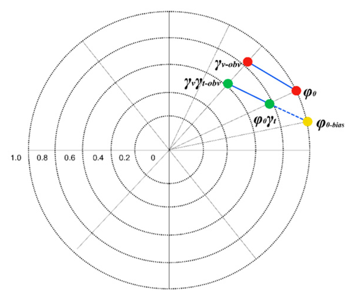
The distribution of the volume coherence (γv-obv) and the ground phase (φ0) in the unit circle are indicated by red dots in Figure 1 when there is no temporal decorrelation. Considering the effects of temporal decorrelation, volume coherence is more severely affected by this issue, especially in the case of low forests. With an increase in the temporal decorrelation factor of volume scattering (γTV), the volume coherence (γv-obv) shifts to γvγt-obv in the direction of the center of the unit circle [20,21], causing the ground phase estimated by the RVoG model also to shift (yellow dots in Figure 2), at which point the ground phase calculated by the RVoG model is expressed by φ0-bias. Figure 2 shows that the volume and ground phases are misestimated as a result of the effects of temporal decorrelation, which leads to an increase in phase center height of the volume coherence and ultimately leading to an overestimation of the forest height.
2.4.2. Analysis of the Error Sources of Underestimation for Tall Canopy
The strong penetration of the L-band accurately reflects the vertical structure information of the forest. However, electromagnetic wave signal penetration causes the center of the complex coherence phase to shift downward, resulting in an underestimation of the forest canopy height [10,31]. As shown in Figure 3, the penetrating character of SAR data causes the observed value of the volume coherence (γv-obv) to typically be situated below the top of the canopy. In contrast, the true phase center of the top of the forest canopy should be γv-dep. This effect causes the height of the volume phase center to be anomalously low, resulting in an underestimation of the forest height. When the forest is low, the effect of temporal decorrelation is increased, and the volume coherence becomes γvγt-obv. Owing to the penetration of SAR data, the true volume coherence phase center should be γvγt-dep; however, further assessment is required to determine whether underestimation or overestimation is dominant in this case.
2.5. Error Correction of the RVoG Model Based on Penetration Depth
2.5.1. Method of Underestimation Correction for Tall Canopy Height
Temporal decorrelation in the RVoG model often leads to overestimation of low vegetation; in taller vegetation areas, despite the relatively minimal influence of temporal decorrelation, the penetration depth of SAR becomes the main source of error. This issue is especially prominent in the L band, for which deeper penetration often results in underestimation of forest height, a problem that has been consistently difficult to resolve. To date, no relevant studies have been conducted to explore this issue; accordingly, in this work, we used penetration depth to correct RVoG model errors to counteract underestimation and overestimation in the RVoG model.
In taller vegetation areas, penetration depth is the main source of error and can be used to correct for the resulting underestimation. Equation (6) is the correction formula for underestimation, where HRVoG is the canopy height estimated by the RVoG model, Hd is the penetration depth, and HRVoG−cor is the corrected forest canopy height.
In a study on InSAR penetration depth estimation, Dall [31] proposed the only theoretical framework for estimating the penetration depth of infinitely deep volumes, which is a highly useful approach for directly calculating the penetration depth of SAR data. This theory proposes that the height deviation (Hd) can be calculated according to the phase-normalized interferometric phase (∠γ) and the vertical wave number (kz), as shown in Equation (7).
where kz is the vertical wave number. Another important interference parameter is the height of ambiguity (HoA), which represents the height difference between the two interferometric phase differences [10,31].
where HoA represents the ambiguous height in the air. Considering volume refraction, HoA can be expressed as:
where n is the refractive index. The complex coherence in an infinitely deep volume can be expressed as:
where d2 is a measure of the two-way penetration depth. According to Dall [31], d2/HoAVol correlates with the coherence amplitude, and the normalized interference phase (∠γ) can be derived from Equation (10):
In our study, the refraction (n) in the volume was assumed to be negligible. Thus, the height of ambiguity in the air was used to calculate the penetration depth.
The above condition applies to infinitely deep volumes; Dall [31] showed that when the ratio of canopy height to penetration depth (CH/Hd) is greater than 2–5, the forest can be considered as an infinitely deep volume. In this study, we denoted this ratio as P; if the infinity condition is not met, i.e., P is less than 2, then the analysis may be biased.
2.5.2. Method of Overestimation Correction for Low Canopy Height
There are two sources of error when the forest is low; the first is overestimation caused by temporal decorrelation, and the second is underestimation caused by penetration. These effects appear to cancel out; however, when the overestimation resulting from temporal decorrelation is greater than or equal to the penetration depth error, the overestimation can be compensated for by subtracting the penetration.
2.5.3. Simulation Experiments
To illustrate the relationship between forest canopy height and penetration depth in the RVoG model inversion, assume that in a scene, the corresponding incidence angle is Inc = 0.30 rad, the vertical effective wave number is kz = 0.12, the ground phase is φ0 = 0 rad, the extinction coefficient us σ = 0.0001, and the phase center height of the volume coherence is hv = 15 m. According to RVoG model Equation (2), the volume coherence is γv-obv = 0.87+0.29i, and the penetration depth is Hd = 4.40 m according to Equation (11), corresponding to a real forest height of Hcor = 19.40 m according to Equation (6).
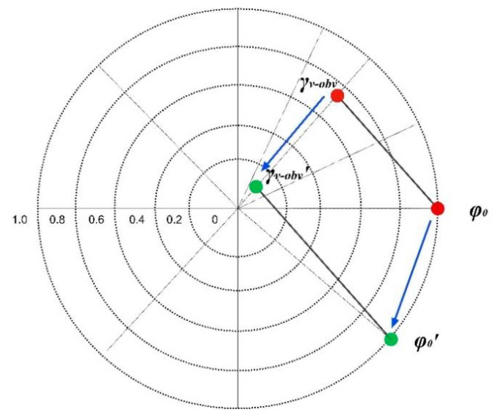
To simulate the variation law of forest height estimation error, variations in penetration depth caused by changes in volume coherence and ground phase under various temporal decorrelation conditions can be considered. Based on the above conditions, we assumed that the volume coherence (γv-obv) changes from γv-obv to γv-obv’ and that the ground phase gradually changes from φ0 to φ0′ as a result of temporal decorrelation, as shown in Figure 4. The following RVoG model and penetration depth model were used to calculate the forest height error (Equation (14)) and penetration depth variation caused by the abovementioned variation processes, as shown in Figure 5a. We simulated the variation law of the infinite-depth volume condition P (Equation (15)) under different conditions, as shown in Figure 5b.
The simulation results illustrate that when the temporal decorrelation effect is small, the height predicted by the RVoG model is lower than the true forest height (Figure 5a), and the underestimation error is approximately equal to the penetration depth; in this scenario, the penetration depth can be used to correct for underestimation. However, as the effect of temporal decorrelation gradually increases, the forest height error gradually changes from underestimation to overestimation. When the overestimated error value is greater than or equal to the penetration depth, the overestimation error can be corrected by the penetration depth. Secondly, as shown by the variation pattern of p-values (Figure 5b), when the decorrelation effect is small, p-values are greater than 3 (consistent with the infinitely deep volume scenario), and the forest height is underestimated—a finding that is consistent with the theoretical hypothesis of Dall [31]. Our results also indicate that when the forest height is overestimated, P is less than 3. The errors of underestimation and overestimation relative to penetration depth are shown schematically in Figure 6.
2.6. Determination of Correction Thresholds
The material above describes how to correct the underestimation of tall canopy and overestimation of low canopy in RVoG model inversion results using penetration depth; however, identification of overestimation or underestimation is key to the height correction step. Here, we propose two schemes to determine the threshold value of the correction interval.
2.6.1. Correction Threshold Determination Based on Reference Height (RH100)
The results reported by Lee [19,20,21,22,23] show that temporal decorrelation has a greater effect on low forests, whereas forest height estimation errors in tall vegetation areas (i.e., infinitely deep volumes) are mainly underestimated, owing to the effect of microwave penetration [31]. We propose correcting for these two errors using the penetration depth; however, both underestimation and overestimation correction of forest height require a specific threshold to determine the correction interval. Accordingly, in this study, we used LiDAR canopy height (RH100) as a reference to determine the correction threshold using an iterative approach. For underestimation correction of tall forests, the threshold was set at 2 m intervals, and the correction result was calculated once for each height threshold value, i.e., the RVoG model inversion height plus the penetration depth, where RH100 is greater than the height threshold. For instances, where RH100 is less than the height threshold, the RVoG model inversion result remains unchanged. Each iteration returns a set of R2 and RMSE values between the corrected RVoG model inversion height and RH100. The method of determining the correction threshold for low forest overestimation the same as that described above; the penetration depth is subtracted from the RVoG model inversion height when RH100 is below the height threshold, the RVoG model inversion result is unchanged when RH100 is greater than the height threshold, and the coefficient of determination (R2) and root mean square error (RMSE) values are calculated between the inversion height and RH100 after each correction. Two threshold values (Hh and Hl) are thus obtained.
2.6.2. Correction Threshold Determination Based on p-Value
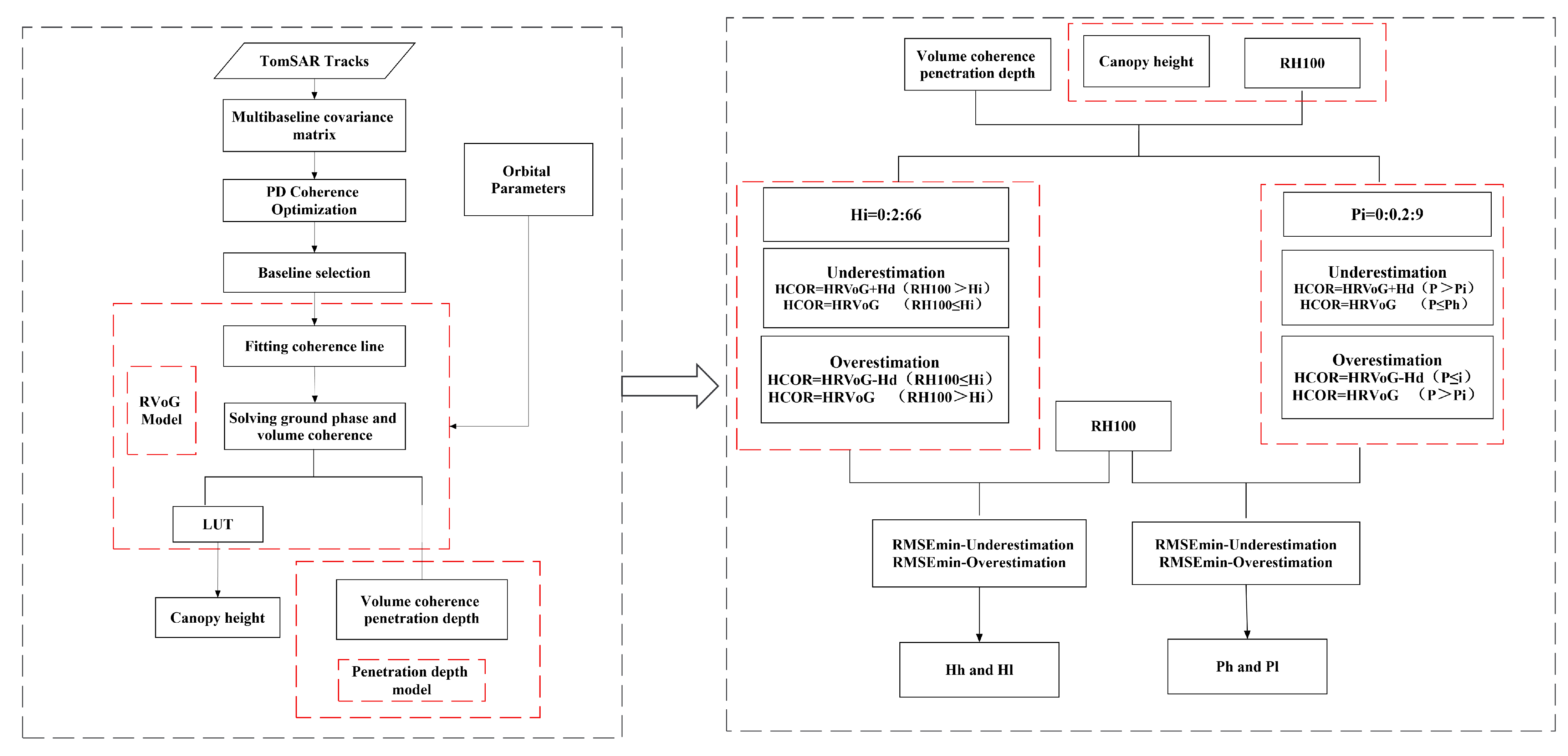
Dall [31] showed that the height bias of InSAR/PolInSAR in an infinitely deep volume (p > 2–5) can be corrected by the penetration depth. This finding was verified in our simulation experiments. However, another conclusion drawn from the simulation experiments in this study is that when p < 3, the forest height is underestimated; in addition, overestimation error can be mitigated using penetration depth. This conclusion provides an important basis for determining forest height underestimation and overestimation. In this scheme, the p-value is used as a reference to iteratively determine the correction threshold for underestimation and overestimation. For underestimation correction of higher forests, the threshold value was set at 0.2 intervals, and each threshold value was corrected once, i.e., when P is greater than the height threshold, the penetration depth is added to the RVoG model inversion height, and when P is less than the height threshold, the RVoG model inversion results remain unchanged; each iteration returns a set of R2 and RMSE between the corrected RVoG model inversion height and RH100. The method of determining the correction threshold for overestimation is analogous. When P is less than the height threshold, the penetration depth is subtracted from the RVoG model inversion height; when P is greater than the height threshold, the RVoG model inversion result is unchanged; and the R2 and RMSE values between the corrected inversion height and RH100 are calculated. Two threshold values (Ph and Pl) are thus obtained. The workflow of this study is shown in Figure 7.
2.7. Model Evaluation Indicators
The model results were evaluated using the R2, RMSE, and bias (BIAS) indicators.
where Hi is the LiDAR canopy height, i is the mean canopy height according to PolInSAR, and i is the PolInSAR inversion canopy height value.
3. Results
We selected 6357 samples in the Lope test area and divided them into training and test sample datasets (train = 4239, test = 2118). Pongara test area had 4602 samples (train = 3068, test = 1534). The training samples were used to iteratively determine the correction threshold and fit the machine learning model. The validation samples were used to verify the corrected thresholds and the machine learning model.
3.1. Error Correction Based on Reference Height (RH100)
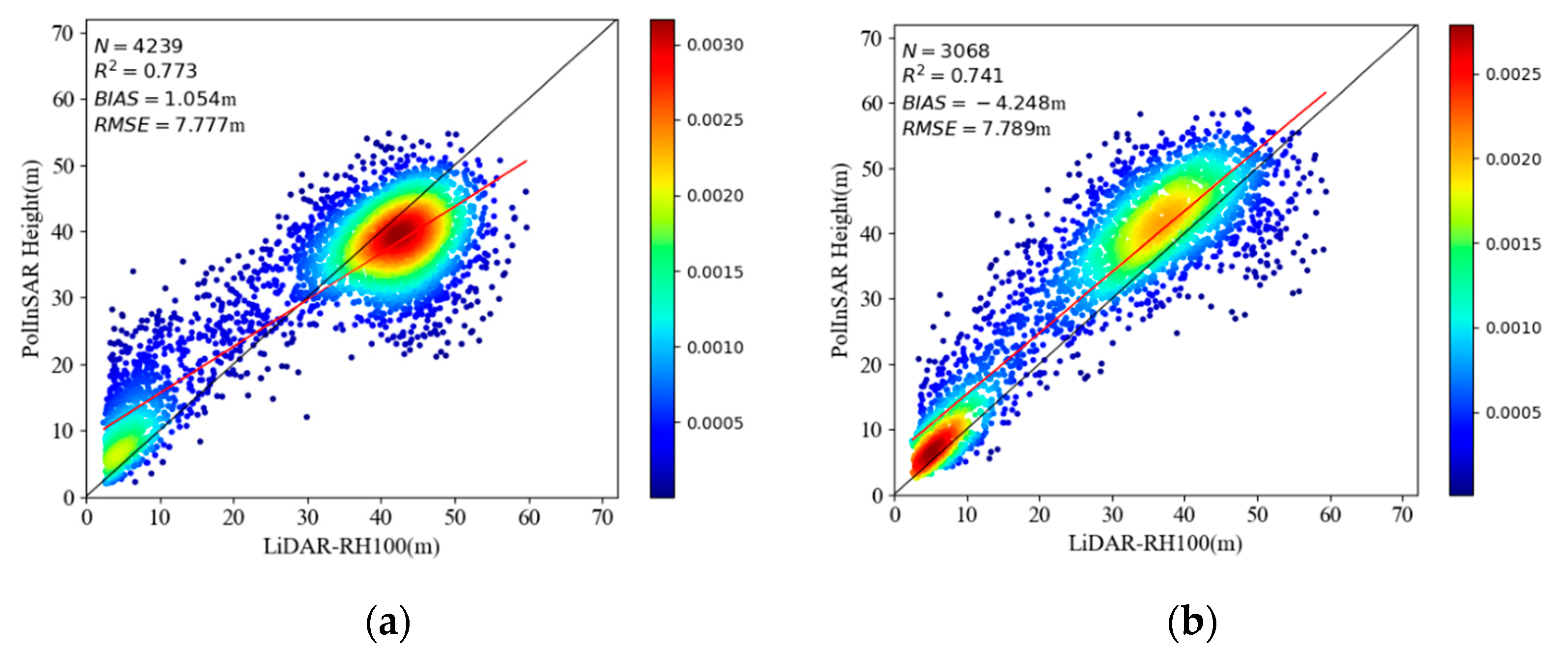
The inversion results from the RVoG model show that both underestimation of tall canopy and overestimation of low canopy occurred in the Lope and Pongara experimental areas. The underestimation of tall canopy areas is pronounced in the Lope experimental area when the forest height exceeds 40 m, and low canopy overestimation is prominent when the forest height is less than 30 m. The Pongara test area is associated with a more obvious overestimation of low canopy areas and a relatively minimal underestimation of tall canopy. This result is consistent with our previous theoretical hypothesis that overestimation is more severely affected by temporal decorrelation in low vegetation areas and that SAR penetration causes underestimation in tall vegetation areas (Figure 8). Accordingly, the LiDAR-derived reference height (RH100) was used to determine the correction thresholds for underestimation and overestimation.
The iterative results for the correction thresholds for the Lope test area are shown in Table 3. To correct tall canopy underestimation, when the height threshold exceeds 42 m, the accuracy of the corrected value is higher than that before the correction, with the highest accuracy achieved at a height threshold of 46 m, corresponding to an R2 value of 0.817 and an RMSE of 6.995 m. The low canopy overestimation was improved when the height threshold was in the range of 4–38 m, with the best results achieved for a height threshold of 30 m, corresponding to an R2 value of 0.813 and an RMSE of 7.056 m.
In the Pongara test area, when correcting for underestimation of tall canopy, the results were improved when the height threshold was greater than 50 m. The R2 values of the corrected results were all higher than those of the precorrection results, and the RMSE values were all lower than those of the precorrection results; however, the differences were marginal because the underestimation of tall canopy was relatively less pronounced in this study area. The highest accuracy was achieved when the height threshold was set at 54 m, corresponding to an R2 value of 0.744 and an RMSE of 7.743 m. When correcting for low canopy overestimation, when the height threshold was in the range of 8–46 m, the accuracy of the results improved; the highest accuracy was achieved for a height threshold of 34 m, with an R2 value of 0.854 and an RMSE of 5.839.
After determining the thresholds for various correction schemes, independent samples were used to validate the thresholds. The results of this analysis show that the R2 value increased from 0.775 to 0.814, and the RMSE decreased from 7.748 m to 7.031 m in the Lope test area after correcting for low canopy overestimation with RH100 < 30 m as the threshold (Figure 9b), with a significant improvement in low-value overestimation exhibited by the scatter plot. After tall canopy correction with RH100 > 46 m to correct for underestimation (Figure 9c), the R2 value increased from 0.775 to 0.816, and the RMSE decreased from 7.748 m to 7.005 m. The best results were achieved with simultaneous correction of overestimation and underestimation (i.e., RH100 < 30 m and RH100 > 42 m; Figure 9c). In this scenario, the R2 value increased from 0.775 to 0.856, and the RMSE decreased from 7.748 m to 6.204 m, with significant improvements in both underestimation and overestimation (Figure 9d). In the Pongara test area, correction for overestimation of low canopy with RH100 < 34 m (Figure 9f) led to an increase in R2 from 0.752 to 0.850 and a decrease in RMSE from 7.628 m to 5.931 m, with a significant improvement in low canopy overestimation exhibited in the scatter plot. Similarly, for tall canopy underestimation correction with RH100 > 54 m (Figure 9g), the R2 value increased from 0.752 to 0.755, and the RMSE decreased from 7.628 m to 7.570 m. The best results were achieved when correcting for both overestimation and underestimation (i.e., RH100 < 34 m and RH100 > 54 m; Figure 9f), with R2 increasing from 0.752 to 0.854 and RMSE decreasing from 7.628 m to 5.856 m, with significant improvements in terms of both underestimation and overestimation (Figure 9h). The results for both study areas demonstrate that it is effective to use the true forest height as a reference height threshold to correct inversion bias in the RVoG model; however, the scatter plots show that some samples were overcorrected in both study areas. The key limitation of this RVoG inversion bias correction method is its requirement of a true height reference; thus, the extrapolation scalability of this method is limited. Furthermore, the optimum correction thresholds for the two study areas differ, likely primarily owing to varying temporal decorrelation of SAR data, spatial baseline size, and inconsistent forest structure in the two experimental areas.
3.2. Error Correction Based on the p-Value
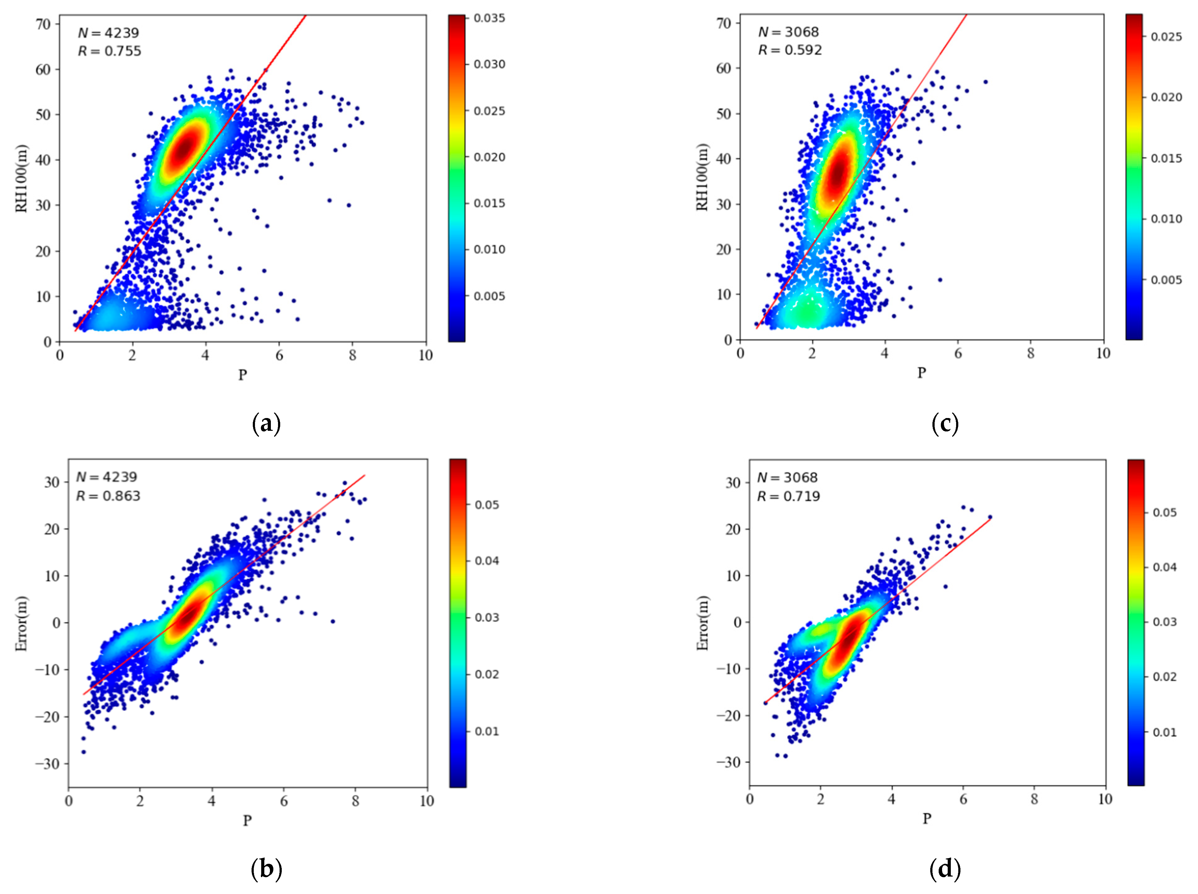
Previous theoretical models and experimental simulations suggest that the penetration depth is approximately equal to the underestimation error when the infinite-depth volume determination condition (P) is greater than 3, which is consistent with the conclusion of Dall’s [31] study. In addition, our experimental results suggest that when P is less than 3, the overestimation error can be improved using the penetration depth. The scatter plot of the error distribution also shows that in the Lope experimental area (Figure 10b), the correlation coefficient (R) between the p-value and the RVoG model inversion error is 0.863. With increasing p-value, the error gradually changes from negative to positive, with increased underestimation of tall canopy samples. This observation is consistent with the performance pattern shown in Figure 9a, as the forest height distribution in the Lope experimental area shows a polarization phenomenon, i.e., tall and low vegetation types are more common, whereas medium-height vegetation types are less abundant. The correlation coefficient between the p-value and inversion error was 0.719 in the Pongara test area, and the error gradually changed from negative to positive with increasing p-value. This observation is consistent with the results in the Lope test area. However, the overestimation of the low canopy was more obvious in the Pongara test area, as shown in Figure 10d. There was more low vegetation in the Pongara test area. In addition, based on the variation patterns of the p-value, the linearity pattern of both experimental areas was improved when the p-value was greater than 3. Such a pattern is also consistent with our previous experimental hypothesis that when the p-value exceeds 3, the infinite-depth volume condition is valid; in this case, the penetration depth is the main source of error. When the p-value is less than 3, both temporal decorrelation and penetration error occur.
As the p-value is a reliable indicator of both overestimation and underestimation, the corresponding correction thresholds are determined by the p-value. The data from the Lope test area show that the results for the correction of tall canopy underestimation are improved relative to the precorrection results when P is in the range of 3.6–8.0. The highest accuracy was obtained when P was 3.8, corresponding to an R2 value of 0.865 and an RMSE of 5.996 m. In the low canopy overestimation correction results, when P was in the interval of 0.6–3, the corrected results were all improved relative to the precorrection results. The highest accuracy was achieved with a p-value of 2.6, corresponding to an R2 value of 0.823 and an RMSE of 6.877 m (see Table 4).
In the Pongara test area, the corrected results for underestimation of the tall canopy were improved relative to the precorrection results when P was in the interval of 3.6–4.4. The best results were obtained for tall canopy underestimation correction with a p-value of 3.8, corresponding to an R2 value of 0.758 and an RMSE of 7.531 m. In the corrected results for low canopy overestimation, the corrected results were improved relative to the precorrection results when P was in the interval of 1.2–3.2; in this scenario, a p-value of 2.4 corresponded to the highest accuracy, with an R2 value of 0.880 and an RMSE of 5.308 m.
After the correction thresholds for the various compensation schemes were determined in the previous step, independent samples were used to validate the results after correction for the thresholds. The results for the Lope test area show that the R2 value increased from 0.775 to 0.824, and the RMSE decreased from 7.748 m to 6.851 m after correcting for overestimation of the low canopy at p < 2.6, with a significant improvement in low canopy overestimation reflected by the corresponding scatter plot (Figure 11a). When correcting for tall canopy underestimation for p > 3.8 (Figure 11b), the R2 value increased from 0.775 to 0.865, and the RMSE decreased from 7.748 m to 6.004 m, with a similar significant improvement reflected by the tall canopy underestimation in the scatter plot. The best results were obtained by correcting for both factors with thresholds of p < 2.6 and p > 3.8 (Figure 11c), with the R2 value increasing from 0.775 to 0.914 and RMSE decreasing from 7.748 m to 4.796 m; in addition, significant improvements in both underestimation and overestimation were achieved, as shown in the scatter plot. In the Pongara test area, the accuracy improved significantly when correcting for low canopy overestimation at p < 2.4 (Figure 11d), with the R2 value increasing from 0.752 to 0.877 and the RMSE decreasing from 7.628 m to 5.357 m. A significant improvement in the overestimation of the low canopy is illustrated in the scatter plot. At p > 3.8, when correcting for tall canopy underestimation (Figure 11e), the R2 value increased from 0.752 to 0.770, and the RMSE decreased from 7.628 m to 7.340 m. The highest accuracy was achieved when a correction for p < 2.4 and p > 3.8 (Figure 11f) was applied; in this case, the R2 value increased from 0.752 to 0.896, and the RMSE decreased from 7.628 m to 4.939 m, with both underestimation and overestimation significantly improved.
The results of our study demonstrate that the p-value can be effectively used as a threshold to correct the inversion error of the RVoG model. The corrected results are markedly different from the original inversion results, and the results achieved using the p-value as the correction threshold are significantly better than those obtained using the reference height as the correction threshold. Results from the test and validation samples show the same pattern, with relatively few overcorrected samples and increased overall accuracy under p-value correction. However, there are still a few sample points that are uncorrected for errors, as noted above; the decorrelation, ground-to-volume magnitude ratio, baseline, and vegetation conditions may influence this aspect.
3.3. p-Value Prediction Based on Machine Learning
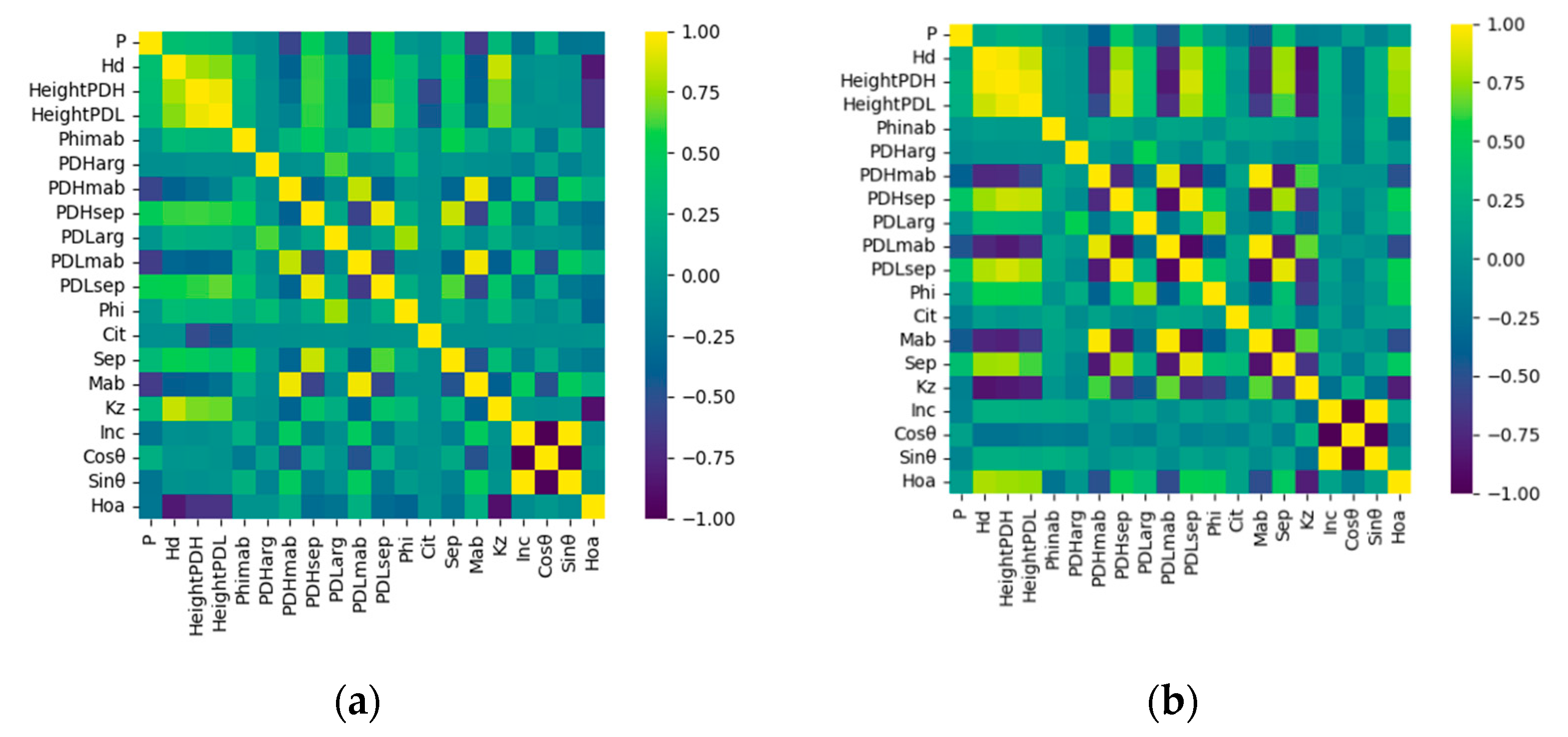
According to the above results, using the p-value as the correction threshold to improve the RVoG model’s inversion error yields improved results. However, calculating P typically requires the true forest canopy height as an input, which is not suitable as a solution at large, regional scales. Therefore, we propose a machine learning approach to invert p-values, allowing valid p-values to be obtained without actual tree height measurements; on this basis, error correction of the forest canopy height estimated by the RVoG model can be achieved. The p-value inversion was performed as follows. RH100 was used as the training sample, and parameters derived from the RVoG three-stage method, i.e., penetration depth, polarization interference information, and orbit information, were used as independent variables (Table 5, Figure 12). A random forest regression model [40,41,42] was used to invert p values.
To ensure consistency with the sample data in reported in the above sections, 4239 and 3068 samples were used model training in the Lope and Pongara regions, respectively; the scatter of the independent validation samples is shown in Figure 13. During construction of the random forest model, the model parameters were optimized twice, first using a random iterative method to obtain the local optimal parameters, followed by a grid-search function to determine the global optimal parameters, thus avoiding model overfitting or underfitting. In the Lope test area, the R2 of the model validation result was 0.732, and the RMSE was 0.593; in the Pongara test area, the R2 of the validation result was 0.568, and the RMSE was 0.486. Despite some differences between the inversion results of the two test areas, our analysis suggests that this mainly arose as a result of differences in forest height between the two study areas, decorrelation of the SAR data, the baseline size, and other uncertainties. In the following sections, the p-value from the random forest model inversion is used as a threshold to correct the inversion error of the RVoG model.
3.4. Error Correction Based on PRF
The threshold value determined above was combined with the machine learning-predicted p-value (PRF) in this scheme to correct the RVoG model error. In the Lope test area, the inversion accuracy after correcting for low canopy overestimation when PRF < 2.6 was improved relative to the initial RVoG model inversion results (Figure 14a,b). The R2 value increased from 0.775 to 0.801, the RMSE decreased from 7.748 m to 7.283 m, and low canopy overestimation was partially corrected, as shown in the scatter plot. Some improvement was also achieved when PRF > 3.8 (Figure 14c); using the penetration depth correction for tall canopy underestimation correction, the R2 value increased from 0.775 to 0.819, the RMSE decreased from 7.748 m to 6.945 m, and the scatter plot demonstrates that tall canopy underestimation was corrected to some extent. Overall, the highest inversion accuracy was obtained when PRF < 2.6 and PRF > 3.8 were corrected (Figure 14d); in this case, the R2 value was 0.845, and the RMSE was 6.422 m, with both underestimation and overestimation corrected to some extent. In the Pongara test area, the accuracy of the inversion corrected for low canopy overestimation at PRF < 2.4 was also improved relative to that of the initial inversion result of the RVoG model (Figure 14e,f), with the R2 value increasing from 0.752 to 0.770, the RMSE decreasing from 7.628 m to 7.337 m, and low canopy overestimation corrected to some extent. Similarly, the accuracy of the inversion corrected for tall canopy underestimation at PRF > 3.8 was improved relative to that of the inversion result of the RVoG model (Figure 14g). The R2 increased from 0.752 to 0.761, and the RMSE decreased from 7.628 m to 7.481 m, with tall canopy underestimation corrected to some extent, as shown in the scatter plot. The highest inversion accuracy was recorded when correcting for both PRF < 2.4 and PRF > 3.8 (Figure 14h), with an R2 value of 0.780 and an RMSE of 7.184 m, with partial correction of both underestimation and overestimation achieved. Therefore, we predicted the p-value of the whole experimental area using the random forest model and corrected the forest canopy height of the whole study area based on PRF, as shown in Figure 15.
The patterns in these results are consistent with those in the results reported in the previous section, indicating that the use of a machine learning approach to invert the p-value as a correction threshold is an effective method to improve the accuracy of the inversion results of the RVoG model. The results for the Lope test area were improved significantly, whereas the results for the Pongara test area improved but to a lesser extent, primarily owing to the precision of the p-value; an error in the p-value predicted by the machine learning method leads to overcorrection or undercorrection. This scenario is most obvious in the Pongara test area, owing to the relatively large error in p-values in this test area.
4. Discussion
The RVoG model is the most effective forest height inversion model. However, it is susceptible to the dual problems of tall canopy underestimation and low canopy overestimation. L-band SAR data have strong penetration and can fully reflect the forest height information in tropical rainforests. However, this strong penetration can lead to forest canopy height estimation errors. Simard and Denbina [43] proposed the RMoG model to correct forest height estimation error caused by temporal decorrelation. Other researchers have used the RVoG-VDT model to mitigate the temporal decorrelation effect [44]. However, this approach has complex solution processes. The method proposed in this paper is not affected by the abovementioned conditions and improves tall canopy underestimation and low canopy overestimation significantly in the RVoG model inversion results, with improved inversion accuracy (see Table 6).
In this study, we used the RH100 LiDAR relative height variable of as a reference value to correct for the forest canopy height estimation error; despite some error between RH100 and the real forest canopy height, this error does not affect our experimental conclusions. LiDAR can obtain high-precision forest vertical structure parameters, especially forest height, whereas PolInSAR is based on microwave scattering theory to estimate forest height, which is affected by wavelength penetration and temporal decorrelation, with increased uncertainties; therefore, additional samples are needed to illustrate the variation pattern in the validation of the results. LiDAR is currently the most effective way to replace manual ground-based forest canopy height measurements to validate and calibrate PolInSAR forest canopy height estimates so that the results are closer to the LiDAR canopy heights and closer to the true values. Accordingly, this has become a common way to verify the results of PolInSAR forest canopy height estimation based on LiDAR canopy height [10,11,16,35,45].
In the reference height-based correction results, there is clear overcorrection and undercorrection. The reasons for this are twofold. First, the height thresholds are determined by iteration’ these thresholds are only empirical, and their values differ considerably between the two test areas, with height correction thresholds of 30 m and 46 m in the Lope test area and 34 m and 54 m in the Pongara test area. The scatter plots also reveal that not all samples overestimate in low vegetation areas and not all samples underestimate in tall vegetation areas. This variability may be related to factors such as the depression of the forest, the ground-to-volume magnitude ratio, and the imaging geometry parameters. We corrected the RVoG model inversion results using a fixed threshold, which can reduce the overall error. However, this approach also inevitably caused overcorrection and undercorrection in some samples. From a theoretical perspective, tall canopy underestimation is mainly caused by penetration. Furthermore, under practical conditions, the error magnitude is not exactly equal to the penetration depth, owing to the contribution of other factors. For low vegetation, when the overestimation caused by temporal decorrelation is much larger or smaller than the penetration depth, error correction using the penetration depth results in overcorrection or undercorrection.
The results achieved using p-value correction are better than those obtained using the reference height, and the thresholds determined by this method are more stable. The correction thresholds were 2.6 and 3.8 for the p-value in the Lope test area, and 2.4 and 3.8 in the Pongara test area, illustrating improved consistency between the two test areas. This result is consistent with our simulation experiments. However, it is still impossible to avoid overcorrection and undercorrection using the p-value as the correction threshold for the reasons described above. Penetration is the main error source in infinitely deep volumes, and the penetration depth in this case is closer to the inverse error of the RVoG model. Using P as the correction threshold is consistent with the infinitely deep volume condition; thus, the tall canopy underestimation correction results are improved. In contrast, when the p-value is small, although low canopy overestimation still occurs, using the penetration depth as a correction can only reduce the overestimation error to some extent; in this scenario, the error does not exactly match the size of the penetration depth. The results of our simulation experiments show that the overestimation error increased with the gradual increase in the temporal decorrelation effect. Under actual forest conditions, the temporal decorrelation also varies as a result of differences in forest structure and baseline combinations. When the overestimation caused by temporal decorrelation is considerably larger than the penetration depth value, the error can be reduced by subtracting the penetration depth. However, when the overestimation of temporal decorrelation is smaller than the penetration depth, the error cannot be reduced by the penetration depth, and overcorrection and undercorrection occur. This difference is also related to the number of baselines, and the temporal decorrelation is inconsistent under different baseline combinations. In the future, research cases can be tested to prove whether p-values achieve satisfactory generalization performance as correction thresholds.
We used a machine learning approach in the last experimental scheme to predict global p-values from local LiDAR canopy height data combined with polarized interferometric feature variables. This approach was then used to correct the RVoG model canopy height using the penetration depth, thus achieving global-scale forest canopy height discrimination and correction of underestimation and overestimation. However, there are errors in the p-values predicted by machine learning, resulting in overcorrection or undercorrection of the results; thus, other p-value determination methods could be explored in future studies.
Another factor that affected the correction results was the baseline selection method. Related studies [43] have identified that when relying purely on the distribution law of complex coherence to select baselines, the final baseline combinations do not necessarily match the actual forest conditions. Moreover, the temporal decorrelation between baseline combinations is inconsistent and notably more significant in low vegetation areas, generating sources of error. Thus, Denbina et al. [43] improved underestimation and overestimation by optimizing baseline selection through machine learning methods; our proposed method achieves the same purpose with increased accuracy, and the underlying theory is equally applicable to single baselines, which can be further explored in future research.
5. Conclusions
Temporal decorrelation and penetration are two important factors that lead to underestimation and overestimation in forest canopy height inversion using the RVoG model. In this study, we used the penetration depth to correct the forest canopy height inversion results of the RVoG model. We conclude that (1) the true forest height can be used to constrain the underestimation and overestimation range of the RVoG model inversion results, and the underestimation and overestimation of the RVoG model inversion result can be corrected using the penetration depth. This approach can effectively correct the underestimation error in tall forests caused by penetration and reduce the overestimation error caused by temporal decorrelation in low forests. (2) The p-value of the infinite-depth volume criterion is more accurate in determining the underestimation and overestimation of the RVoG model inversion results compared to the true forest height-based correction method. Our results show that p > 3 indicates underestimation in the RVoG model inversion results, and p < 3 indicates overestimation. Using the p-value as a threshold to correct the inversion results of the RVoG model results in improved estimation accuracy. (3) The global-scale p-value can be predicted using machine learning methods combined with polarized interference features. In addition, it is effective to use p-values predicted by machine learning methods as a threshold to correct the error of the inversion results of the RVoG model, with improved accuracy achieved after correction. As the RVoG model is the most widely used forest height inversion model, it is necessary to improve the accuracy of forest height inversion by improving the model error in a targeted way. GEDI and ICESat-2 have acquired a large amount of laser point data. With the application of ALOS-2 and SAOCOM satellite data, as well as the recently realized TanDEM-L and BIOMASS satellites and the NISAR program, the approach presented in this paper will have important implications for accurate estimation of forest height in future research.
Author Contributions
H.L. designed the experiments, completed the data analysis, and wrote the paper; C.Y. provided important guidance for experimental design, data analysis, and writing of the paper; N.W. assisted with the experiments; G.L. assisted with data processing; and S.C. assisted with the development of graphs. All authors have read and agreed to the published version of the manuscript.
Funding
This research was funded by the National Natural Science Foundation of China “Multi-frequency SAR polarized interferometric data for forest tree height inversion” (Grant No. 42061072); the Major Science and Technology Special Project of Yunnan Provincial Science and Technology Department “Forest Resources Digital Development and Application in Yunnan” (Grant No. 202002AA100007-015); and the Scientific Research Fund Project of Yunnan Provincial Education Department “Forest height inversion from starborne microwave data TanDEM-X combined with topographic data” (Grant No. 2022Y579).
Data Availability Statement
UAVSAR data and LiDAR-RH100 were obtained from NASA’s Oak Ridge National Laboratory Biogeochemical Dynamics Distributed Active Archive Center (https://daac.ornl.gov/cgi-bin/dataset_lister.pl?p=38 (accessed on 19 October 2021)) and Jet Propulsion Laboratory (https://uavsar.jpl.nasa.gov (accessed on 24 December 2021)).
Acknowledgments
Thanks to NASA for providing all the publicly available free datasets to support this work.
Conflicts of Interest
No conflict of interest exists in association with the submission of this manuscript, and the manuscript has been approved for publication by all authors.
References
- Izzawati, I.H.W.; Wallington, E.D.; Woodhouse, I.H. Forest height retrieval from commercial X-band SAR products. IEEE Trans. Geosci. Remote Sens. 2006, 44, 863–870. [Google Scholar] [CrossRef]
- Laurin, G.V.; Ding, J.; Disney, M.; Bartholomeus, H.; Valentini, R. Tree height in tropical forest as measured by different ground, proximal, and remote sensing instruments, and impacts on above ground biomass estimates. Int. J. Appl. Earth Obs. Geoinf. 2019, 82, 101899. [Google Scholar]
- Chen, W.; Zhao, J.; Cao, C.X.; Tian, H.J. Shrub biomass estimation in semi-arid sandland ecosystem based on remote sensing technology. Glob. Ecol. Conserv. 2018, 16, e00479. [Google Scholar]
- Ghulam, A.; Porton, I.; Freeman, K. Detecting subcanopy invasive plant species in tropical rainforest by integrating optical and microwave (InSAR/PolInSAR) remote sensing data, and a decision tree algorithm. ISPRS J. Photogramm. Remote Sens. 2014, 88, 174–192. [Google Scholar] [CrossRef]
- Chen, W.; Zheng, Q.; Xiang, H.; Chen, X.; Sakai, T. Forest Canopy Height Estimation Using Polarimetric Interferometric Synthetic Aperture Radar (PolInSAR) Technology Based on Full-Polarized ALOS/PALSAR Data. Remote Sens. 2021, 13, 174. [Google Scholar] [CrossRef]
- Zhang, L.; Duan, B.; Zou, B. Research on Inversion Models for Forest Height Estimation Using Polarimetric SAR Interferometry. Int. Arch. Photogramm. Remote Sens. Spat. Inf. Sci. 2017, 42, 659–663. [Google Scholar] [CrossRef] [Green Version]
- Garestier, F.; Le Toan, T. Forest modeling for height inversion using single-baseline InSAR/Pol-InSAR data. IEEE Trans. Geosci. Remote Sens. 2009, 48, 1528–1539. [Google Scholar]
- Kumar, S.; Govil, H.; Srivastava, P.K.; Thakur, P.K.; Kushwaha, S.P. Spaceborne multifrequency PolInSAR-based inversion modelling for forest height retrieval. Remote Sens. 2020, 12, 4042. [Google Scholar] [CrossRef]
- Wang, C.; Wang, L.; Fu, H.; Xie, Q.; Zhu, J. The impact of forest density on forest height inversion modeling from polarimetric InSAR data. Remote Sens. 2019, 8, 291. [Google Scholar] [CrossRef] [Green Version]
- Schlund, M.; Baron, D.; Magdon, P.; Erasmi, S. Canopy penetration depth estimation with TanDEM-X and its compensation in temperate forests. ISPRS J. Photogramm. Remote Sens. 2019, 147, 232–241. [Google Scholar] [CrossRef]
- Qi, W.; Lee, S.K.; Hancock, S.; Luthcke, S.; Tang, H.; Armston, J.; Dubayah, R. Improved forest height estimation by fusion of simulated GEDI Lidar data and TanDEM-X InSAR data. Remote Sens. Environ. 2019, 221, 621–634. [Google Scholar] [CrossRef] [Green Version]
- Hajnsek, I.; Kugler, F.; Lee, S.K. Tropical-forest-parameter estimation by means of Pol-InSAR: The INDREX-II campaign. IEEE Trans. Geosci. Remote Sens. 2009, 47, 481–493. [Google Scholar]
- Praks, J.; Kugler, F.; Papathanassiou, K.P.; Hajnsek, I.; Hallikainen, M. Height estimation of boreal forest: Interferometric model-based inversion at L-and X-band versus HUTSCAT profiling scatterometer. IEEE Geosci. Remote Sens. 2007, 4, 466–470. [Google Scholar] [CrossRef]
- Liao, Z.; He, B.; Quan, X.; van Dijk, A.I.; Qiu, S.; Yin, C. Biomass estimation in dense tropical forest using multiple information from single-baseline P-band PolInSAR data. Remote Sens. Environ. 2018, 221, 489–507. [Google Scholar]
- Treuhaft, R.N.; Moghaddam, M.; van Zyl, J.J. Vegetation characteristics and underlying topography from interferometric radar. Radio Sci. 1996, 31, 1449–1485. [Google Scholar] [CrossRef]
- Liao, Z.; He, B.; van Dijk, A.I.; Bai, X.; Quan, X. The impacts of spatial baseline on forest canopy height model and digital terrain model retrieval using P-band PolInSAR data. Remote Sens. Environ. 2018, 210, 403–421. [Google Scholar] [CrossRef]
- Cloude, S.R.; Papathanassiou, K.P. Three-stage inversion process for polarimetric SAR interferometry. IEE Proc.-Radar Sonar Navig. 2003, 150, 125–134. [Google Scholar] [CrossRef] [Green Version]
- Mette, T.; Kugler, F.; Papathanassiou, K.; Hajnsek, I. Forest and the random volume over ground—Nature and effect of 3 possible error types. In Proceedings of the European Conference on Synthetic Aperture Radar (EUSAR), VDE Verlag GmbH, Dresden, Germany, 16–18 May 2006. [Google Scholar]
- Lee, S.-K.; Kugler, F.; Papathanassiou, K.P.; Hajnsek, I. Quantifying temporal decorrelation over boreal forest at L-and P-band. In Proceedings of the 7th European Conference on. VDE, Friedrichshafen, Germany, 2–5 June 2008. [Google Scholar]
- Lee, S.K.; Kugler, F.; Papathanassiou, K.; Moreira, A. Forest height estimation by means of Pol-InSAR limitations posed by temporal decorrelation. In Proceedings of the 11th ALOS Kyoto & Carbon Initiative, Tsukuba, Japan, 28 December 2009. [Google Scholar]
- Lee, S.K.; Kugler, F.; Hajnsek, I.; Papathanassiou, K. The impact of temporal decorrelation over forest terrain in polarimetric SAR interferometry. In Proceedings of the International Workshop on Applications of Polarimetry and Polarimetric Interferometry (Pol-InSAR). ESA, Frascati, Italy, 26–30 January 2009. [Google Scholar]
- Lee, S.K.; Kugler, F.; Papathanassiou, K.; Hajnsek, I. Multibaseline polarimetric SAR interferometry forest height inversion approaches. In Proceedings of the ESA POLinSAR Workshop, Frascati, Italy, 24–28 January 2011. [Google Scholar]
- Lee, S.K.; Kugler, F.; Papathanassiou, K.; Hajnsek, I. Quantification and compensation of temporal decorrelation effects in polarimetric SAR interferometry. In Proceedings of the 2012 IEEE International Geoscience and Remote Sensing Symposium, Munich, Germany, 22–27 July 2012. [Google Scholar]
- Solberg, S.; Astrup, R.; Weydahl, D.J. Detection of forest clear-cuts with shuttle radar topography mission (SRTM) and TanDEM-X InSAR data. Remote Sens. 2013, 5, 5449–5462. [Google Scholar] [CrossRef] [Green Version]
- Tanase, M.A.; Ismail, I.; Lowell, K.; Karyanto, O.; Santoro, M. Detecting and quantifying forest change: The potential of existing C- and X-band radar datasets. PLoS ONE 2015, 10, e0131079. [Google Scholar]
- Schlund, M.; von Poncet, F.; Hoekman, D.H.; Kuntz, S.; Schmullius, C. Importance of bistatic SAR features from TanDEM-X for forest mapping and monitoring. Remote Sens. Environ. 2014, 151, 16–26. [Google Scholar] [CrossRef]
- Weydahl, D.J.; Sagstuen, J.; Dick, O.B.; Ronning, H. SRTM DEM accuracy assessment over vegetated areas in Norway. Int. J. Remote Sens. 2007, 28, 3513–3527. [Google Scholar] [CrossRef]
- Treuhaft, R.; Goncalves, F.; dos Santos, J.; Keller, M.; Palace, M.; Madsen, S.; Sullivan, F.; Graca, P. Tropical-forest biomass estimation at X-band from the spaceborne TanDEM-X interferometer. IEEE Geosci. Remote Sens. Lett. 2015, 12, 239–243. [Google Scholar] [CrossRef] [Green Version]
- Kugler, F.; Schulze, D.; Hajnsek, I.; Pretzsch, H.; Papathanassiou, K. TanDEM-X Pol-InSAR performance for forest height estimation. IEEE Trans. Geosci. Remote Sens. 2014, 52, 6404–6422. [Google Scholar] [CrossRef]
- Varekamp, C.; Hoekman, D.H. High-resolution InSAR image simulation for forest canopies. IEEE Trans. Geosci. Remote Sens. 2002, 40, 1648–1655. [Google Scholar]
- Dall, J. InSAR elevation bias caused by penetration into uniform volumes. IEEE Trans. Geosci. Remote Sens. 2007, 45, 2319–2324. [Google Scholar] [CrossRef] [Green Version]
- Fore, A.G.; Chapman, B.D.; Hawkins, B.P.; Hensley, S.; Jones, C.E.; Michel, T.R.; Muellerschoen, R.J. UAVSAR polarimetric calibration. IEEE Trans. Geosci. Remote Sens. 2015, 53, 3481–3491. [Google Scholar] [CrossRef]
- Armston, J.; Tang, H.; Hancock, S.; Marselis, S.; Duncanson, L.; Kellner, J.; Hofton, M.; Blair, J.B.; Fatoyinbo, T.; Dubayah, R.O. AfriSAR: Gridded Forest Biomass and Canopy Metrics Derived from LVIS, Gabon, 2016; ORNL DAAC: Oak Ridge, TN, USA, 2020. [Google Scholar] [CrossRef]
- Papathanassiou, K.; Cloude, S.R. Single-baseline polarimetric SAR interferometry. IEEE Trans. Geosci. Remote Sens 2001, 39, 2352–2363. [Google Scholar] [CrossRef] [Green Version]
- Kugler, F.; Lee, S.K.; Hajnsek, I.; Papathanassiou, K.P. Forest height estimation by means of Pol-InSAR data inversion: The role of the vertical wavenumber. IEEE Trans. Geosci. Remote Sens. 2015, 53, 5294–5311. [Google Scholar] [CrossRef]
- Denbina, M.; Simard, M. Kapok: An open source Python library for PolInSAR forest height estimation using UAVSAR data. In Proceedings of the 2017 IEEE International Geoscience and Remote Sensing Symposium (IGARSS), Fort Worth, TX, USA, 23–28 July 2017.
- Luo, H.B.; Zhu, B.D.; Yue, C.R.; Wang, N. Forest Canopy Height Inversion Based On Airborne Multi-Baseline PolInSAR. J. Geomat. 2022, 48, 1–7. [Google Scholar]
- Papathanassiou, K.P.; Cloude, S.R. The effect of temporal decorrelation on the inversion of forest parameters from Pol-InSAR data. In Proceedings of the International Geoscience and Remote Sensing Symposium, Toulouse, France, 21–25 July 2003. [Google Scholar]
- Lavalle, M.; Simard, M.; Hensley, S. A temporal decorrelation model for polarimetric radar interferometers. IEEE Trans. Geosci. Remote Sens. 2011, 50, 2880–2888. [Google Scholar] [CrossRef]
- Breiman, L. Random Forests. Mach. Learn. 2001, 45, 5–32. [Google Scholar] [CrossRef] [Green Version]
- Purohit, S.; Aggarwal, S.P.; Patel, N.R. Estimation of forest aboveground biomass using combination of Landsat 8 and Sentinel-1A data with random forest regression algorithm in Himalayan Foothills. Trop. Ecol. 2021, 62, 288–300. [Google Scholar] [CrossRef]
- Huang, H.; Liu, C.; Wang, X. Constructing a Finer-Resolution Forest Height in China Using ICESat/GLAS, Landsat and ALOS PALSAR Data and Height Patterns of Natural Forests and Plantations. Remote Sens. 2019, 11, 1740. [Google Scholar]
- Simard, M.; Denbina, M. An assessment of temporal decorrelation compensation methods for forest canopy height estimation using airborne L-band same-day repeat-pass polarimetric SAR interferometry. IEEE J. Sel. Top. Appl. Earth Obs. Remote Sens. 2017, 11, 95–111. [Google Scholar] [CrossRef]
- Zhang, B.; Fu, H.; Zhu, J.; Peng, X.; Lin, D.; Xie, Q.; Hu, J. Forest Height Estimation Using Multi Baseline Low-Frequency PolInSAR Data Affected by Temporal Decorrelation. IEEE Geosci. Remote Sens. Lett. 2021, 19, 4009405. [Google Scholar]
- Fatoyinbo, T.; Armston, J.; Simard, M.; Saatchi, S.; Denbina, M.; Lavalle, M.; Hofton, M.; Tang, H.; Marselis, S.; Pinto, N.; et al. The NASA AfriSAR Campaign: Airborne SAR and Lidar Measurements of Tropical Forest Structure and Biomass in Support of Current and Future Space Missions. Remote Sens. Environ. 2021, 264, 112533. [Google Scholar]
Figure 1.
Location of the test area.

Figure 2.
Plot illustrating the effect of temporal decorrelation on volume coherence and ground phase.
Figure 2.
Plot illustrating the effect of temporal decorrelation on volume coherence and ground phase.

Figure 3.
Plot illustrating the principle of penetration depth correction for RVoG model errors.

Figure 4.
Schematic diagram illustrating volume coherence and ground phase variation.

Figure 5.
Plots showing (a) the simulation results of error variation relative to penetration depth and (b) simulation results of variations in the p-value relative to coherence amplitude.
Figure 5.
Plots showing (a) the simulation results of error variation relative to penetration depth and (b) simulation results of variations in the p-value relative to coherence amplitude.

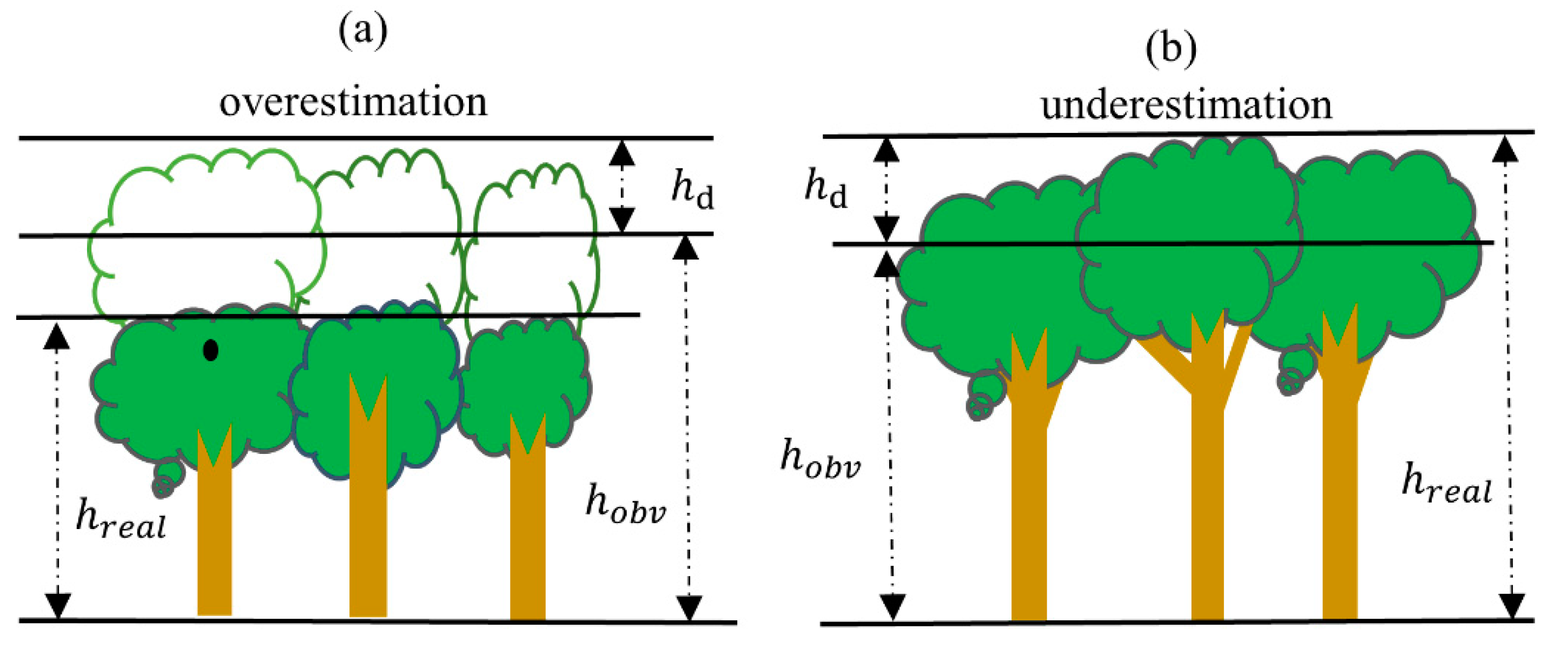
Figure 6.
Schematic illustration of underestimation and overestimation of forest canopy height.

Figure 7.
Technical workflow.

Figure 8.
Plots showing forest height validation results of RVoG model inversion in the (a) Lope and (b) Pongara test areas.
Figure 8.
Plots showing forest height validation results of RVoG model inversion in the (a) Lope and (b) Pongara test areas.

Figure 9.
Scatter plots illustrating the validation of results corrected to the reference height threshold for the (b–d) Lope test area and (f–h) Pongara test area. (a,e) are the results of the RVoG model before correction for the Lope and Pongara test areas, respectively.
Figure 9.
Scatter plots illustrating the validation of results corrected to the reference height threshold for the (b–d) Lope test area and (f–h) Pongara test area. (a,e) are the results of the RVoG model before correction for the Lope and Pongara test areas, respectively.


Figure 10.
Scatter plots of p-values vs. error and RH100 for the Lope (a,b) and Pongara (c,d) test areas.
Figure 10.
Scatter plots of p-values vs. error and RH100 for the Lope (a,b) and Pongara (c,d) test areas.

Figure 11.
Plots showing validation of the results corrected according to the P threshold in the (a–c) Lope test area and (d–f) Pongara test area.
Figure 11.
Plots showing validation of the results corrected according to the P threshold in the (a–c) Lope test area and (d–f) Pongara test area.


Figure 12.
Heat maps showing the independent variable Pearson correlation coefficient between variable pairs for the (a) Lope and (b) Pongara test areas.
Figure 12.
Heat maps showing the independent variable Pearson correlation coefficient between variable pairs for the (a) Lope and (b) Pongara test areas.

Figure 13.
Scatter plots showing the validation results of p-values as correction thresholds for the (a) Lope and (b) Pongara test areas.
Figure 13.
Scatter plots showing the validation results of p-values as correction thresholds for the (a) Lope and (b) Pongara test areas.

Figure 14.
Scatter plots showing the validation of results with PRF as a threshold correction in the Lope test area (b–d) and the Pongara test area (f–h). (a,e) are the results of the RVoG model before correction for the Lope and Pongara test areas, respectively.
Figure 14.
Scatter plots showing the validation of results with PRF as a threshold correction in the Lope test area (b–d) and the Pongara test area (f–h). (a,e) are the results of the RVoG model before correction for the Lope and Pongara test areas, respectively.

Figure 15.
Correction results based on PRF in the lope test area (a) and the Pongara test area (b).


Table 1.
Forest conditions.
| Test Area | Type of Forest | Forest Height Information (m) | ||
|---|---|---|---|---|
| Max Height | Min Height | Average Height | ||
| Lope | Inland tropical forest | 84.28 | 1.94 | 36.94 |
| Pongara | Mangrove forest | 65.11 | 1.80 | 20.71 |
Table 2.
Summary of UAVSAR data.
| Test Area | Number of Tracks | Vertical Baseline (m) | Range Resolution (m) | Azimuth Resolution (m) |
|---|---|---|---|---|
| Lope | 8 | 0, 20, 45, 105 | 3.33 | 4.8 |
| Pongara | 5 | 0, 20, 40, 60, 80, 100, 120 | 3.33 | 4.8 |
Table 3.
Iteration results based on reference height.
| Lope | Pongara | ||||||||
|---|---|---|---|---|---|---|---|---|---|
| Hi (m) | RMSE (m) | R2 | RMSE (m) | R2 | Hi (m) | RMSE (m) | R2 | RMSE (m) | R2 |
| 0.000 | 11.763 | 0.481 | 7.777 | 0.773 | 0.000 | 17.519 | −0.310 | 7.789 | 0.741 |
| 2.000 | 11.763 | 0.481 | 7.777 | 0.773 | 2.000 | 17.519 | −0.310 | 7.789 | 0.741 |
| 4.000 | 11.632 | 0.493 | 7.658 | 0.780 | 4.000 | 17.482 | −0.304 | 7.749 | 0.744 |
| 6.000 | 11.465 | 0.507 | 7.511 | 0.788 | 6.000 | 17.406 | −0.293 | 7.681 | 0.748 |
| 8.000 | 11.330 | 0.519 | 7.399 | 0.795 | 8.000 | 17.321 | −0.280 | 7.602 | 0.753 |
| 10.000 | 11.207 | 0.529 | 7.299 | 0.800 | 10.000 | 17.248 | −0.270 | 7.552 | 0.757 |
| 12.000 | 11.131 | 0.535 | 7.247 | 0.803 | 12.000 | 17.184 | −0.260 | 7.501 | 0.760 |
| 14.000 | 11.081 | 0.540 | 7.216 | 0.805 | 14.000 | 17.091 | −0.247 | 7.422 | 0.765 |
| 16.000 | 11.032 | 0.544 | 7.193 | 0.806 | 16.000 | 16.969 | −0.229 | 7.303 | 0.772 |
| 18.000 | 10.953 | 0.550 | 7.151 | 0.808 | 18.000 | 16.852 | −0.212 | 7.212 | 0.778 |
| 20.000 | 10.879 | 0.556 | 7.123 | 0.810 | 20.000 | 16.731 | −0.195 | 7.102 | 0.785 |
| 22.000 | 10.814 | 0.561 | 7.107 | 0.811 | 22.000 | 16.576 | −0.173 | 6.977 | 0.792 |
| 24.000 | 10.737 | 0.568 | 7.088 | 0.812 | 24.000 | 16.408 | −0.149 | 6.878 | 0.798 |
| 26.000 | 10.659 | 0.574 | 7.077 | 0.812 | 26.000 | 16.130 | −0.110 | 6.695 | 0.809 |
| 28.000 | 10.564 | 0.582 | 7.063 | 0.813 | 28.000 | 15.763 | −0.061 | 6.481 | 0.821 |
| 30.000 | 10.378 | 0.596 | 7.056 | 0.813 | 30.000 | 15.338 | −0.004 | 6.289 | 0.831 |
| 32.000 | 10.121 | 0.616 | 7.066 | 0.813 | 32.000 | 14.522 | 0.100 | 5.986 | 0.847 |
| 34.000 | 9.824 | 0.638 | 7.114 | 0.810 | 34.000 | 13.709 | 0.198 | 5.839 | 0.854 |
| 36.000 | 9.427 | 0.667 | 7.239 | 0.804 | 36.000 | 12.866 | 0.293 | 5.909 | 0.851 |
| 38.000 | 8.957 | 0.699 | 7.590 | 0.784 | 38.000 | 11.912 | 0.394 | 6.061 | 0.843 |
| 40.000 | 8.380 | 0.737 | 8.255 | 0.744 | 40.000 | 10.841 | 0.498 | 6.386 | 0.826 |
| 42.000 | 7.691 | 0.778 | 9.332 | 0.673 | 42.000 | 9.991 | 0.574 | 6.746 | 0.806 |
| 44.000 | 7.121 | 0.810 | 10.669 | 0.573 | 44.000 | 9.181 | 0.640 | 7.203 | 0.779 |
| 46.000 | 6.995 | 0.817 | 11.873 | 0.471 | 46.000 | 8.613 | 0.683 | 7.613 | 0.753 |
| 48.000 | 7.225 | 0.804 | 13.009 | 0.365 | 48.000 | 8.236 | 0.710 | 8.049 | 0.723 |
| 50.000 | 7.420 | 0.794 | 13.625 | 0.304 | 50.000 | 7.843 | 0.737 | 8.495 | 0.692 |
| 52.000 | 7.562 | 0.786 | 13.954 | 0.270 | 52.000 | 7.760 | 0.743 | 8.910 | 0.661 |
| 54.000 | 7.667 | 0.780 | 14.118 | 0.253 | 54.000 | 7.743 | 0.744 | 9.102 | 0.646 |
| 56.000 | 7.729 | 0.776 | 14.196 | 0.244 | 56.000 | 7.748 | 0.744 | 9.265 | 0.634 |
| 58.000 | 7.763 | 0.774 | 14.233 | 0.240 | 58.000 | 7.773 | 0.742 | 9.339 | 0.628 |
| 60.000 | 7.777 | 0.773 | 14.252 | 0.238 | 60.000 | 7.789 | 0.741 | 9.385 | 0.624 |
| 62.000 | 7.777 | 0.773 | 14.252 | 0.238 | 62.000 | 7.789 | 0.741 | 9.385 | 0.624 |
| 64.000 | 7.777 | 0.773 | 14.252 | 0.238 | 64.000 | 7.789 | 0.741 | 9.385 | 0.624 |
| 66.000 | 7.777 | 0.773 | 14.252 | 0.238 | 66.000 | 7.789 | 0.741 | 9.385 | 0.624 |
Table 4.
Iteration results based on p-values.
| Lope | Pongara | ||||||||
|---|---|---|---|---|---|---|---|---|---|
| Pi | RMSE (m) | R2 | RMSE (m) | R2 | P | RMSE (m) | R2 | RMSE (m) | R2 |
| 0.000 | 11.763 | 0.481 | 7.777 | 0.773 | 0.000 | 17.519 | −0.310 | 7.789 | 0.741 |
| 0.200 | 11.763 | 0.481 | 7.777 | 0.773 | 0.200 | 17.519 | −0.310 | 7.789 | 0.741 |
| 0.400 | 11.763 | 0.481 | 7.777 | 0.773 | 0.400 | 17.519 | −0.310 | 7.789 | 0.741 |
| 0.600 | 11.726 | 0.484 | 7.741 | 0.775 | 0.600 | 17.516 | −0.309 | 7.785 | 0.741 |
| 0.800 | 11.670 | 0.489 | 7.683 | 0.779 | 0.800 | 17.477 | −0.304 | 7.733 | 0.745 |
| 1.000 | 11.584 | 0.497 | 7.600 | 0.783 | 1.000 | 17.440 | −0.298 | 7.684 | 0.748 |
| 1.200 | 11.465 | 0.507 | 7.491 | 0.790 | 1.200 | 17.313 | −0.279 | 7.541 | 0.757 |
| 1.400 | 11.320 | 0.520 | 7.365 | 0.797 | 1.400 | 17.091 | −0.247 | 7.305 | 0.772 |
| 1.600 | 11.191 | 0.530 | 7.260 | 0.802 | 1.600 | 16.767 | −0.200 | 6.991 | 0.791 |
| 1.800 | 11.097 | 0.538 | 7.191 | 0.806 | 1.800 | 16.258 | −0.128 | 6.627 | 0.813 |
| 2.000 | 10.979 | 0.548 | 7.123 | 0.810 | 2.000 | 15.463 | −0.020 | 6.134 | 0.839 |
| 2.200 | 10.736 | 0.568 | 7.010 | 0.816 | 2.200 | 14.381 | 0.117 | 5.631 | 0.865 |
| 2.400 | 10.442 | 0.591 | 6.914 | 0.821 | 2.400 | 13.024 | 0.276 | 5.308 | 0.880 |
| 2.600 | 9.955 | 0.628 | 6.877 | 0.823 | 2.600 | 11.718 | 0.414 | 5.339 | 0.878 |
| 2.800 | 9.305 | 0.675 | 7.040 | 0.814 | 2.800 | 10.042 | 0.570 | 5.750 | 0.859 |
| 3.000 | 8.423 | 0.734 | 7.438 | 0.793 | 3.000 | 8.852 | 0.666 | 6.504 | 0.819 |
| 3.200 | 7.481 | 0.790 | 8.116 | 0.753 | 3.200 | 8.048 | 0.724 | 7.306 | 0.772 |
| 3.400 | 6.623 | 0.836 | 9.152 | 0.686 | 3.400 | 7.693 | 0.747 | 7.838 | 0.738 |
| 3.600 | 6.126 | 0.859 | 10.268 | 0.605 | 3.600 | 7.562 | 0.756 | 8.302 | 0.706 |
| 3.800 | 5.996 | 0.865 | 11.257 | 0.525 | 3.800 | 7.531 | 0.758 | 8.598 | 0.684 |
| 4.000 | 6.128 | 0.859 | 12.031 | 0.457 | 4.000 | 7.539 | 0.757 | 8.842 | 0.666 |
| 4.200 | 6.378 | 0.847 | 12.603 | 0.404 | 4.200 | 7.572 | 0.755 | 8.983 | 0.656 |
| 4.400 | 6.625 | 0.835 | 13.011 | 0.365 | 4.400 | 7.598 | 0.754 | 9.064 | 0.649 |
| 4.600 | 6.837 | 0.825 | 13.306 | 0.336 | 4.600 | 7.638 | 0.751 | 9.156 | 0.642 |
| 4.800 | 7.055 | 0.813 | 13.572 | 0.309 | 4.800 | 7.653 | 0.750 | 9.185 | 0.640 |
| 5.000 | 7.188 | 0.806 | 13.730 | 0.293 | 5.000 | 7.675 | 0.749 | 9.225 | 0.637 |
| 5.200 | 7.304 | 0.800 | 13.854 | 0.280 | 5.200 | 7.695 | 0.747 | 9.257 | 0.634 |
| 5.400 | 7.403 | 0.794 | 13.947 | 0.271 | 5.400 | 7.724 | 0.745 | 9.298 | 0.631 |
| 5.600 | 7.489 | 0.790 | 14.023 | 0.263 | 5.600 | 7.743 | 0.744 | 9.326 | 0.629 |
| 5.800 | 7.541 | 0.787 | 14.069 | 0.258 | 5.800 | 7.757 | 0.743 | 9.346 | 0.627 |
| 6.000 | 7.575 | 0.785 | 14.099 | 0.255 | 6.000 | 7.763 | 0.743 | 9.353 | 0.627 |
| 6.200 | 7.602 | 0.783 | 14.121 | 0.252 | 6.200 | 7.776 | 0.742 | 9.369 | 0.625 |
| 6.400 | 7.633 | 0.782 | 14.145 | 0.250 | 6.400 | 7.783 | 0.741 | 9.377 | 0.625 |
| 6.600 | 7.658 | 0.780 | 14.164 | 0.248 | 6.600 | 7.783 | 0.741 | 9.377 | 0.625 |
| 6.800 | 7.685 | 0.779 | 14.185 | 0.246 | 6.800 | 7.789 | 0.741 | 9.385 | 0.624 |
| 7.000 | 7.718 | 0.777 | 14.210 | 0.243 | 7.000 | 7.789 | 0.741 | 9.385 | 0.624 |
| 7.200 | 7.727 | 0.776 | 14.217 | 0.242 | 7.200 | 7.789 | 0.741 | 9.385 | 0.624 |
| 7.400 | 7.727 | 0.776 | 14.217 | 0.242 | 7.400 | 7.789 | 0.741 | 9.385 | 0.624 |
| 7.600 | 7.735 | 0.776 | 14.223 | 0.242 | 7.600 | 7.789 | 0.741 | 9.385 | 0.624 |
| 7.800 | 7.754 | 0.775 | 14.236 | 0.240 | 7.800 | 7.789 | 0.741 | 9.385 | 0.624 |
| 8.000 | 7.765 | 0.774 | 14.243 | 0.239 | 8.000 | 7.789 | 0.741 | 9.385 | 0.624 |
| 8.200 | 7.773 | 0.773 | 14.249 | 0.239 | |||||
| 8.400 | 7.777 | 0.773 | 14.252 | 0.238 | |||||
| 8.600 | 7.777 | 0.773 | 14.252 | 0.238 | |||||
| 8.800 | 7.777 | 0.773 | 14.252 | 0.238 | |||||
| 9.000 | 7.777 | 0.773 | 14.252 | 0.238 | |||||
Table 5.
List of independent variables used in machine learning methods.
| Variable Type | Name | Description | Expressions |
|---|---|---|---|
| Geometric parameters | Cos θ | Incident angle cosine | None |
| Sin θ | Incident angle sine | None | |
| Inc | Incident angle | None | |
| Kz | Vertical wave number | / | |
| HoA | Height of ambiguity | ||
| Penetration depth | Hd | Penetration depth | / |
| Coherence phase center height and coherence separation | PDHsep | High-coherence separation | |
| PDLsep | Low-coherence separation | ||
| PDHmab | High-coherence magnitude | ||
| PDLmab | Low-coherence amplitude | ||
| PDHarg | High-coherence phases | ||
| PDLarg | Low-coherence phases | ||
| Phi | Ground phase | / | |
| Phimab | Surface coherence amplitude | ||
| HeightPDH | High-coherence phase center height | ||
| HeightPDL | Low-coherence phase center height | ||
| Baseline selection parameters | Sep | Coherence separation | |
| Mab | Coherence amplitude | ||
| Cit | Product of coherence separation and coherence amplitude |
Table 6.
Comparison of the results of different correction schemes.
| Correction Scheme | Test Area | R2 | RMSE (m) | BIAS (m) |
|---|---|---|---|---|
| Uncorrected | Lope | 0.775 | 7.748 | 1.120 |
| Pongara | 0.752 | 7.628 | −4.188 | |
| Correction based on RH100 | Lope | 0.856 | 6.204 | 0.536 |
| Pongara | 0.854 | 5.856 | −0.024 | |
| Correction based on P | Lope | 0.914 | 4.796 | 0.011 |
| Pongara | 0.896 | 4.939 | −0.834 | |
| Correction based on PRF | Lope | 0.845 | 6.422 | 0.209 |
| Pongara | 0.780 | 7.184 | −2.035 |
Publisher’s Note: MDPI stays neutral with regard to jurisdictional claims in published maps and institutional affiliations. |
© 2022 by the authors. Licensee MDPI, Basel, Switzerland. This article is an open access article distributed under the terms and conditions of the Creative Commons Attribution (CC BY) license (https://creativecommons.org/licenses/by/4.0/).
Share and Cite
MDPI and ACS Style
Luo, H.; Yue, C.; Wang, N.; Luo, G.; Chen, S. Correcting Underestimation and Overestimation in PolInSAR Forest Canopy Height Estimation Using Microwave Penetration Depth. Remote Sens. 2022, 14, 6145. https://doi.org/10.3390/rs14236145
AMA Style
Luo H, Yue C, Wang N, Luo G, Chen S. Correcting Underestimation and Overestimation in PolInSAR Forest Canopy Height Estimation Using Microwave Penetration Depth. Remote Sensing. 2022; 14(23):6145. https://doi.org/10.3390/rs14236145
Chicago/Turabian StyleLuo, Hongbin, Cairong Yue, Ning Wang, Guangfei Luo, and Si Chen. 2022. "Correcting Underestimation and Overestimation in PolInSAR Forest Canopy Height Estimation Using Microwave Penetration Depth" Remote Sensing 14, no. 23: 6145. https://doi.org/10.3390/rs14236145
Note that from the first issue of 2016, this journal uses article numbers instead of page numbers. See further details here.