
Increased Ice Thinning over Svalbard Measured by ICESat/ICESat-2 Laser Altimetry


Institute of Geography, Friedrich-Alexander-Universität Erlangen-Nürnberg, 91052 Erlangen, Germany
*
Author to whom correspondence should be addressed.
Remote Sens. 2021, 13(11), 2089; https://doi.org/10.3390/rs13112089
Submission received: 13 April 2021
/
Revised: 19 May 2021
/
Accepted: 20 May 2021
/
Published: 26 May 2021
(This article belongs to the Special Issue Satellite Altimetry: Technology and Application in Geodesy)
Abstract
:A decade-long pronounced increase in temperatures in the Arctic, especially in the Barents Sea region, resulted in a global warming hotspot over Svalbard. Associated changes in the cryosphere are the consequence and lead to a demand for monitoring of the glacier changes. This study uses spaceborne laser altimetry data from the ICESat and ICESat-2 missions to obtain ice elevation and mass change rates between 2003–2008 and 2019. Elevation changes are derived at orbit crossover locations throughout the study area, and regional volume and mass changes are estimated using a hypsometric approach. A Svalbard-wide annual elevation change rate of −0.30 ± 0.15 m yr−1 was found, which corresponds to a mass loss rate of −12.40 ± 4.28 Gt yr−1. Compared to the ICESat period (2003–2009), thinning has increased over most regions, including the highest negative rates along the west coast and areas bordering the Barents Sea. The overall negative regime is expected to be linked to Arctic warming in the last decades and associated changes in glacier climatic mass balance. Further, observed increased thinning rates and pronounced changes at the eastern side of Svalbard since the ICESat period are found to correlate with atmospheric and oceanic warming in the respective regions.
Keywords:
ICESat; ICESat-2; laser; altimetry; svalbard; barents sea; geodesy; glacier; ice cap; elevation change; mass change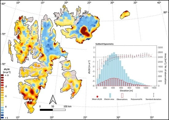
1. Introduction
Observing variances in global cryosphere characteristics remains an important factor in a warming climate. Consequently, several satellite-mounted laser and radar sensors have been used to continuously measure surface elevation change of glacier and ice caps in the last decades (e.g., [1,2,3,4,5]). While radar systems typically exhibit a large footprint of several meters to kilometers and can penetrate into ice, snow, and firn (e.g., [6]), the advantages of laser altimetry lie in a small footprint of cm to meters and in the measurement of precise surface heights with little subsurface penetration. Glacier topography investigations with laser altimeters were initially mainly conducted through aircraft campaigns (e.g., [7,8]) until NASA launched its first spaceborne satellite laser altimetry mission ICESat (Ice, Cloud, and Land Elevation Satellite), which operated between 2003–2009. The mission data has been successfully used for glacier mass change estimates in non-polar (e.g., [9]) and polar (e.g., [10]) regions. In 2018, its successor, ICESat-2, was launched equipped with an improved laser altimetry system, which is expected to produce height measurements with enhanced accuracy and coverage (e.g., [11]). The first data analyses have shown its potential for cryosphere applications, such as mapping of grounding lines in Antarctica [12] or elevation and mass change assessments for the Greenland and Antarctic ice sheets [11]. However, for smaller glaciated regions like Svalbard, an evaluation of the potential of combining data from both missions through a crossover approach has not been published yet.
In terms of Arctic amplification, the Barents Sea area represents an inter-Arctic warming hotspot [13,14]. Because it is located at the western border of this fast-warming region and at an area of retreating Arctic sea ice, the ice caps and glaciers of Svalbard are exposed to the fastest warming on Earth [15]. An accompanied significant reduction in glacier area and mass balance through the 21st century is expected [16], which makes an investigation of recent elevation and mass change patterns indispensable. Simulations have already shown negative surface mass balance and mass loss since the 1980s at variable rates [15,17,18], which is supported by several remote-sensing based negative elevation and mass change estimates over the last decades [19,20,21]. Therefore, the aim of this study is to evaluate the potential of ICESat and ICESat-2 data in Svalbard to determine elevation and mass change trends in the period of 2003–2008 to 2019. The derived ICESat/ICESat-2 change trends are compared to recent CryoSat-2 results between 2011–2017 [19], and observed alterations relative to 2003–2008 intra-ICESat acquisitions [20] are discussed. The assessment of the used technique to derive ICESat/ICESat-2 results is provided through an in-depth analysis of the performance over Svalbard. In support of recent radar altimetry measurements [19], this use of precise laser acquisitions by ICESat/ICESat-2, with its unique properties, is expected to deliver detailed insights of elevation and mass change patterns in one of the most critical environments regarding climate change.
2. Study Area
Svalbard is an Arctic archipelago located north of Norway between 75–82 °N (Figure 1). It is surrounded by the northern Atlantic Ocean to the south and the Arctic Ocean to the north. The western parts of the six major islands are mostly influenced by the warm West Spitsbergen Current, whereas the eastern part is impacted by clearly cooler waters from the Arctic Ocean [22]. Due to the location at the junction of northern cold and dry polar air masses and southwestern warm and humid air masses from the Atlantic currents, meteorological conditions are spatially and temporally versatile [20]. Overall, the archipelago is characterized by strong climate gradients, including milder and more humid conditions in the south and west, and colder and drier conditions in the northeast [23].
The ice masses in Svalbard consist mainly of ice caps, which cover most of the land mass of Nordaustlandet and Kvitøya, and extensive ice fields on the interiors of Spitsbergen and Barentsøya/Edgeøya. Svalbard covers a total area of ~60,000 km2 [23], from which 57% or ~34,000 km2 are covered with glaciers [24]. This corresponds to ~10% of the glaciers in the Arctic outside the Greenland ice sheet [23] and represents 6% of the worldwide Glacier coverage outside Antarctica and Greenland [20]. Recent estimates about total ice volume agree on ~6200 km3 or a sea-level equivalent of 1.5 cm [25,26]. Of all glaciers, 15% by number [23] and up to 60% by area [27] are tidewater glaciers terminating into fjord or ocean water [23]. Overall, glaciers are mainly polythermal, thus consisting of cold and temperate ice [23]. They have typically shown slow velocities of 2–10 m yr−1 [28] and a negative surface-mass balance and mass loss at variable rates since the 1980s [15,17,18], supported by several remote-sensing based negative elevation and mass change estimates over the last decades [19,20,21]. Contrasting other Arctic glaciers, Svalbard’s ice masses exhibit a low maximum of area-elevation distribution at ~450 m a.s.l., compared to ice caps of, for example, Greenland, Arctic Canada, and Iceland, which have corresponding altitudes between ~800–1400 m a.s.l. [15]. With a proportion of 60%, most of the ice is located under this rather low hypsometric peak. Additionally, they are very vulnerable to changes in atmospheric temperatures because the equilibrium-line-altitude fluctuates around that peak [15].
Surging behavior is common over the archipelago. Most reported surging glaciers are located in southern Spitsbergen (~45%), while the rest is equally distributed over the other regions [29]. The overall proportion of surging glaciers is uncertain and estimates to range from 13% to 90% of all glaciers [29,30]. Overall, 345 surge-type glaciers have been identified until 2013 [31]. The quiescence phase in Svalbard typically lasts between 30–500 [32] years and is followed by an active (surging) phase ranging between 3–10 years [30,32]. This is much longer than for surge-type glaciers in for example, North America, Iceland, and the Pamirs, where active phases only last 1 to 2 years [30].
3. ICESat and ICESat-2
ICESat was launched on 12 January 2003 and ended its operation after seven years [33]. The payload included the ‘Geoscience Laser Altimeter System’ (GLAS), which contained three 1064 nm laser altimeters with a laser pointing angle determination system and a 1064/532 nm cloud and aerosol LIDAR (light detection and ranging) [34]. While operating, each laser pulsed at 40 Hz and illuminated a spot of about 65 m in diameter on the earth’s surface, whereas individual spots are separated by 172 m in along-track direction [3]. GLAS measurements were found to have a <3 cm shot-to-shot precision over ice sheets, which significantly improved the accuracy of elevation measurements over such surfaces [34]. On 29 March 2003 Laser 1 failed and caused an adaption to several month-long measurement campaigns [3,34]. This reduced the GLAS operation time by 73% [34]. Hence, during the whole mission, the adopted 33 to 56-day campaign plan was used to extend the ICESat mission lifetime [35].
Its successor, ICESat-2, was successfully launched on 15th September 2018 [36] and carries the Advanced Topographic Laser Altimetry System (ATLAS) instrument. ATLAS uses a photon-counting LIDAR instrument to measure the time a photon needs from ATLAS to the earth and back, the pointing vector at the time a photon is transmitted, and the position of ICESat-2 in space at the time a photon is recorded [37]. ATLAS transmits green (532 nm) laser pulses at 10 kHz and splits each laser pulse by a diffractive optical element to generate six individual beams in three pairs. The beams in a pair have different transmit energies (energy ration of ~1:4) and are separated by 90 m in the across-track direction. Individual pairs are separated by ~3.3 km in the across-track direction, and strong and weak beams are separated by ~2.5 km in the along-track direction [37]. Through firing at 10 kHz from a nominal ~500 km orbit height, a laser pulse is transmitted every ~0.7 m in along-track direction for each beam [37]. This ensures minimal measurement gaps and provides a higher fidelity of topography, even over rough and heterogeneous glacier and sea surfaces [38]. With this high sampling rate, a narrow footprint of ~14.5 m, and a near global coverage (+/−88° latitude), the mission is designed to repeatedly measure the ice sheets by revisiting 1387 reference ground tracks with a 10 m horizontal accuracy and 0.03 m vertical precision every 91 days [11].
4. Materials and Methods
The extraction of change signals from ICESat laser altimetry is typically performed by many different techniques (e.g., [20,39,40,41,42]). In this study, orbit crossover locations of the ICESat and ICESat-2 missions were used to compare height values measured by both systems at those positions. Some processing steps were thereby performed using NASA’s cryosphere altimetry processing toolkit ‘captoolkit’ by F. Paolo, J. Nilsson, A. Gardner, and T. Sutterly (https://github.com/fspaolo/captoolkit (access on 1 April 2020)). This tool provides a collection of editable Python scripts for many purposes regarding laser and radar altimetry. The crossover method is additionally tested in comparison to common intra-ICESat repeat-track analysis over a test ground track in Vestfonna, which is provided in the Supplementary Materials.
4.1. Data Preparation
For ICESat, the GLAS/ICESat L1B Global Elevation Data GLAH06 Release 634 of the National Snow & Ice Data Center (NSIDC) was used between 2003 and 2008. Some corrections were applied to the GLAH06 data, including a detector saturation correction [43] and an inter-laser bias correction for ICESat’s laser 2 and 3 [44]. Together with those major corrections, data culling, and general corrections for ICESat data were carried out as follows:
- Sorted out data not meeting the on-product variable criteria: ‘elev_use_flg == 0’, ‘sat_corr_flg < = 2’, ‘sigma_att_flag == 0’, and ‘i_numPk == 1’;
- Applied the saturation correction;
- Converted from the Topex/Poseidon ellipsoidal height to WGS84 ellipsoidal height;
- Applied the inter-laser correction: subtracting 1.7 cm from Laser 2 and adding 1.1 cm to Laser 3 according to [11] due to the same methodological approach.
Data preparation was achieved for all ICESat high energy spring campaigns (L1A, L2B, L3B, L3E, L3H, L3J), which makes a total of six campaigns from 2003 to 2008. Only spring campaigns were chosen to minimize seasonal effects.
ICESat-2 data came from the ATLAS/ICESat-2 L3A Land Ice Height ATL06 Version 3 dataset by NSIDC. ATL06 data were produced with a special segmentation technique: along-track geolocated ATL03 photon data from each beam were divided into 40 m long overlapping (20 m) segments, followed by fitting photon heights with a linear model as a function of along-track distance [11]. Data were finally corrected for instrument specific deviations, such as first-photon bias and transmit-pulse shape, which produced the final ATL06 product. This includes latitude, longitude, and height, with respect to the WGS84 ellipsoid for each segment [11]. ATL06 data from 14th January 2019 to 14th April 2019 were used to ensure coverage of the complete ICESat spring campaign months while using all measurements of a full 91-day repeat cycle. Data were filtered similar to [11], as follows:
- Removed data flagged by the on-product ATL06 quality summary value;
- Removed data where adjacent segment height differences were >2 m and therefore exhibited high along-track height variability;
- Removed data where surface height was >10,000 m due to atmospheric scattering.
4.2. ICESat-1/2 Crossover Analysis
Crossover locations were determined between all six ICESat spring campaigns and the 2019 ICESat-2 spring dataset. Due to the 6-beam architecture of ATLAS, crossing of one ground track from ICESat with the tracks of ICESat-2 produced up to six crossovers. To calculate orbit intersections, latitude and longitude values projected in UTM Zone 35N for all footprints of always one ICESat-2 track were inserted into geometric functions with all measurements from always one track of ICESat (Figure 2). This was repeated until each ICESat-2 track was compared with every ICESat track. The algorithm was implemented by the authors of the ‘captoolkit’ and produced the exact location of intersections between all used ICESat/ICESat-2 tracks. After a crossover location was determined, it was checked if one of the four nearest footprints exceeded the threshold of 350 m distance to the crossing position. If so, the crossover value was not used in the analysis. Because of the larger distance between individual ICESat footprints, this allowed for one ICESat measurement to be missing, even if the neighboring footprint was close to the orbit intersection. Next, the height data of the four measurements were linearly interpolated to the crossing position and both interpolated elevation values were subtracted from each other. dh/dt values were finally calculated by dividing the absolute elevation change values through the timespan between the two acquisitions (between ~11 to ~16 years). The calculation of such annual elevation change time series (dh/dt) allows for the comparison of elevation change values between the six ICESat campaigns and the ICESat-2 acquisitions. In total, 8822 crossovers were found between all datasets.
4.3. Hypsometric Extrapolation
Despite achieving up to six elevation change measurements between one orbit crossing, the spatial extent of the crossovers is still mostly limited to the ICESat reference tracks. Since data coverage is therefore too sparse to determine total change rates through local spatial interpolation, especially in mountainous terrain in NW and NE [20], a hypsometric approach similar to [20,21], was used to estimate ice volume and mass changes. At first, the data were separated into the different regions presented in Figure 1. Next, dh/dt values were split by the surface heights at the crossover locations into 50 m elevation bins for every region. All dh/dt values for each bin were then filtered by excluding all values which exceed the threshold of three times the mean absolute deviation from the median of all values. After filtering, 8021 valid crossover points were left, excluding general outliers and some extreme values through surging events. To derive annual volume changes, 50 m glacier hypsometries were determined by the 20 m resolution ‘S0_DTM20_NP-ArcticDEM-Mosaic’ Svalbard digital elevation model from the Norwegian Polar Institute (NPI) [45]. The DEM is an updated version of the ‘S0_Terrengmodell’ from 2014 and includes more recent data [46]. The original DEM was mostly processed using stereo models from aerial photos and from elevation contours, lakes, and coastlines [47]. Data from the ‘Randolph Glacier Inventory 6.0’ (RGI) [48] served as a mask to clip the DEM to only glaciated regions. Glacier areas were calculated for each region by counting the cells in the model per 50 m bin (e.g., in 100–150 m altitude) and multiplying the number of cells by their median size. A third order polynomial curve was fit to the mean of all dh/dt values for every elevation bin per region (Figure 3). This is required to fill bins which are lacking dh/dt measurements but have glacier area values.
Extrapolation of measurements to unsurveyed areas with polynomial fits are a common practice in laser (e.g., [20,21]) and radar (e.g., [19]) investigations. In this context, the usage of third order polynomial fits in this study allows for a direct comparison with the hypsometries derived from ICESat by Moholdt et al. [20] and CryoSat-2 by Morris et al. [19]. The third order polynomial fit can produce runaway tails at the data edge, however, as bins which are filled with the polynomial value typically correspond to just one bin with an area proportion ranging between 0.11–0.99% of the total regional area value, their contribution to volume change calculations is neglectable. Storisstraumen is an exception with 8.77% of total area filled with polynomial fits, which is still expected to have just a minor impact on calculations. Using the mean dh/dt value with fits per bin or just polynomial values resulted in no significant difference in final results. For example, the total Svalbard mass loss rate (dM/dt2) calculated with mean dh/dt and fit values was −12.21 ± 4.28 Gt yr−1, compared to −12.19 ± 4.28 Gt yr−1, by using just polynomial fit values.
Annual volume change (dV/dt in m3) for each region was finally calculated using the following equation:
where n is the number of 50 m bins per region, h is the mean of all dh/dt measurements in m yr−1, or (if missing) the polynomial fit, and A is the glacier area in m2 per bin i. Averaged elevation change rates dh/dt were then calculated by dividing the dV/dt value of each region by the corresponding total Glacier area A. Further, mass loss rates were determined by multiplying dV/dt with the density of ice (0.917 g/cm3, dM/dt1) and additionally with a density of 0.850 g/cm3 (dM/dt2) to partly include changes in the firn pack. The conversion factor for dM/dt2 was chosen based on the suggestions of Huss et al. [49] for periods > 5 years by assuming stable mass balance gradients, the presence of a firn area, and volume changes significantly other than zero. Due to the large spatial extent and extreme dh/dt values through a surging event [50], acquisitions over the Storisstraumen Glacier in Austfonna were treated separately. Values for Austfonna were subsequently estimated without the contribution from the glacier basin, whereas mass loss contribution from the surge is discussed in Section 6.2. The final Svalbard-wide mass change value is the sum of all regional dM/dt2 estimates and the dM/dt1 value for Storisstraumen, assuming that the mass loss from this basin was mainly caused by surging ice. The total thinning rate was determined by using all regional filtered crossover values excluding Storisstraumen and corresponding total bin area values. Further, despite the spatial relative limited data, ordinary kriging interpolation was performed with all crossover measurements (including Storisstraumen) to produce an approximate spatial overview of elevation change trends over Svalbard (Figure 4). For this purpose, a grid with a 1 km2 resolution was roughly cropped to the outline of the RGI, and an experimental variogram based on all crossover values was computed. Next, a spherical model with a range of ~30, sill of ~1.1, and nugget of ~0.05 as parameter settings was fitted to the variogram, and all dh/dt values were finally interpolated over the grid, based on this model.
4.4. Error Assessment
Over non-glaciated areas, such as rocky, solid terrain, the surface elevation was not expected to change over time. Hence, dh/dt values at ICESat/ICESat-2 orbit intersections over stable ground were expected to be zero. With this assumption, the crossover-error was estimated by crossing all ICESat campaigns with the ICESat-2 data over ice-free ground. This error assessment approach over non-glaciated terrain is common in geodetic glacier mass balance approaches and was used by [21] over Svalbard with ICESat data. For every region, is determined by calculating the root mean square error (RMSE) of all calculated values (dh/dt at crossover locations over ice-free ground) relative to the assumed elevation change of 0 m yr−1 through the following equation:
where n and N are the number of crossovers over ice-free ground for every region, and is the dh/dt value in m yr−1 at a crossover location i. After filtering all region-wide values with the threshold defined in Section 4.3, 3870 crossovers over stable ground produced error estimates ranging from 0.09 m yr−1 in Austfonna to 0.21 m yr−1 in northwest Spitsbergen. The Svalbard-wide error is 0.15 m yr−1 by calculating the area weighted mean value of all regional error estimates. Due to the very sparse non-glaciated area in Kvitøya, no crossovers on stable ground exist, and the error for Austfonna is applied in further processing steps. For Storisstraumen, the error of Austfonna was likewise applied. A previous Svalbard-wide mean crossover error of 0.20 m yr−1 was calculated within individual ICESat campaigns over ice where again only small elevation changes were expected [20]. The ICESat/ICESat-2 crossover error was consequently smaller in all regions except northwest Spitsbergen and reduced for the whole of Svalbard compared to this intra-ICESat crossover error. Regional and Svalbard-wide volume error estimates were determined by multiplying the respective values with the corresponding glaciated area values, and mass change errors were further calculated by applying the conversion factors for dM/dt1 and dM/dt2.
5. Results
Figure 4 shows 2003–2008 to 2019 spatial annual elevation change rates (dh/dt) over all of Svalbard. In Table 1, regional and Svalbard-wide elevation, volume, and mass change values are presented. The estimated Svalbard-wide dh/dt value is −0.30 ± 0.15 m yr−1, including highest rates at South Spitsbergen with −0.80 ± 0.18 m yr−1 and lowest elevation change at Austfonna and northeast Spitsbergen with −0.07 ± 0.09 m yr−1 and −0.07 ± 0.16 m yr−1, respectively (Table 1). At low altitudes (<300 m), frontal thinning is observable over all regions in the magnitude of ~0.5–5 m yr−1. Vestfonna on the other hand, experienced only slight low elevation thinning. At higher altitudes, dh/dt values tend to get more positive, but with variations, from diminished thinning at, for example, South Spitsbergen, to thickening in northeast Spitsbergen and Austfonna up to ~0.5 m yr−1. Despite the elevation decrease at the margins, this thickening trend is clearly evident in the interior Glacier and ice cap areas of Austfonna and northeast Spitsbergen. By excluding Kvitøya, a Southwest-northeast gradient is visible, specified by pronounced thinning in northwest Spitsbergen, South Spitsbergen, Barentsøya/Edgeøya, and less elevation decrease in northeast Spitsbergen, Austfonna, and Vestfonna. Overall, all regions show negative total dh/dt values, although error consideration could lead to estimates of balance for Austfonna, Vestfonna, and northeast Spitsbergen. Extreme thinning rates are especially notable (up to 10 m yr−1) over Storisstraumen in Austfonna, and are related to a surging event during the observation period [50].
5.1. Regional Elevation Change
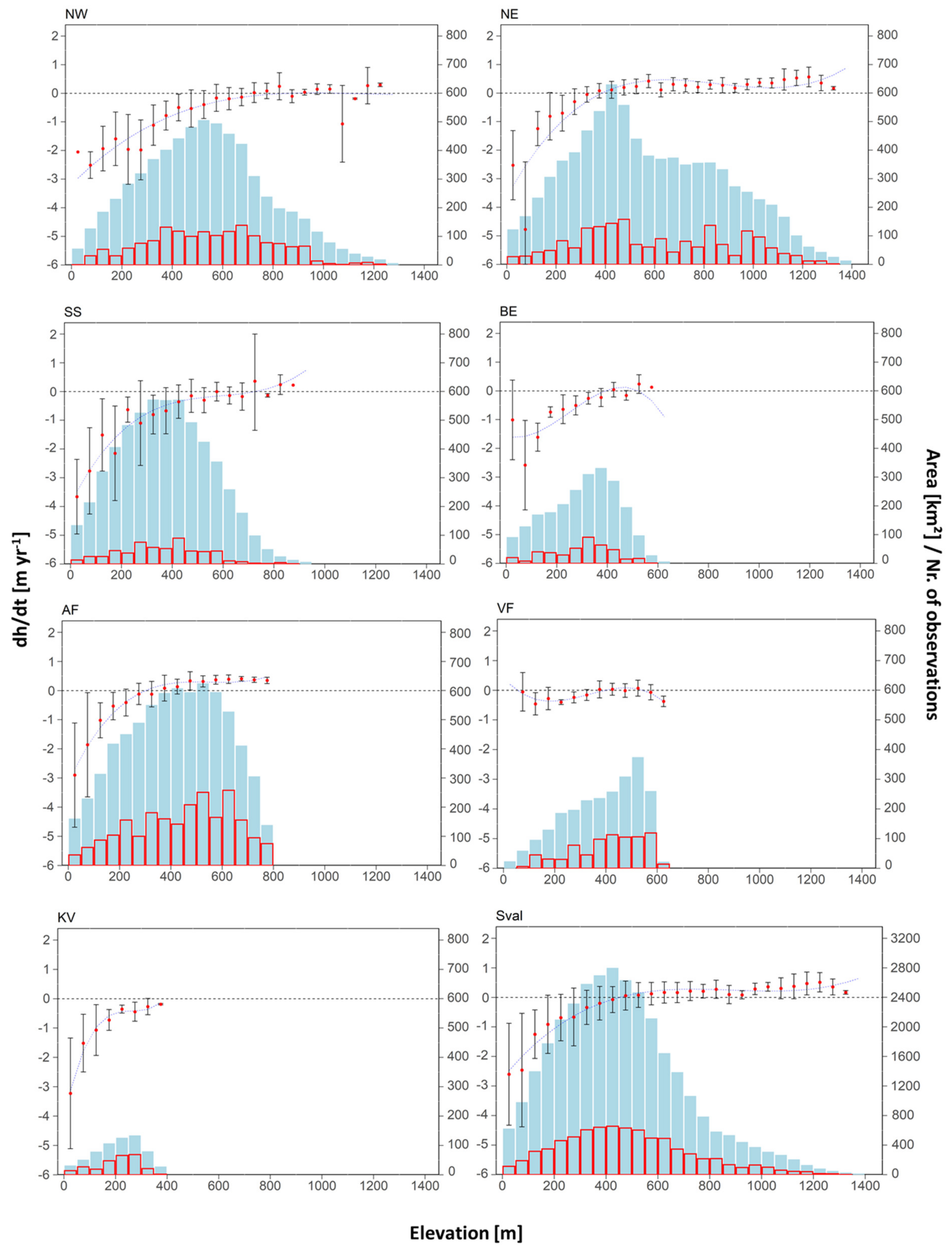
Northwest Spitsbergen has an overall high annual thinning rate of 0.63 ± 0.21 m yr−1, in addition to the significant thinning rate of ~2 m yr−1 in low altitudes (Figure 3). Only slight thickening <0.5 m yr−1 is measured at higher altitudes >700 m in the interior, where Glacier area is small. The highest negative dh/dt values can be found at the calving fronts of marine terminating glaciers, such as in the Trollheimen region in the south or Albert-I-Land in the north (Figure 4).
Northeast Spitsbergen exhibits much less elevation decrease and additional thickening at elevations >350 m up to ~0.5 m yr−1. The overall negative dh/dt estimate of −0.07 ± 0.16 m yr−1 for the whole region results from thinning rates as high as ~5 m yr−1 in combination with relatively large glacier area distribution at low altitudes. In contrast, thickening in higher altitudes is taking place at a much smaller magnitude. Negative values are spatially mostly present at the margins, and highest decrease rates can be found e.g., around the marine-terminating Oslobreen and Kongsfonna/Hachstetterbreen Glacier in the east.
With 0.80 ± 0.18 m yr−1, South Spitsbergen experienced the highest thinning rates of the whole archipelago, including an elevation decrease of up to ~−4 m yr−1 at low altitudes and overall thinning at almost all elevations. Exceptions of minor thickening are only measured at some elevations >700 m. Hotspots of decrease are found in the Wedel Jarlsberg Land region in the south, especially for example, at the Nathorstbreen Glacier system and around the Strongbreen in the east.
At the Barentsøya/Edgeøya islands, measured thinning of up to ~3 m yr−1 is found at elevations high as 400 m. Glacier area is mostly distributed up to this threshold, which results in a high regional overall decrease value of −0.54 ± 0.13 m yr−1. Slight thickening in higher altitudes is mainly found in the interior of both islands.
Next to northeast Spitsbergen, Austfonna experiences the smallest overall thinning rate of −0.07 ± 0.09 m yr−1, but with thinning up to almost 3 m yr−1 at elevations under 350 m and thickening of up to ~0.5 m yr−1 above. Positive dh/dt values can be found in the interior of the ice cap, while thinning is limited to the margins, especially in the east and south. As stated before, extreme dh/dt values of up to −10 m yr−1 are measured over Storisstraumen, thus distorting the overall pattern of thickening in the interior and thinning at the edges.
Vestfonna also shows a small elevation decrease rate of −0.09 ± 0.12 m yr−1, including the least losses or minor thickening at elevations with the largest glacier area. In the north, thickening takes places in contrast to slight thinning up to ~0.5 m yr−1 in the south.
The island Kvitøya in the northeast exhibits thinning over the complete ice cap, pronounced at the margins, which is specified by elevation decrease rates of up to ~3 m yr−1 at low altitudes. As the only region without any measured thickening trend, Kvitøya represents the area with the second highest thinning rate of 0.74 ± 0.09 m yr−1.
5.2. Mass Change
Average thinning over the archipelago is taking place with rates up to ~2.5 m yr−1 at elevations <450 m, where most of the glaciated area in Svalbard can be found (Figure 3). Glacier area decreases significantly at higher altitudes in addition to relative moderate thickening rates up to ~0.5 m yr−1. This leads to an overall negative glacier elevation decrease rate for all of Svalbard. Patterns of mass loss are reflected by elevation change in relation to glacier area. South Spitsbergen has the highest mass loss rate of −3.91 ± 0.87 Gt yr−1, followed by northwest Spitsbergen with −3.35 ± 1.11 Gt yr−1, and Barentsøya/Edgeøya with −1.06 ± 0.25 Gt yr−1 (dM/dt2). With −0.47 ± 1.11 Gt yr−1 and −0.40 ± 0.54 Gt yr−1, northeast Spitsbergen and Austfonna experience smaller loss rates due to lower overall thinning rates. Kvitøya shows a similar loss rate of −0.40 ± 0.05 Gt yr−1 despite significant higher thinning rates, a result of the small Glacier area. Vestfonna has the smallest mass loss rate of −0.19 ± 0.24 Gt yr−1 because thinning rates are overall low. In addition to the non-surging mass loss rate of Austfonna, a loss rate of −2.62 ± 0.10 Gt yr−1 (dM/dt1) is obtained for the surge of Storisstraumen. Eventually, the overall estimated mass loss rate in the period 2003–2008 to 2019 for all of Svalbard is −12.40 ± 4.28 Gt yr−1.
6. Discussion
6.1. Elevation and Mass Change
Different estimates of Svalbard-wide elevation and mass change rates are needed to compare and verify change signals derived from the ICESat/ICESat-2 crossover method. A previous study [20] used two different ICESat repeat-track methods to determine 2003 –2008 dh/dt values, while another work [21] compared ICESat measurements from 2003–2007 with older topographic maps and DEMs in varying periods between 1965–1990. Additionally, newer investigations over the archipelago were carried out by using CryoSat-2 radar altimetry between 2011–2017 [19]. Comparison of regional values can be difficult, because measurement timespans, spatial coverage, calculation of total change values (e.g., polynomial fits or mean values), and the handling of surges may differ and thus distort elevation and mass change rates. Nevertheless, general regional and Svalbard-wide change patterns between the different acquisition periods can be compared sufficiently. A detailed regional analysis of mass change patterns between the different investigations during the last decades and, additionally, regionally corrected and converted mass change rates from the previous studies [20,21], has already been provided in [19]. For a better overview, the Svalbard-wide regional mass change estimates [19,20,21] in relation to results of this work are shown in Table 2.
By representing more recent results, outcomings from the ICESat/ICESat-2 comparison largely supports the findings of the CryoSat-2 measurements [19]. Similar to the radar acquisitions, a pronounced thinning trend at the margins of the archipelago and decreasing change rates in higher altitudes are observable. While areas of thickening are small and restricted to the high portions of the interior ice fields in the south and northwestern regions (SS, BE, NW), large inland areas of the ice fields in northeast Spitsbergen and the ice caps of Austfonna and Vestfonna are either thickening or in balance. Further, thinning in the northeastern regions is mostly limited to lower altitudes <350 m. The general pattern of elevation change is interrupted by more drastic change rates resulting from surges, which were mostly incompletely measured by the crossover attempt. Nevertheless, the general south-northwest to northeast gradient of elevation change over Svalbard is most consistently observable in the CryoSat-2 [19] and ICESat/ICESat-2 results. ICESat/ICESat-2 acquisitions additionally show higher thinning rates at elevations <100 m in northwest Spitsbergen, northeast Spitsbergen, and Austfonna, which is expected to result from the smaller ICESat/ICESat-2 footprint compared to the CryoSat-2 radar sensor. In this context, smaller elevation decrease rates at altitudes 0–50 m compared to 50–100 m, as observed in northeast Spitsbergen and Barentsøya/Edgeøya, are assumed to result from partially floating glacier tongues of calving glaciers and the frontal recession of land terminating glaciers.
Compared to the intra-ICESat acquisitions in 2003–2008 [20], the ICESat/ICESat-2 measurements indicate more negative elevation and mass change rates overall, except for Vestfonna (Table 2). This is specified by a generally more negative trend in almost all regions, in combination with increased thinning rates at low elevations (Figure 3). Accelerated elevation decrease at the margins is especially observable in northeast Spitsbergen, South Spitsbergen, Barentsøya/Edgeøya, and Kvitøya, which eventually leads to an increased thinning rate of ~1 m yr−1 at elevations <100 m for all of Svalbard, relative to the intra-ICESat measurements [20]. Furthermore, a switch from thickening to thinning of ~1 m yr−1 in east South Spitsbergen (Figure 4) and decreasing thickening trends in Austfonna are observable. The CryoSat-2 results likewise show this switch to pronounced thinning in the last decade, compared to the ICESat period of 2003–2009 [19]. However, the ICESat/ICESat-2 hypsometry for VF resembles that of the ICESat ones [20], whereas the CryoSat-2 measurements show distinct negative elevation change rates at elevations <300 m [19]. The authors of the CryoSat-2 investigation state that the ICESat hypsometry for VF was affected by a raised surface of the western Franklinbreen glacier during a surge [19]. Therefore, the contrasting characteristic of the low-elevation trend in VF can be explained through the inclusion of the ICESat period in the ICESat/ICESat-2 comparison, the positive dh/dt trend of crossover measurements due to their location at the marine terminating front of that catchment, and the significant differences in surface elevation change over the Franklinbreen glacier in the period 2000–2017 relative to the 2011–2017 CryoSat-2 measurements [51]. Nevertheless, the laser altimetry acquisitions and the findings of the recent CryoSat-2 research [19] underline the switch to increased thinning and mass loss since the ICESat measurements in 2003–2008 [20]. In this context, differences in total regional change rates derived by ICESat/ICESat-2 and CryoSat-2 [19] are expected to stem from the different acquisition timespans, the smaller footprint of ICESat and ICESat-2 relative to the CryoSat-2 radar sensor and corresponding coverage variances, and the different presence and handling of surges during the investigation periods.
By looking at Svalbard-wide values, mass change rates for the complete archipelago increased from −3.40 ± 1.60 Gt yr−1 from 2003–2008 to −16.00 ± 3.00 Gt yr−1 in 2011–2017 [19]. This compares to the mass loss rate of -12.40 ± 4.28 Gt yr−1 of the ICESat/ICESat-2 approach from 2003–2008 to 2019. Considering the larger timespan and inclusion of the ICESat period with smaller mass loss rates in the ICESat/ICESat-2 comparison, the slightly reduced loss rate of the latter agrees well with the change rate derived by CryoSat-2 [19]. The corresponding elevation change trends for Svalbard account to −0.12 ± 0.04 m yr−1 in 2003–2008 [20] to −0.30 ± 0.15 m yr−1 in 2003–2008 to 2019 and −0.37 m w.e. yr−1 in 2011–2017 [19] and therefore almost tripled between the respective periods. GRACE data for Svalbard between 2002–2016 [52] indicate a mass change rate of −7.20 ± 1.40 Gt yr−1, thus lying between the 2003–2008 and 2011–2017 loss estimates. By partly covering both periods, the results of the ICESat/ICESat-2 comparison in combination with the GRACE data [52] additionally underlines the switch from less mass loss during the ICESat period to increased loss rates in the last decade.
6.2. Contribution of Surges
Overall, an estimation of the contribution from surging ice through ICESat/ICESat-2 is difficult because limited distribution of orbit intersections prevents sufficient coverage of most individual glacier systems. Mass loss from surging events in Spitsbergen (NE, NW, and SS) is expected to be small due to the relatively small area of surging ice in comparison to non-surging ice and the redistributive nature of surges [19]. However, change patterns from two significant surges of the Stonebreen in Edgeøya [53] and the Nathorstbreen in South Spitsbergen [54] may be underrepresented or distort the final change rates of those regions. The contribution to mass loss from those surges reported by Morris et al. [19] is −0.91 Gt yr−1 between 2008–2010 and −0.65 Gt yr−1 between 2010–2014 for the Nathorstbreen glacier (SS) and −0.88 Gt yr−1 between 2011–2017 for the Stonebreen glacier (BE). The most striking observed change in Svalbard is the surge of Storisstraumen (AF) in 2012/2013. Due to its large spatial extent, ICESat/ICESat-2 acquisitions over the basin are sufficient to calculate the mass loss. A mass loss rate of −2.62 ± 0.10 Gt yr−1 (dM/dt1) between 2003–2008 to 2019 was determined, which relates to a rate of −3.56 Gt yr−1 derived by CryoSat-2 in 2011–2017 [19]. Detailed research over the basin estimated maximum velocities of 20 m d−1 in January 2013, leading to an observed flux peak rate of 13.00 ± 4.20 Gt yr−1 in December 2012 to January 2013 [50]. Calving mass loss from Storisstraumen was −4.20 ± 1.60 Gt yr−1 from 19 April 2012 to 9 May 2013, tripling the calving loss from the whole ice cap and resulting in a sea-level rise contribution of 7.20 ± 2.60 Gt yr−1 [50].
6.3. Effects of Arctic Warming on Glacier Change
6.3.1. Changes in Climatic Mass Balance
The overall negative elevation and mass loss trend over Svalbard can be directly linked to Arctic warming and associated changes in glacier climatic mass balance (CMB). A general warming of 3–5 °C between 1971–2017 has been observed over the archipelago, with the largest increase in winter and the smallest in summer [16]. In a warming climate, melting enhances over the glaciers surface. The polythermal characteristic of Svalbard’s glaciers provide a significant retention capacity to refreeze large amounts of meltwater in porous snow and firn [23]. Climatic simulations indicate that the average summer melt of Svalbard’s ice caps exceeded annual total precipitation by 25% before a modest warming trend in the mid-1980s triggered a net mass loss. This underlines the importance of meltwater refreezing in the firn to sustain the ice caps [15]. Different simulations and model, covering the last decades consistently show a reduced firn area and refreezing capacities in combination with elevated equilibrium-line-altitudes (ELA), due to atmospheric warming [15,17,18]. Recent simulations report a fast ablation zone expansion from 27% to 44%, due to an ELA upward movement of ~100 m to the hypsometric peak of ~450 m in combination with a reduced firn refreezing capacity from 54% in 1958–1984 to 41% in 1985–2018, which resulted in enhanced meltwater runoff by 55% since the mid-1980s [15]. This increased melt could also have accelerated the triggering effect of surges in Svalbard [50].
Contrary to the general negative trend, an observed and modeled mass loss pause between 2005–2012 [15] is believed to be caused by changes in atmospheric circulations [55]. The mean 1979–2005 circulation over Svalbard was a west-southwesterly flow, which changed after 2005 due to more frequent North Atlantic Oscillation negative phases in summer. Therefore, the post-2005 induced northwesterly flow over Svalbard brought colder air over the archipelago, which partly counteracted Arctic warming and explains the mass loss stop between 2005–2012 [55]. This mass loss pause was again replaced by reinforced loss rates due to intensified ice discharge after 2012 [15], resulting, for example, from the surge of Storisstraumen [50]. Accompanied record melt and summer temperatures in 2013 are found to be caused by renewed changes in atmospheric circulations from the northwesterly to again more westerly flows over Svalbard [55]. Overall, these circumstances are also expected to be responsible for the overall lower mass loss trend measured during the ICESat period 2003–2008 [20].
6.3.2. Climatic and Oceanic Drivers of Change
In addition to the general evaluation of changes in climatic mass balance, a direct investigation regarding regional climatic and oceanic changes in the ICESat/ICESat-2 period is needed to explain observed change patterns. Morris et al. [19] used microwave radiometry and ERA5 climate reanalysis data over the Barents Sea region to investigate possible links with increased mass loss during the ICESat 2003–2008 and CryoSat-2 2011–2017 periods, which covers the most part of the ICESat/ICESat-2 timespan. A general sea surface temperature (SST) increasing trend over the region is specified by about 1 °C warming, along the western coast of Spitsbergen, and about 1.5–2 °C in Storfjorden between Spitsbergen and Barentsøya/Edgeøya. 2 m air temperature followed a similar pattern at a smaller magnitude of +0.75 °C and +1 °C, respectively. The changes in sea and air temperatures are accompanied by a decline in sea ice, especially around South Spitsbergen, Barentsøya/Edgeøya, Hinlopen Strait, and the south of Austfonna, in addition to little summertime sea ice in both periods, along the west coast of Spitsbergen [19]. This pronounced change pattern at the eastern side is reflected in measured elevation change rates by the ICESat/ICESat-2 investigation, as increased mass loss comes mainly from the eastern parts of Svalbard. This is specified by changes from slight mass gain in eastern South Spitsbergen measured by ICESat in 2003–2008 [20] to recent mass loss, which shows similarities with the amplified atmospheric and SST warming and the sea ice decline over Storfjorden. Observed increased thinning and mass loss in Barentsøya/Edgeøya and Olav-V-Land (around the Negribreen glacier) in south northeast Spitsbergen likewise reflect the climatic and oceanic changes in that region. Similar conditions can be seen at the southern parts of Austfonna and Vestfonna, which border the Hinlopen Strait, and Kvitøya, where mass loss and thinning is expected to be caused by warming in the atmosphere and sea. Compared to the ICESat measurements from 2003–2008 [20], the ICESat/ICESat-2 results consequently indicate a spread of pronounced thinning and mass loss from the west coast of Spitsbergen into the western Barents Sea regions, thus agreeing with recent findings of Morris et al. [19].
A pronounced regional warming maximum has been observed in the northern Barents and Kara Seas between 75–85 °N and 39–90 °E [14]. Diminished sea-ice import and a corresponding loss in freshwater since the mid-2000s led to a weakened ocean stratification and therefore to amplified vertical mixing and increased upward fluxes of heat and salt. This prevents sea-ice formation and increases ocean heat content, which could soon transform the northern Barents Sea from a cold and stratified Arctic climate regime to a warm and well-mixed Atlantic-dominated climate regime [56]. Next to Svalbard, other regions bordering the Barents Sea responded similarly to this warming trend. Franz-Josef-Land has experienced an acceleration of mass loss since the late 2000s, including significant thinning at the southwest parts, which is linked to prevailing warmer conditions [57]. Glaciers along the Barents Sea coast in Novaya Zemlya show pronounced mass loss rates in combination with high retreat rates at marine-terminating glaciers since 2000 [58]. Furthermore, recent research reveals a doubling of glacier mass loss on the Russian archipelagos compared to measurements before 2010 [59]. Regional warming and correlated amplified thinning at the eastern parts of Svalbard is consequently also reflected in changes of other glaciated areas bordering the Barents Sea region.
6.4. Crossover Technique Performance
The crossing of ICESat and ICESat-2 data results in 8021 verified dh/dt values. A previous investigation [20] used 329 crossovers over ice within individual ICESat campaigns in Svalbard to estimate an intra-ICESat crossover error. By assuming that this number of measurements resulted from all ICESat campaigns and all points were used, the increase in crossovers from ICESat/ICESat-2 is over 24 times higher by only using the seven ICESat spring campaigns compared to the number of intra-ICESat crossovers. Therefore, the enhanced coverage and sampling rate of ICESat-2 in combination with the 6-beam architecture resulted in a drastic increase in measurements. Although this represents a significant improvement, the crossover locations are still mostly limited to the rather spare ICESat reference tracks (Figure 1). This prohibits extensive coverage, which makes hypsometric extrapolations to derive total change values over larger regions necessary. Furthermore, the six beams in combination with the offset of repeating ICESat campaign tracks result in many ‘point clouds’, which can inherit many crossing locations in close proximity. Consequently, the large number of crossovers is mostly found in groups along the ICESat reference tracks. Besides the necessity for some sort of extrapolation, this limited coverage is especially problematic over mountainous, complex terrain, such as in South Spitsbergen. On a regional scale, the limited spatial coverage of measurements and their grouping in clusters leads to an unequal distribution, where certain individual glacier basins and altitudes experience extensive observation, while others have few or no values at all. This is especially problematic over surging basins, where crossing positions may only cover parts of the basin and therefore not represent the complete change pattern. Typical measurement coverage and the grouping of values in ‘point clouds’ is shown in Figure 5 by using the example of the Nathorstbreen glacier system. Crossover locations are spatially sparse and limited to the middle-upper parts of the basin, which prevents an observation of the complete regional basin-wide change pattern. Similar conditions and resulting problems were found e.g., over the Franklinbreen glacier in Vestfonna, as discussed in Section 6.1. Earlier research with ICESat data over glaciers likewise reported similar problems regarding spatial coverage [9,20].
In addition to limited measurement coverage, the ~172 m spacing of neighboring ICESat footprints and the maximal 350 m spacing to the crossover locations may be too large in mountainous, complex terrain, including many small glaciers, and therefore distort actual change trends. Setting lower thresholds would however significantly reduce measurements in those areas, leaving many regions unobserved. The values over the ice caps of Austfonna, Vestfonna, Kvitøya, and the interior ice fields of northwest and northeast Spitsbergen are consequently expected to be more accurate than those over alpine, rough terrain, especially in South Spitsbergen. Next to complex topography, biases can be additionally induced due to the 2003–2008 timespan of ICESat measurements, which can contain changing patterns themselves. Neighboring ICESat footprints over areas with large changes (e.g., surges in 2003–2008) may exhibit significantly different elevation rates, thus resulting in overall heterogeneous dh/dt values when compared with recent ICESat-2 data from 2019.
Beside these shortcomings, crossovers over stable ground showed little deviations, thus indicating a generally high accuracy of derived dh/dt values. This is specified by a Svalbard-wide elevation change error reduction of 25% compared to intra-ICESat crossovers [20], although comparison could be biased, due to the differences of used terrain (stable ground/ice). Improvements through the inclusion of ICESat-2 data compared to intra-ICESat analysis is likewise supported by findings of recent research with the ICESat/ICESat-2 crossover method in Greenland and Antarctica [11]. Investigation of the performance of the six ICESat-2 beams in comparison to the ICESat beam through intra-beam crossovers within a timespan of less than 30 days showed that ICESat crossover errors are higher and increase by a factor of 2.5 over a range of cross track slopes, while ICESat-2 beams comparably perform with lower overall error values [11]. Additionally, a new “density-dimension algorithm” transforms ATLAS acquisitions to ice height retrievals with a spacing of 0.7 m and automatically adopts measurements to variable background conditions [60]. This enables the determination of detailed surface characteristics, such as those on heavily crevassed, rapidly accelerating surge-type glaciers [60]. Technological and methodological improvements, such as those are expected to produce highly accurate elevation change measurements in further crossover attempts by including ICESat-2 data, even in complex terrain.
Eventually, surface height acquisitions along the ICESat reference tracks have shown to be sufficiently able to estimate region-wide elevation change values when extrapolated over larger regions (e.g., [20,21]). In this context, and by considering the different time spans and regional classification deviations, the ICESat/ICESat-2 change signals are in good agreement with the CryoSat-2 estimates [19]. This proves the suitability of also using the crossover technique over a smaller glaciated region like Svalbard instead of the large ice sheets of Greenland and Antarctica, if some restrictions, as described above, are considered.
7. Conclusions
This study uses laser altimetry data by ICESat from spring 2003–2008 and new measurements by ICESat-2 from spring 2019 to investigate annual elevation and mass change trends over Svalbard in this period. Orbit crossover locations between both missions produce 8021 change signals, which are regionally extrapolated with a hypsometric approach, including polynomial fits. The elevation change between 2003–2008 to 2019 exhibits a negative regime over all regions, specified by a total Svalbard elevation decrease rate of −0.30 ± 0.15 m yr−1 (−12.40 ± 4.28 Gt yr−1). A pronounced spatial thinning trend is observable, including the highest rates at the southwest regions (NW, SS, BE) and less elevation decrease rates at the northwest regions (NE, VF, AF). Hotspots of thinning are found at the margins of the archipelago and at some marine-terminating and surging glaciers. Areas of thickening are mostly limited to northern Vestfonna, the interior and northern parts of Austfonna, and the interior ice fields of northeast Spitsbergen. Findings of the ICESat/ICESat-2 comparison mostly agree with recent Svalbard-wide CryoSat-2 measurements in 2011–2017 [19] and likewise show increased elevation decrease rates in almost all regions, as well as a spread of pronounced thinning from the west coast to areas bordering the Barents-Sea compared to intra-ICESat acquisitions in 2003–2008 [20]. The overall negative elevation change regime in Svalbard is expected to be caused by Arctic warming in the last decades and corresponding changes in glacier climatic mass balance, especially through a decreased refreezing capacity since the mid-1980s [15,17,18]. Further, amplified thinning and mass loss since the ICESat period is assumed to correlate with a rise in atmospheric and sea-surfaces temperatures around the archipelago, especially along the west coast, Storfjorden, and Hinlopen Strait [19]. This trend is likewise observable in other glaciated regions bordering the Barents Sea [57,58,59] and is probably caused by recent oceanic transitions in this part of the Arctic [56].
The ICESat/ICESat-2 crossover approach suffers from technical shortcomings of the first ICESat mission and reveals some limitations regarding spatial coverage, especially in mountainous, complex terrain. The performance nevertheless exhibits improvements regarding accuracy and sample size compared to intra-ICESat crossover attempts [20]. Moreover, derived ICESat/ICESat-2 results largely agree with recent research using other data sources [19,52]. This proves the suitability of the crossover attempt for accurately estimating region-wide glacier mass change throughout Svalbard. Since this study represents a first attempt to compare data from ICESat and ICESat-2 over a smaller glaciated region with the crossover technique, further investigation of such small-scale areas is needed to extend knowledge regarding limitations and performance of this approach with data from both missions. This is especially important in non-polar glaciated regions, where spatial coverage of ICESat is even smaller. Overall, future use of intra-ICESat-2 data is expected to drastically improve coverage and accuracy of ice change measurements. This could be especially beneficial for small-scale research objects like, for example, the investigation of smaller surging basins and their contribution to mass loss. Recent research already showed promising results by including ICESat-2 data, and future investigations are expected to deliver highly detailed insights into a changing cryosphere.
Supplementary Materials
Supplements are available online at https://www.mdpi.com/article/10.3390/rs13112089/s1; Figure S1. Principle of the projection from one ICESat track onto the other. Red points indicate ICESat campaign L3B footprints from 2005, blue ones indicate footprints from the L3J campaign of 2008. The orange point indicates the loca-tion of the projected footprint.; Figure S2. Elevation change rates (dh/dt) along the 2008 ICESat ground track from the repeat-track method in 2005–2008 and the crossover method in 2008–2019. The grey dotted line shows DEM-elevation at the measured repeat-track points. Solid lines are 6th order polynomial fits.; Figure S3. dh/dt rates from the repeat-track method along the 2008 ICESat ground track in Vestfonna. Background © Bing Satellite.; Figure S4. dh/dt rates from the crossover method along the 2008 ICESat ground track in Vestfonna. Background © Bing Satellite.
Author Contributions
L.S. processed the data, created the graphs, and wrote the paper. T.S. supervised the study and contributed to processing, data evaluation, and writing. M.H.B. initiated and led the study. All authors have read and agreed to the published version of the manuscript.
Funding
This work was partially supported by the FAU Emerging Fields Seed Grant TAPE.
Institutional Review Board Statement
Not applicable.
Informed Consent Statement
Not applicable.
Data Availability Statement
Regional filtered crossover values for glaciated and ice-free regions are available at AWI PANGAEA [link generation in progress].
Acknowledgments
L.S. wants to deeply give thanks to T.S. and M.H.B. for their comprehensive and consistent support.
Conflicts of Interest
The authors declare no conflict of interest.
References
- Attema, E.P.W. The Active Microwave Instrument On-Board the ERS-1 Satellite. Proc. IEEE 1991, 79, 791–799. [Google Scholar] [CrossRef]
- Louet, J.; Bruzzi, S. ENVISAT Mission and System. In Proceedings of the IEEE 1999 International Geoscience and Remote Sensing Symposium. IGARSS’99 (Cat. No.99CH36293); IEEE: Hamburg, Germany, 1999; Volume 3, pp. 1680–1682. [Google Scholar]
- Schutz, B.E.; Zwally, H.J.; Shuman, C.A.; Hancock, D.; DiMarzio, J.P. Overview of the ICESat Mission. Geophys. Res. Lett. 2005, 32, L21S01. [Google Scholar] [CrossRef] [Green Version]
- Pitz, W.; Miller, D. The TerraSAR-X Satellite. IEEE Trans. Geosci. Remote Sens. 2010, 48, 615–622. [Google Scholar] [CrossRef]
- Parrinello, T.; Shepherd, A.; Bouffard, J.; Badessi, S.; Casal, T.; Davidson, M.; Fornari, M.; Maestroni, E.; Scagliola, M. CryoSat: ESA’s Ice Mission—Eight Years in Space. Adv. Space Res. 2018, 62, 1178–1190. [Google Scholar] [CrossRef]
- Rignot, E.; Echelmeyer, K.; Krabill, W. Penetration Depth of Interferometric Synthetic-Aperture Radar Signals in Snow and Ice. Geophys. Res. Lett. 2001, 28, 3501–3504. [Google Scholar] [CrossRef] [Green Version]
- Thomas, R.; Rkabill, W.; Frederick, E.; Jezek, K. Thickening of Jakobshavns Isbræ, West Greenland, Measured by Airborne Laser Altimetry. Ann. Glaciol. 1995, 21, 259–262. [Google Scholar] [CrossRef] [Green Version]
- Kennett, M.; Eiken, T. Airborne Measurement of Glacier Surface Elevation by Scanning Laser Altimeter. Ann. Glaciol. 1997, 24, 293–296. [Google Scholar] [CrossRef]
- Neckel, N.; Kropáček, J.; Bolch, T.; Hochschild, V. Glacier Mass Changes on the Tibetan Plateau 2003–2009 Derived from ICESat Laser Altimetry Measurements. Environ. Res. Lett. 2014, 9, 014009. [Google Scholar] [CrossRef]
- Bolch, T.; Sandberg Sørensen, L.; Simonsen, S.B.; Mölg, N.; Machguth, H.; Rastner, P.; Paul, F. Mass Loss of Greenland’s Glaciers and Ice Caps 2003-2008 Revealed from ICESat Laser Altimetry Data: MASS LOSS OF GREENLAND’S GLACIERS. Geophys. Res. Lett. 2013, 40, 875–881. [Google Scholar] [CrossRef] [Green Version]
- Smith, B.; Fricker, H.A.; Gardner, A.S.; Medley, B.; Nilsson, J.; Paolo, F.S.; Holschuh, N.; Adusumilli, S.; Brunt, K.; Csatho, B.; et al. Pervasive Ice Sheet Mass Loss Reflects Competing Ocean and Atmosphere Processes. Science 2020, 368, 1239–1242. [Google Scholar] [CrossRef] [PubMed]
- Li, T.; Dawson, G.J.; Chuter, S.J.; Bamber, J.L. Mapping the Grounding Zone of Larsen C Ice Shelf, Antarctica, from ICESat-2 Laser Altimetry. Cryosphere 2020, 14, 3629–3643. [Google Scholar] [CrossRef]
- Adaptation Actions for a Changing Arctic: Perspectives from the Barents Area; Arctic Monitoring and Assessment Programme (AMAP): Oslo, Norway, 2017; p. xiv+267.
- Screen, J.A.; Simmonds, I. Increasing Fall-Winter Energy Loss from the Arctic Ocean and Its Role in Arctic Temperature Amplification: INCREASING ARCTIC OCEAN HEAT LOSS. Geophys. Res. Lett. 2010, 37. [Google Scholar] [CrossRef] [Green Version]
- Noël, B.; Jakobs, C.L.; van Pelt, W.J.J.; Lhermitte, S.; Wouters, B.; Kohler, J.; Hagen, J.O.; Luks, B.; Reijmer, C.H.; van de Berg, W.J.; et al. Low Elevation of Svalbard Glaciers Drives High Mass Loss Variability. Nat. Commun. 2020, 11, 4597. [Google Scholar] [CrossRef]
- Hanssen-Bauer, I.; Førland, E.J.; Hisdal, H.; Mayer, S.; Sandø, A.B.; Sorteberg, A. Climate in Svalbard 2100; NCCS Report No. 1/2019; NCCS: Ottawa, ON, Canada, 2019. [Google Scholar]
- Østby, T.I.; Schuler, T.V.; Hagen, J.O.; Hock, R.; Kohler, J.; Reijmer, C.H. Diagnosing the Decline in Climatic Mass Balance of Glaciers in Svalbard over 1957–2014. Cryosphere 2017, 11, 191–215. [Google Scholar] [CrossRef] [Green Version]
- Van Pelt, W.; Pohjola, V.; Pettersson, R.; Marchenko, S.; Kohler, J.; Luks, B.; Hagen, J.O.; Schuler, T.V.; Dunse, T.; Noël, B.; et al. A Long-Term Dataset of Climatic Mass Balance, Snow Conditions, and Runoff in Svalbard (1957–2018). Cryosphere 2019, 13, 2259–2280. [Google Scholar] [CrossRef] [Green Version]
- Morris, A.; Moholdt, G.; Gray, L. Spread of Svalbard Glacier Mass Loss to Barents Sea Margins Revealed by CryoSat-2. J. Geophys. Res. Earth Surf. 2020, 125. [Google Scholar] [CrossRef]
- Moholdt, G.; Nuth, C.; Hagen, J.O.; Kohler, J. Recent Elevation Changes of Svalbard Glaciers Derived from ICESat Laser Altimetry. Remote Sens. Environ. 2010, 114, 2756–2767. [Google Scholar] [CrossRef]
- Nuth, C.; Moholdt, G.; Kohler, J.; Hagen, J.O.; Kääb, A. Svalbard Glacier Elevation Changes and Contribution to Sea Level Rise. J. Geophys. Res. 2010, 115, F01008. [Google Scholar] [CrossRef] [Green Version]
- Möller, M.; Kohler, J. Differing Climatic Mass Balance Evolution Across Svalbard Glacier Regions Over 1900–2010. Front. Earth Sci. 2018, 6, 128. [Google Scholar] [CrossRef] [Green Version]
- Schuler, T.V.; Kohler, J.; Elagina, N.; Hagen, J.O.M.; Hodson, A.J.; Jania, J.A.; Kääb, A.M.; Luks, B.; Małecki, J.; Moholdt, G.; et al. Reconciling Svalbard Glacier Mass Balance. Front. Earth Sci. 2020, 8, 156. [Google Scholar] [CrossRef]
- Nuth, C.; Kohler, J.; König, M.; von Deschwanden, A.; Hagen, J.O.; Kääb, A.; Moholdt, G.; Pettersson, R. Decadal Changes from a Multi-Temporal Glacier Inventory of Svalbard. Cryosphere 2013, 7, 1603–1621. [Google Scholar] [CrossRef] [Green Version]
- Fürst, J.J.; Navarro, F.; Gillet-Chaulet, F.; Huss, M.; Moholdt, G.; Fettweis, X.; Lang, C.; Seehaus, T.; Ai, S.; Benham, T.J.; et al. The Ice-Free Topography of Svalbard. Geophys. Res. Lett. 2018, 45, 11760–11769. [Google Scholar] [CrossRef] [Green Version]
- Martín-Español, A.; Navarro, F.J.; Otero, J.; Lapazaran, J.J.; Błaszczyk, M. Estimate of the Total Volume of Svalbard Glaciers, and Their Potential Contribution to Sea-Level Rise, Using New Regionally Based Scaling Relationships. J. Glaciol. 2015, 61, 29–41. [Google Scholar] [CrossRef] [Green Version]
- Blaszczyk, M.; Jania, J.A.; Hagen, J.O. Tidewater glaciers of Svalbard: Recent changes and estimates of calving fluxes. Pol. Polar Res. 2009, 30, 85–142. [Google Scholar]
- Hagen, J.O.; Kohler, J.; Melvold, K.; Winther, J.-G. Glaciers in Svalbard: Mass Balance, Runoff and Freshwater Flux. Polar Res. 2003, 22, 145–159. [Google Scholar] [CrossRef] [Green Version]
- Farnsworth, W.R.; Ingólfsson, Ó.; Retelle, M.; Schomacker, A. Over 400 Previously Undocumented Svalbard Surge-Type Glaciers Identified. Geomorphology 2016, 264, 52–60. [Google Scholar] [CrossRef]
- Mansell, D.; Luckman, A.; Murray, T. Dynamics of Tidewater Surge-Type Glaciers in Northwest Svalbard. J. Glaciol. 2012, 58, 110–118. [Google Scholar] [CrossRef]
- Sevestre, H.; Benn, D.I. Climatic and geometric controls on the global distribution of surge-type glaciers: Implications for a unifying model of surging. J. Glaciol. 2015, 61, 646–662. [Google Scholar] [CrossRef] [Green Version]
- Lønne, I. The Influence of Climate during and after a Glacial Surge—A Comparison of the Last Two Surges of Fridtjovbreen, Svalbard. Geomorphology 2014, 207, 190–202. [Google Scholar] [CrossRef]
- National Snow & Ice Data Center (NSIDC). ICESat/GLAS Data. Ice, Cloud, and land Elevation/Geoscience Laser Altimeter System. ICESat Overview. Available online: https://nsidc.org/data/icesat (accessed on 1 July 2020).
- Abshire, J.B.; Sun, X.; Riris, H.; Sirota, J.M.; McGarry, J.F.; Palm, S.; Yi, D.; Liiva, P. Geoscience Laser Altimeter System (GLAS) on the ICESat Mission: On-Orbit Measurement Performance. Geophys. Res. Lett. 2005, 32, L21S02. [Google Scholar] [CrossRef] [Green Version]
- National Snow & Ice Data Center (NSIDC). ICESat/GLAS Data. Ice, Cloud, and land Elevation/Geoscience Laser Altimeter System. Laser Operational Periods. Available online: https://nsidc.org/data/icesat/laser_op_periods (accessed on 1 July 2020).
- National Aeronautics and Space Administration (NASA). ICESat-2 Successfully Launched on Final Flight of Delta II Rocket. Available online: https://blogs.nasa.gov/icesat2/2018/09/15/icesat-2-successfully-launched-on-final-flight-of-delta-ii-rocket/?ga=2.34374946.2088343187.1605974550-1231117760.1579528981 (accessed on 1 July 2020).
- Neumann, T.; Brenner, A.; Hancock, D.; Robbins, J.; Saba, J.; Harbeck, K. ICE, CLOUD, and Land Elevation Satellite-2 (ICESat-2) Project. Algorithm Theoretical Basis Document (ATBD) for Global Geolocated Photons. ATL03; NASA: Greenbelt, MD, USA, 2018. [Google Scholar]
- Markus, T.; Neumann, T.; Martino, A.; Abdalati, W.; Brunt, K.; Csatho, B.; Farrell, S.; Fricker, H.; Gardner, A.; Harding, D.; et al. The Ice, Cloud, and Land Elevation Satellite-2 (ICESat-2): Science Requirements, Concept, and Implementation. Remote Sens. Environ. 2017, 190, 260–273. [Google Scholar] [CrossRef]
- Wang, X.; Cheng, X.; Gong, P.; Huang, H.; Li, Z.; Li, X. Earth Science Applications of ICESat/GLAS: A Review. Int. J. Remote Sens. 2011, 32, 8837–8864. [Google Scholar] [CrossRef]
- Brenner, A.C.; DiMarzio, J.P.; Zwally, H.J. Precision and Accuracy of Satellite Radar and Laser Altimeter Data Over the Continental Ice Sheets. IEEE Trans. Geosci. Remote Sensing 2007, 45, 321–331. [Google Scholar] [CrossRef]
- Slobbe, D.; Lindenbergh, R.; Ditmar, P. Estimation of Volume Change Rates of Greenland’s Ice Sheet from ICESat Data Using Overlapping Footprints. Remote Sens. Environ. 2008, 112, 4204–4213. [Google Scholar] [CrossRef]
- Felikson, D.; Urban, T.J.; Gunter, B.C.; Pie, N.; Pritchard, H.D.; Harpold, R.; Schutz, B.E. Comparison of Elevation Change Detection Methods From ICESat Altimetry Over the Greenland Ice Sheet. IEEE Trans. Geosci. Remote Sens. 2017, 55, 5494–5505. [Google Scholar] [CrossRef]
- Sun, X.; Abshire, J.B.; Borsa, A.A.; Fricker, H.A.; Yi, D.; DiMarzio, J.P.; Paolo, F.S.; Brunt, K.M.; Harding, D.J.; Neumann, G.A. ICESAT/GLAS Altimetry Measurements: Received Signal Dynamic Range and Saturation Correction. IEEE Trans. Geosci. Remote Sens. 2017, 55, 5440–5454. [Google Scholar] [CrossRef]
- Borsa, A.A.; Fricker, H.A.; Brunt, K.M. A Terrestrial Validation of ICESat Elevation Measurements and Implications for Global Reanalyses. IEEE Trans. Geosci. Remote Sens. 2019, 57, 6946–6959. [Google Scholar] [CrossRef]
- Aas, H.F.; Moholdt, G. Merged NPI-ArcticDEM Svalbard Digital Elevation Model; Norwegian Polar Institute: Tromsø, Norway, 2020. [Google Scholar] [CrossRef]
- Norwegian Polar Institute (NPI). Merged NPI-ArcticDEM Svalbard Digital Elevation Model. Available online: https://data.npolar.no/dataset/a660ff0c-c013-4592-a9a0-e1f3509f7fe0 (accessed on 11 March 2021).
- Norwegian Polar Institute (NPI). Terrengmodell Svalbard (S0 Terrengmodell). Available online: https://data.npolar.no/dataset/dce53a47-c726-4845-85c3-a65b46fe2fea (accessed on 1 July 2020).
- RGI Consortium. Randolph Glacier Inventory—A Dataset of Global Glacier Outlines: Version 6.0: Technical Report, Global Land Ice Measurements from Space, Colorado, USA. Digit. Media 2017. [Google Scholar] [CrossRef]
- Huss, M. Density Assumptions for Converting Geodetic Glacier Volume Change to Mass Change. Cryosphere 2013, 7, 877–887. [Google Scholar] [CrossRef] [Green Version]
- Dunse, T.; Schellenberger, T.; Hagen, J.O.; Kääb, A.; Schuler, T.V.; Reijmer, C.H. Glacier-Surge Mechanisms Promoted by a Hydro-Thermodynamic Feedback to Summer Melt. Cryosphere 2015, 9, 197–215. [Google Scholar] [CrossRef] [Green Version]
- McNabb, R. Characteristics of a surge of Franklinbreen detailed from remote sensing. In Proceedings of the SIOS Online Conference 2000, 16 June 2020; Available online: https://www.sios-svalbard.org/sites/sios-svalbard.org/files/common/RSconference2020/Presentations/RSconference2020_RobertMcNabb_Day2.pdf (accessed on 1 July 2020).
- Wouters, B.; Gardner, A.S.; Moholdt, G. Global Glacier Mass Loss During the GRACE Satellite Mission (2002–2016). Front. Earth Sci. 2019, 7, 96. [Google Scholar] [CrossRef] [Green Version]
- Strozzi, T.; Kääb, A.; Schellenberger, T. Frontal Destabilization of Stonebreen, Edgeøya, Svalbard. Cryosphere 2017, 11, 553–566. [Google Scholar] [CrossRef] [Green Version]
- Sund, M.; Lauknes, T.R.; Eiken, T. Surge Dynamics in the Nathorstbreen Glacier System, Svalbard. Cryosphere 2014, 8, 623–638. [Google Scholar] [CrossRef] [Green Version]
- Lang, C.; Fettweis, X.; Erpicum, M. Stable Climate and Surface Mass Balance in Svalbard over 1979–2013 despite the Arctic Warming. Cryosphere 2015, 9, 83–101. [Google Scholar] [CrossRef] [Green Version]
- Lind, S.; Ingvaldsen, R.B.; Furevik, T. Arctic Warming Hotspot in the Northern Barents Sea Linked to Declining Sea-Ice Import. Nat. Clim. Chang. 2018, 8, 634–639. [Google Scholar] [CrossRef]
- Zheng, W.; Pritchard, M.E.; Willis, M.J.; Tepes, P.; Gourmelen, N.; Benham, T.J.; Dowdeswell, J.A. Accelerating Glacier Mass Loss on Franz Josef Land, Russian Arctic. Remote Sens. Environ. 2018, 211, 357–375. [Google Scholar] [CrossRef] [Green Version]
- Melkonian, A.K.; Willis, M.J.; Pritchard, M.E.; Stewart, A.J. Recent Changes in Glacier Velocities and Thinning at Novaya Zemlya. Remote Sens. Environ. 2016, 174, 244–257. [Google Scholar] [CrossRef]
- Sommer, C.; Seehaus, T.; Glazovsky, A.; Braun, M.H. Brief Communication: Accelerated Glacier Mass Loss in the Russian Arctic (2010–2017). Cryosphere 2020. (preprint). [Google Scholar] [CrossRef]
- Herzfeld, U.C.; Trantow, T.; Lawson, M.; Hans, J.; Medley, G. Surface Heights and Crevasse Morphologies of Surging and Fast-Moving Glaciers from ICESat-2 Laser Altimeter Data—Application of the Density-Dimension Algorithm (DDA-Ice) and Evaluation Using Airborne Altimeter and Planet SkySat Data. Sci. Remote Sens. 2021, 3, 100013. [Google Scholar] [CrossRef]
Figure 1.
The seven subregions of Svalbard split according to [20]. NW is northwest Spitsbergen, NE is northeast Spitsbergen, SS is South Spitsbergen, VF is Vestfonna, AF is Austfonna, BE is Barentsøya and Edgeøya, and KV is Kvitøya. Note that northern parts of SS are included here, but not in [20]. Red points indicate crossover locations of ICESat and ICESat-2 measurements used in this study. Background © Bing Satellite.

Figure 2.
Scheme of the crossover location determination for one ICESat track and a ICESat-2 beam-pair track. Blue points indicate ICESat-2 footprints, red points indicate ICESat footprints, and the orange points indicate the crossing point location. The crossing spot is not necessarily located in between the two closest footprints of each system.

Figure 3.
Hypsometries for each subregion of Svalbard. Regions are according to Figure 1 and Sval represents the entirety of Svalbard. Red points are the mean dh/dt value, error bars are the standard deviation of dh/dt values, light blue bars are the Glacier area, and red bars are the sample size in a 50 m elevation bin. The blue dashed line indicates the 3rd order polynomial fit for all mean dh/dt values. Note the different area scaling in Sval and the exclusion of Storisstraumen area and measurements in AF and Sval.

Figure 4.
Elevation change rates over Svalbard in the period 2003–2008 to 2019, derived through ordinary kriging interpolation of all filtered ICESat and ICESat-2 crossover points. Background © ESRI and Svalbard outlines © Norwegian Polar Institute.
Figure 4.
Elevation change rates over Svalbard in the period 2003–2008 to 2019, derived through ordinary kriging interpolation of all filtered ICESat and ICESat-2 crossover points. Background © ESRI and Svalbard outlines © Norwegian Polar Institute.

Figure 5.
ICESat/ICESat-2 crossover measurements coverage over the Nathorstbreen glacier system and neighboring glaciers. Red crosses show individual dh/dt measurements grouped in typical ‘point clouds’. Background © Bing Satellite.
Figure 5.
ICESat/ICESat-2 crossover measurements coverage over the Nathorstbreen glacier system and neighboring glaciers. Red crosses show individual dh/dt measurements grouped in typical ‘point clouds’. Background © Bing Satellite.


Table 1.
Glacier area (A), number of crossovers (N), elevation (dh/dt), volume (dV/dt), and mass change (dM/dt1, dM/dt2) rates for each subregion and the whole of Svalbard.
Table 1.
Glacier area (A), number of crossovers (N), elevation (dh/dt), volume (dV/dt), and mass change (dM/dt1, dM/dt2) rates for each subregion and the whole of Svalbard.
| Region | A | N | dh/dt | dV/dt | dM/dt1 | dM/dt2 |
|---|---|---|---|---|---|---|
| [km2] | [m yr−1] | [km3 yr−1] | [Gt yr−1] | [Gt yr−1] | ||
| NW | 6230 | 1590 | −0.63 ± 0.21 | −3.94 ± 1.31 | −3.62 ± 1.20 | −3.35 ± 1.11 |
| NE | 8125 | 1860 | −0.07 ± 0.16 | −0.55 ± 1.30 | −0.51 ± 1.19 | −0.47 ± 1.11 |
| AF 1 | 7010 | 2236 | −0.07 ± 0.09 | −0.47 ± 0.63 | −0.43 ± 0.58 | −0.40 ± 0.54 |
| Storisstraumen | 1213 | 264 | −2.35 ± 0.09 | −2.86 ± 0.11 | −2.62 ± 0.10 | −2.43 ± 0.09 |
| VF | 2383 | 790 | −0.09 ± 0.12 | −0.22 ± 0.29 | −0.21 ± 0.26 | −0.19 ± 0.24 |
| SS | 5715 | 592 | −0.80 ± 0.18 | −4.60 ± 1.03 | −4.22 ± 0.94 | −3.91 ± 0.87 |
| BE | 2286 | 423 | −0.54 ± 0.13 | −1.24 ± 0.30 | −1.14 ± 0.27 | −1.06 ± 0.25 |
| KV | 637 | 266 | −0.74 ± 0.09 | −0.47 ± 0.06 | −0.43 ± 0.05 | −0.40 ± 0.05 |
| SVAL | 33599 | 8021 | −0.30 ± 0.15 1 | −14.35 ± 5.04 | −13.18 ± 4.62 | −12.21 ± 4.28 |
1 All values for AF and dh/dt for SVAL are without Storisstraumen.
Table 2.
Comparison of regional and total mass change rates for Svalbard derived by different studies. All values are in Gt yr−1.
Table 2.
Comparison of regional and total mass change rates for Svalbard derived by different studies. All values are in Gt yr−1.
| Region | Nuth et al. 2010 [21] 1 | Moholdt et al. 2010 [20] 1 | Morris et al. 2020 [19] 2 | This Study (dM/dt2) |
|---|---|---|---|---|
| Timespan | 1965–1990 to 2005 | 2003–2008 | 2011–2017 | 2003–2008 to 2019 |
| NW | −2.23 ± 0.21 | −2.89 ± 0.78 | −3.34 ± 1.28 | −3.35 ± 1.11 |
| NE | −2.08 ± 0.21 | 0.44 ± 0.59 | −1.08 ± 1.41 | −0.47 ± 1.11 |
| AF | - | 0.52 ± 0.37 | −0.94 ± 1.59 | −0.40 ± 0.54 3 |
| Storisstraumen | - | - | −3.56 | −2.43 ± 0.09 |
| VF | 1.00 ± 0.29 | −0.33 ± 0.24 | −0.58 ± 0.48 | −0.19 ± 0.24 |
| SS | −2.86 ± 0.26 | −0.70 ± 1.06 | −4.57 ± 1.49 | −3.91 ± 0.87 |
| BE | −1.18 ± 0.15 | −0.39 ± 0.30 | −1.93 ± 0.60 | −1.06 ± 0.25 |
| KV | - | - | - | −0.40 ± 0.05 |
| SVAL | - | −3.40 ± 1.60 | −16.00 ± 3.00 | −12.21 ± 4.28 |
1 Converted mass change estimates are provided by Morris et al. [19]. 2 Values are those of non-surging and surging ice combined, AF is just non-surging ice and Storisstraumen is surging ice. KV is included in AF. 3 Value is without Storisstraumen.
Publisher’s Note: MDPI stays neutral with regard to jurisdictional claims in published maps and institutional affiliations. |
© 2021 by the authors. Licensee MDPI, Basel, Switzerland. This article is an open access article distributed under the terms and conditions of the Creative Commons Attribution (CC BY) license (https://creativecommons.org/licenses/by/4.0/).
Share and Cite
MDPI and ACS Style
Sochor, L.; Seehaus, T.; Braun, M.H. Increased Ice Thinning over Svalbard Measured by ICESat/ICESat-2 Laser Altimetry. Remote Sens. 2021, 13, 2089. https://doi.org/10.3390/rs13112089
AMA Style
Sochor L, Seehaus T, Braun MH. Increased Ice Thinning over Svalbard Measured by ICESat/ICESat-2 Laser Altimetry. Remote Sensing. 2021; 13(11):2089. https://doi.org/10.3390/rs13112089
Chicago/Turabian StyleSochor, Lukas, Thorsten Seehaus, and Matthias H. Braun. 2021. "Increased Ice Thinning over Svalbard Measured by ICESat/ICESat-2 Laser Altimetry" Remote Sensing 13, no. 11: 2089. https://doi.org/10.3390/rs13112089
Note that from the first issue of 2016, this journal uses article numbers instead of page numbers. See further details here.