
Asymmetric Effects of Economic Development, Agroforestry Development, Energy Consumption, and Population Size on CO2 Emissions in China

1
School of Economics and Management, Nanjing Forestry University, Nanjing 210037, China
2
Institute of Ecological Civilization Construction and Forestry Development with Chinese Characteristics, Nanjing Forestry University, Nanjing 210037, China
3
School of Applied Economics, University of Chinese Academy of Social Sciences, Beijing 102488, China
4
Institute of Ecological Development, China ECO Development Association, Beijing 100013, China
*
Author to whom correspondence should be addressed.
Sustainability 2022, 14(12), 7144; https://doi.org/10.3390/su14127144
Submission received: 7 May 2022
/
Revised: 30 May 2022
/
Accepted: 7 June 2022
/
Published: 10 June 2022
Abstract
:The COVID-19 epidemic and the Russian–Ukrainian conflict have led to a global food and energy crisis, making the world aware of the importance of agroforestry development for a country. Modern agriculture mechanization leads to massive energy consumption and increased CO emissions. At the same time, China is facing serious demographic problems and a lack of consumption in the domestic market. The Chinese government is faced with the dilemma of balancing environmental protection with economic development in the context of the “double carbon” strategy. This article uses annual World Bank statistics from 1990 to 2020 to study the asymmetric relationships between agroforestry development, energy consumption, population size, and economic development on CO emissions in China using the partial least squares path model (PLS-PM), the autoregressive VAR vector time series model, and the Granger causality test. The results are as follows: (1) The relationship between economic development and carbon dioxide emissions, agroforestry development and carbon dioxide emissions, energy consumption and carbon dioxide emissions, and population size and carbon dioxide emissions are both direct and indirect, with an overall significant positive effect. There is a direct negative relationship between population size and carbon dioxide emissions. (2) The results of the Granger causality test show that economic development, energy consumption, and CO emissions are the causes of the development of agroforestry; economic development, agroforestry development, population size, and CO emissions are the causes of energy consumption; energy consumption is the cause of economic development and CO emissions; and agroforestry development is the cause of population size and energy consumption. (3) In the next three years, China’s agroforestry development will be influenced by the impulse response of economic development, energy consumption, and CO emission factors, showing a decreasing development trend. China’s energy consumption will be influenced by the impulse response of economic development, agroforestry development, population size, and CO emission factors, showing a decreasing development trend, followed by an increasing development trend. China’s CO emission will be influenced by the impulse response of energy consumption and agroforestry development. China’s CO emissions will be influenced by the impulse response of energy consumption and agroforestry development factors, showing a downward and then an upward development trend.
1. Introduction
The United Nations Declaration on Sustainable Development Goals (SDGs) [1] recognizes the importance of improving the quality of the global environment. These goals aim to achieve environmental sustainability, alongside global economic and social development, by 2030 [2,3]. As a result, the implementation of energy efficiency and emission reduction policies has received attention from ecologists, policymakers, and economists around the world. Climate change and the energy crisis are major environmental issues of great concern worldwide [4,5]. The State of Food Security and Nutrition in the World 2021 Report [6] states that an estimated 720–811 million people worldwide will face hunger in 2020 and that the world will not meet the goal of eradicating hunger and all forms of malnutrition by 2030 due to a combination of major factors. The challenges we face are becoming more acute. These include conflicts, climate change, and extreme events [6], as well as economic slowdowns and recessions, all exacerbated by the underlying causes of poverty and by very high and persistent levels of inequality. Furthermore, the Russian–Ukrainian conflict has led to a global food and energy crisis, making the world aware of the importance of agroforestry development. China is striving to reach peak carbon dioxide emissions by 2030 and achieve carbon neutrality by 2060 [7,8]. At the same time, China faces serious population structure problems, and domestic market consumption is weak. Under the strategic goal of “double carbon”, the Chinese government has to give attention to environmental protection and economic development and is caught in a dilemma. Therefore, it is very important to study the impact of agricultural and forestry development, energy consumption, population, and economic development on China’s carbon dioxide emissions, as well as the relationships between these factors.
The innovation of this paper is that it integrates the asymmetric effects of economic development, agroforestry development, population size, and energy consumption on CO emissions based on previous studies.
In this paper, the size of the population is added to the list of variables that have rarely been considered in previous studies on CO emissions. In addition, a total of 103 secondary indicators are selected in this paper, which is more comprehensive than previous studies.
There are two main points of innovation in this paper.
China’s economic development is facing the triple pressure of shrinking demand, supply shocks, and weakening expectations. At present, China’s economic policy emphasizes stability. In order to provide suggestions for China’s future carbon-neutral efforts, this paper attempts to examine the causal relationship and influence of consumption and population size on carbon emissions in terms of economic development, agroforestry development, energy, and the environment. In previous studies of CO emissions, few scholars have considered the impact of CO emissions on China from these five dimensions in an integrated manner. Existing studies mostly use a few variables to describe a country’s economic development, energy consumption, CO emissions, and so on [9,10,11,12,13]. Due to the complexity of economic systems and ecosystems, the same variable may have opposite effects on carbon dioxide emissions under different circumstances [14,15], so using a small number of variables to characterize a system may not be enough. A total of 103 secondary indicators have been selected in this paper, which is a more comprehensive study compared to previous studies, and the scope of the study is more extensive. Previous studies on CO emissions have only included 10 to 30 indicators, so our study is more credible.
Section 1 is the introduction, which introduces the background of the study, the significance of the study, the contribution of this paper, and the innovation points. Section 2 is the literature review, which reviews the research results of domestic and international scholars. Section 3 and Section 4 are empirical analyses. Section 3 uses the PLS-PM model to analyze the original data and perform dimensionality reduction to make the data easier to handle and prepare for the analysis in the next section. Section 4 uses the VAR autoregressive model for the empirical analysis. Section 5 is the discussion section, which presents the shortcomings of this paper’s research and the outlook for future research. Section 6 is the conclusion, recommendations, and practical implications section, which gives a brief statement on the value of this paper’s research.
2. Literature Review
The Temperate Agroforestry Association (AFTA) defines agroforestry as an intensive and sustainable land management system that meets the production needs of farmers and landowners while providing environmental benefits to society [16,17]. Since agroforestry practices can enhance food, nutrition, environmental, and energy security at the same time, agroforestry can further promote the achievement of other sustainable development goals by identifying patterns that reflect local characteristics and guiding the participation of the population by rigorously evaluating their effectiveness and using “slope” management [18]. Since 2000, China has implemented a large-scale natural forest protection program (NFPP) for the conservation of natural vegetation for sustainable development [19]. Since the Thirteenth World Forestry Congress, it has been widely recognized that prosperity in the forestry sector is important for economic and social benefits and essential for achieving sustainable development goals [20]. Agroforestry is a land management practice in which trees are planted around or between crops or pastures. This integration of agriculture and forest is often seen as an option that ensures food security and brings together a variety of environmental benefits. However, quantitative research that integrates multiple aspects of agroforestry is rare [21]. Declining biodiversity is affecting food security, agricultural sustainability, and environmental quality. Agroforestry is considered a possible partial solution for biodiversity conservation and improvement [22,23]. As climate change poses a global threat and can jeopardize the sustainability of agriculture, forestry, and other surface systems [24], it is important to study the impact relations between the development of agroforestry and CO emissions.
Balancing the nutritional needs of a growing population with the sustainability of agriculture is a fundamental challenge for the 21st century [25]. Productive and sustainable agricultural systems are essential for human survival [26]. By 2050, the global population is expected to reach 9.8 billion [27,28]. Food production is growing exponentially to meet the needs of a growing population. However, limited land and water resources, climate change, and an increase in extreme events may pose significant threats to the achievement of sustainable agriculture goals [29].
Agriculture makes a significant contribution to the economy of a country, and China is no exception. Over the years, the accumulation of carbon dioxide in the atmosphere has increased dramatically due to various human activities such as deforestation and agriculture. Rapidly developing agriculture and agricultural mechanization have led to a significant increase in global energy use and CO emissions [30]. The studies of Platis and Sharma show agroforestry development activities also contribute to carbon emissions. Agriculture accounts for 5% of all energy used worldwide. Most of it is not in a renewable form, so it can be linked to greenhouse gas emissions [14,15]. On the other hand, agriculture provides food, fuel, and raw materials that are vital to human livelihoods. With an unprecedented and still growing population, it is crucial to focus on agroforestry development [31].
The expansion of renewable energy aims to meet global energy demand while replacing fossil fuels. However, it requires large areas of land. At the same time, food security is affected by climate change and the growth of the world’s population. This has led to increased competition for limited land resources [32]. Increased renewable energy and agricultural development will reduce CO emissions, while non-renewable energy is positively correlated with emissions [33]. The expansion of economic activities has led to an unprecedented rise in global energy consumption, which in turn has led to serious environmental problems, such as global warming [34]. As one of the pillars of modern economic and social development, fossil energy consumption can significantly promote regional economic growth [35].
Kongkuah et al. investigated the relationship between carbon dioxide emissions, economic growth, and energy consumption in China during a period of increasing urbanization and international trade [36]. It also studied the future paths of these related variables and tested the EKC hypothesis in China. According to this study, the EKC hypothesis is not valid in China. The study also demonstrates that energy consumption has a positive and significant effect on carbon dioxide emissions in the long run, so pollution from carbon dioxide emissions is worsened.
In addition, Azam investigates the impact of renewable electricity consumption on economic growth for a panel of 10 newly industrialized countries from 1990 to 2015 [37]. The panel Granger causality findings indicate that a bidirectional causality is found between renewable electricity consumption and GDP, total labor force and GDP, and non-renewable electricity consumption and labor force in the short run. There is a short-run unidirectional causal relationship running from renewable electricity consumption to the labor force, from non-renewable electricity consumption to economic growth, and from non-renewable electricity consumption to renewable electricity consumption.
A major contributor to climate change and global warming is the increase in global carbon emissions from human activities, such as deforestation and the burning of fossil fuels [38]. Deforestation, land clearing, fertilization with highly environmentally damaging chemicals, neglected integration of agroforestry, and social forest practices are all likely to increase CO emissions [39]. In complex agroforestry systems, forest soils have a higher GWP than agricultural soils, and hedgerow woodland soils have a higher GWP than shelterbelts [40].
Forestry and agroforestry can reduce CO emissions, so extensive deforestation must be reduced [41]. Trees in traditional agricultural systems form a better solution to climate change and support agriculture by providing mutual synergies for ecology and food security [42,43,44]. Climate change caused by anthropogenic greenhouse gas emissions (mainly CO) is one of the three major threats of modern times. The main cause is the high dependence on fossil fuels for electricity generation, transport, manufacturing, and intensive land use (deforestation) [45]. In China, since the 1960s, large areas of reclaimed coastal wetlands have been converted to other uses, including salt farms, agricultural land, woodlands, and aquaculture ponds, which may affect vegetation photosynthesis [46]. Such increases in yield and efficiency often come at the expense of the environment, including water pollution (leaching and runoff of nitrogen, phosphorus, and pesticides), soil degradation (e.g., erosion, compaction, and loss of soil organic matter), loss of biodiversity, and increased emissions of greenhouse gases such as CO and CH [47,48].
3. PLS-PM Model
3.1. Data Sources and Variable Descriptions
3.1.1. Selection of Indicators
The main variables studied in this paper are economic development (GDP), agroforestry development (AFD), energy consumption (EC), population size (PS), and CO emissions (CO), involving 103 relevant secondary indicators, shown in Appendix A Table A1.
- (1)
- Economic development (GDP)
At a macro level, the inconsistency between population distribution and economic development reflects, to some extent, the lag in population mobility, and also widens regional economic disparities [49]. Sustained improvements in the reduction of CO emissions, carbon intensity, and energy intensity are difficult to achieve, and most countries are experiencing a weak decoupling between CO emissions and GDP [50]. Indicators related to economic development are, of course, not limited to GDP. We select 26 indicators, X–X, to describe China’s economic development as comprehensively as possible. China has implemented the Healthy China strategy in recent years, so X is selected. China is in a stage of rapid industrialization, with a large amount of energy consumption and CO emissions. The growth of GDP has mainly benefited from the prosperity of the secondary industry over the past three decades, so X and X are selected. X–X, X, and X are also important variables to measure the level of economic development [9,10]. Other variables describe China’s economic development from the perspective of trade and GDP. Among them, studies have shown that GDP variables (X, X, X, etc.) [11] and X [11] should not be ignored in contributing to CO emissions. X [12] can reduce a country’s domestic carbon emissions. X [13,36] is also an important factor affecting carbon emissions.
- (2)
- Agroforestry development (AFD)
Agroforestry is considered as a way to support the transition of agriculture from a system with sustainability issues to a system that includes renewable activities and thus provides solutions for sustainable development [51]. The main objective of agroforestry systems is to minimize competition for resources and maximize ecological and economic benefits [52]. In temperate agro-environments, agroforestry offers great potential to conserve and restore biodiversity, reduce non-point-source pollution, improve soil microbial resilience to water stress, and cope with climate change [24,53,54]. Therefore, in this paper, based on previous studies in the literature, X–X are used to describe AFD. Agriculture accounts for 5% of all energy used worldwide. Most of it is not in a renewable form, so it can be linked to greenhouse gas emissions [14,15]. Limited by data sources, and by depicting the development level and structure of AFD, it can reflect the frequency of economic behavior of AFD.
- (3)
- Energy consumption (EC)
Agriculture accounts for 5% of total global energy consumption. Most of this is not renewable energy and therefore may be associated with greenhouse gas emissions [15]. CO emissions from direct energy consumption vary considerably between cities and are therefore susceptible to regional conditions [55]. As one of the pillars of modern economic and social development, energy plays an important role in promoting regional economic growth [35]. Energy consumption includes: primary energy such as raw coal, crude oil, and natural gas; secondary energy such as coke, gas, refined oil, and other products generated at the same time; other fossil energy sources; renewable energy; and new energy sources. Therefore, X–X are selected with regard to energy investment, renewable energy, and energy prices. EC increases carbon emissions [36], such as X, X, X, and X–X. However, X and X reduce carbon emissions environmentally [56]. The other variables reflect China’s energy mix and level of development.
- (4)
- Population size (PS)
Population factors are one of the main drivers of CO emission projections, and there is a significant positive relationship between GDP and CO emissions [57]. At the micro (household) level, research on household carbon emissions has addressed the effects of population size and socio-economic factors [58]. Household income and population size can also influence the level of transport-related CO emissions [59]. Factors such as population density and intensity of population activity have a stronger impact on urban CO emissions [60]. The contribution of population to the increase in energy-related CO emissions of residents in urban and rural areas is small and the most stable [61]. Pan et al [62] analyzed the relationship between demographic change and carbon emissions using ridge regression in four dimensions: population size, population age structure, population consumption structure, and population employment structure. In this paper, it is considered that these indicators alone are not enough to study the demographic factors; therefore, X–X are used to describe PS. The change in population age structure diminishes the growth of carbon emissions in China, but the effects of changing urban and rural population and population size generate increases in carbon emissions [63].
- (5)
- CO emissions (CO)
Over-reliance on fossil fuels such as coal and oil not only places a burden on economic development, but also directly contributes to a series of environmental problems, such as global warming and CO emissions [64]. As economic output and the industrial sector grows, the release of carbon dioxide tends to rise, which makes GDP and carbon dioxide emissions increasingly relevant indicators as drivers of carbon dioxide emissions [39]. Therefore, in this paper, 23 secondary indicators related to CO emissions are selected based on previous scholarly research.
3.1.2. Data Sources
The main variables studied in this paper are economic development (GDP), agroforestry development (AFD), energy consumption (EC), population size (PS), and CO emissions (CO), involving 103 relevant secondary indicators. The table of indicator weights assigned to the results of the PLS-PM model is detailed in Appendix Table A1.
The study uses annual time series data from 1990 to 2020, and all data used in this study are from the World Bank (https://data.worldbank.org/country/CN, accessed on 6 May 2022). Due to the presence of missing values in some of the data, the ARIMA model was used to fill in the missing values, and then the partial least squares path model (PLS-PM) was used to complete the data processing using R4.1.1 software. Descriptive statistics for the variables are shown in Table 1.
3.2. Principles of the PLS Model
Partial least squares structural equation modeling (PLS-SEM) is a new generation of statistical data analysis that, despite its infancy, is rapidly gaining traction in the academic community: it has stimulated academic interest in a variety of methods, leading to a dynamic and evolving tool. Managers in organizations and government agencies, as well as academics and researchers, now have access to large amounts of data to evaluate decisions and new findings [65]. The goal of PLS-SEM is to maximize the explained variance of the endogenous latent components (dependent variables). PLS-SEM was chosen because of its ability to detect significant driving structures and deal with non-normal data sets, its minimal sample size requirements, and its precise computational and modern approach to developing models and testing the validity of hypotheses [66,67]. In addition, the PLS-PM has low dependence on data and does not need to restrict parameters, and the model setting is simple and easy to operate. Therefore, the extended model is not used. Similarly, this paper uses the VAR model instead of the VAR extended model.
PLS-PM is a partial least squares estimation of structural equation models. Similar to SEM, PLS-PM also calculates regression analysis metrics such as standard path coefficients and R values.
PLS-PM uses the GOF (goodness-of-fit) index to determine the overall fit of the model, with larger GOF values indicating a better fit. The higher the GOF value, the better the fit of the model. The PLS-PM model constructed in this paper is shown in Figure 1.
Assuming that there are i groups of explanatory variables and that each group contains variables, each group of variables can be expressed as in Equation (1).
In general, it is assumed that each of the variables in the explicit variables (i = 1, 2, …, ih = 1, 2, …, ) is centralized and that they are all based on n common observations. In addition, the hidden variable , corresponding to each set of explicit variables , is assumed to be standardized. In the PLS-PM model, the measurement model consists of the explicit variables (i = 1, 2, …, i) with their corresponding hidden variables . The structural model consists of different groups of hidden variables together . The PLS-PM model estimates the hidden variables by means of linear regression with multiple iterations. The relationship equation between the explicit and implicit variables is then estimated through the set network model. There are two main methods for estimating the explicit variable (i = 1, 2, …, i) and its corresponding hidden variable : one is external estimation, where the hidden variable is calculated through the relationship between the explicit variable and the explanatory variable; the other method is internal estimation, where it is calculated through the correlation between the hidden variables. Theoretically, the larger the sample size, the better, and there is no point in estimating on a small sample.
In this paper, an iterative algorithm is used to calculate the PLS-PM model hidden variables, and the measurement model and structural equation model are then calculated based on the estimated values of the hidden variables. The detailed calculation steps are as follows:
Step 1. The initial value of the orientation quantity is equal to .
In the above equation,
Step 3. According to the estimated value of , through Equation (4), we obtain
Calculate the weight vector wi as in Equation (5).
Step 4. Using the calculated wi, by Equation (6), we obtain
Calculate the new as in Equation (7).
Step 5. Return to the second step until the computation converges to the position for the final obtained as an estimate of the hidden variable .
Many studies have rigorously demonstrated the good convergence of this computational method in path analysis for two sets of variable sets, and a large body of literature has demonstrated that the method is equally applicable to the multi-variable set case After obtaining an estimate of the hidden variable , we can estimate the measurement model using a one-variable linear regression method, . The path coefficients in the structural model are then estimated using multiple regression, and the hidden variable is calculated as shown in Equation (8).
where denotes the element in the design matrix, and not being equal to 0 indicates that there is a correlation between and .
3.3. Analysis of PLS Results
The correlations between the variables of the PLS-PM model constructed in this paper and the indicators of the goodness of fit of the model are shown in Table 2. From Table 2, it can be concluded that the maximum p-value of all path coefficients of the model = 0.0611 are significant at the 10% level; the minimum R = 0.9460, and the overall goodness of fit GOF = 0.8203, indicating a good fit of the model.
3.4. Result of PLS-PM Model
As shown in Table 3, the results of the PLS-PM model show that there is a direct and significant positive effect between economic development (GDP) and agroforestry development (AFD); an indirect and significant positive effect between economic development (GDP) and energy consumption (EC); an indirect and significant negative effect between economic development (GDP) and energy consumption (PS); and both a direct and an indirect effect between economic development (GDP) and carbon dioxide emissions (CO). The relationship between economic development (GDP) and energy consumption (PS) is indirect and significantly negative, while the relationship between economic development (GDP) and carbon dioxide emissions (CO) is both direct and indirect, with an overall significant positive effect. The relationship between agroforestry development (AFD) and energy consumption (EC) is direct and significantly positive; the relationship between agroforestry development (AFD) and population size (PS) is indirect and significantly negative; the relationship between agroforestry development (AFD) and carbon dioxide emissions (CO) is both direct and indirect, with an overall positive effect. The relationship between AFD and CO emissions is both direct and indirect, with an overall significant positive effect. There is a direct and negative relationship between energy consumption (EC) and population (PS), and a direct and indirect relationship between energy consumption (EC) and carbon dioxide emissions (CO), with an overall positive relationship. The relationship between population size (PS) and carbon dioxide emissions (CO) is direct and negative.
The following conclusions can be drawn from this:
- (1)
- Agroforestry development is directly influenced by economic development and is significantly positive.
- (2)
- Energy consumption is significantly and positively influenced by economic development and agroforestry development. In other words, economic development and agroforestry development still depend on a large amount of energy consumption.
- (3)
- Population size is significantly negatively influenced by economic development, agroforestry development, and energy consumption, that is, population growth is significantly constrained and limited by economic development, agroforestry development, and energy consumption.
- (4)
- CO emissions are significantly positively influenced by economic development, agroforestry development, and energy consumption, but slightly negatively and directly influenced by population size. In other words, population growth does not have a significant impact on CO emissions, but rather economic development, agroforestry development, and energy consumption. It is economic development, agroforestry development, and energy consumption that really affect CO emissions, and the government should focus on these three areas in order to achieve the goal of carbon neutrality.
4. VAR Model
4.1. Principle of the VAR Model
The VAR model was first proposed by Sims [68,69] to study the dynamic relationships between multivariates. Based on research using the VAR model, there are three main applications: (1) the causal relationship between variables is found by the Granger causation test; (2) quantitative analysis of the relationship between variables through variance decomposition and pulse response; (3) short-term projections are made for each variable. The basic form of the VAR model is shown in Equation (9).
where Y represents the variable studied, represents the variable of the current period, and Y represents the variable of the lag m period (m≥ 1), as shown in Equation (10).
4.2. Model Builds
In this paper, five different VAR models are constructed to study the relationship between each variable, and the relationship between each variable is cross-verified by establishing several different models, as follows:
(1) To study the relationship between economic development, agroforestry development, and energy consumption, model 1 is built as shown in Equation (11).
where Y represents the variable studied, represents the variable of the current period, and represents the variable of the lag m period (m≥ 1), as shown in Equation (12).
(2) To study the relationship between agroforestry development, energy consumption, and population, model 2 is constructed as shown in Equation (13).
where Y represents the variable studied, represents the variable of the current period, and represents the variable of the lag m period (m≥ 1), as shown in Equation (14).
(3) To study the relationship between agroforestry development, energy consumption, and CO emissions, model 3 is constructed as shown in Equation (15).
where Y represents the variable studied, represents the variable of the current period, and represents the variable of the lag m period (m ≥ 1), as shown in Equation (16).
(4) To study the relationship between energy consumption, population, and CO emissions, model 4 is built as shown in Equation (17).
where Y represents the variable studied, represents the variable of the current period, and represents the variable of the lag m period (m ≥ 1), as shown in Equation (18).
(5) To study the relationship between economic development, agroforestry development, energy consumption, and CO emissions, Model 5 is built as shown in Formula (19).
where Y represents the variable studied, represents the variable of the current period, and represents the variable of the lag m period (m ≥ 1), as shown in Equation (20).
where i =
4.3. Model Testing
4.3.1. ADF Unit Root Test
This paper adopts time series data: first, the second-order difference of each variable; then, the ADF unit root test. The unit root test results are significant at a 1% level, as shown in Table 4.
4.3.2. Stability Test
As shown in Figure 2, Figure 3, Figure 4, Figure 5 and Figure 6, the variables of each model fall within the unit circle, indicating that the five models are more stable. Specifically, as shown in Figure 2, the inverse of the root modes of all variables in Model 1 are less than one, that is, the second-order differences of the variables economic development (GDP), agroforestry development (AFD), and energy consumption (EC) are all within the unit circle, which shows that the stability conditions of this VAR model are satisfied and its estimation results are robust.
As shown in Figure 3, the inverse of the root modes of all variables in Model 2 are less than one, that is, the second-order differences of agroforestry development (AFD), energy consumption (EC), and population size (PS) are all within the unit circle, which shows that the stability conditions of the VAR model are satisfied and its estimation results are robust.
As shown in Figure 4, the inverse of the root modes of all variables in Model 3 are less than one, that is, the second-order differences of the variables agroforestry development (AFD), energy consumption (EC), and carbon dioxide emissions (CO) are all within the unit circle, which shows that the stability conditions of this VAR model are satisfied and its estimation results are robust.
As shown in Figure 5, the inverse of the root modes of all variables in Model 4 are less than one, that is, the second order differences of energy consumption (EC), population size (PS) and carbon dioxide emissions (CO) are all within the unit circle, which shows that the stability conditions of the VAR model are satisfied and its estimation results are robust.
As shown in Figure 6, the inverse of the root modes of all variables of Model 5 are less than one, that is, the second-order differences of the variables economic development (GDP), agroforestry development (AFD), energy consumption (EC), and carbon dioxide emissions (CO) are all within the unit circle, which shows that the stability conditions of this VAR model are satisfied and its estimation results are robust.
4.3.3. Johansen Cointeger Test
The time-series data between economic development, agricultural and forestry development, energy consumption, population, and CO emission are all stable after second-order difference processing and normalization processing. However, there may still be a long-term equilibrium relationship between them. Therefore, Johansen co-integration test is carried out in this paper. The test results are shown in Table 5.
It can be seen from the results of Johansen co-integration test in Table 5 that none of the five models built in this paper exist. In each model, the trace statistic for each phase is greater than the critical value of 5%. This shows that each model has passed the test and requires further Granger causal testing.
4.3.4. Granger Causal Test
After determining that each model does not have a synergistic relationship, Granger causality is tested for each model. The results of Granger causation are shown in Appendix A Table A2. A table of the results of the Granger causality test is shown in Appendix A Table A2, where the direction of the arrow (e.g., →) indicates the direction from the cause to the effect.
Results from the Granger causal test in Appendix A Table A2 lead to the following conclusions:
- (1)
- In Model 1, energy consumption is the cause of economic development and is significant at 5%. Economic development is the cause of agroforestry development and is significant at 5%. Energy consumption is responsible for agroforestry development and is significant at 5%. Economic development is responsible for energy consumption and is significant at 1 percent.
- (2)
- In Model 2, energy consumption is responsible for agroforestry development and is significant at 5%. Agroforestry development is responsible for energy consumption and is significant at 1%. Population numbers are responsible for energy consumption and are significant at 10%. Agroforestry development is responsible for population numbers and is significant at 1 %.
- (3)
- In Model 3, energy consumption is responsible for agroforestry development and is significant at 5%. Agroforestry development is responsible for energy consumption and is significant at 1%. Population numbers are responsible for energy consumption and are significant at 10%. Population numbers are responsible for energy consumption and are significant at 10%. Agroforestry development is responsible for population numbers and is significant at 1 %.
- (4)
- In Model 4, the population is responsible for energy consumption and is significant at 5%. CO emissions are responsible for energy consumption and are significant at 1%. Energy consumption is responsible for CO emissions and is significant at 1%.
- (5)
- In Model 5, agroforestry development is the cause of economic development and is significant at 10%. Energy consumption is responsible for economic development and is significant at 10%. Economic development is the cause of agroforestry development and is significant at 1%. Energy consumption is responsible for agroforestry development and is significant at 1%. CO emissions are responsible for agroforestry development and are significant at 1%. Economic development is responsible for energy consumption and is significant at 1%.
In summary, economic development, energy consumption, and CO emissions are the factors affecting agroforestry development. Economic development, agroforestry development, population numbers, and CO emissions are the factors that affect energy consumption. Energy consumption is the factor affecting economic development and CO emissions. Agroforestry development is the factor that affects population size and energy consumption.
4.4. Impulse Response Analysis
The results of the impulse response of Model 1 are shown in Figure 7, where agroforestry development (D2_AFD) is affected by a shock of one unit standard deviation to the VAR system: Agroforestry development (D2_AFD) absorbs the shock by decreasing and then increasing by the corresponding percentage unit, and this effect does not subside until after period 20. Energy consumption (D2_EC) is affected by the shock, decreasing and then increasing, reaching a peak in period 4 and slowly decreasing after period 20. Economic development (D2_GDP) is affected by the shock and absorbs it instantly, decreasing and then increasing cyclically, before leveling off after period 25.
The impact on the VAR system of a one-unit standard deviation shock to energy consumption (D2_EC) is as follows: Energy consumption (D2_EC) absorbs the shock, decreases, and then increases by a percentage of the corresponding unit, with the impact leveling off after period 10. Agroforestry development (D2_AFD) is affected by this shock and absorbs it instantaneously, decreasing and then increasing, reaching a peak in period 3 and slowly decreasing after period 10. Economic development (D2_GDP) and agroforestry development (D2_AFD) show similar changes.
The impact on the VAR system of a one-unit standard deviation shock to economic development (D2_GDP) is as follows: Economic development (D2_GDP) absorbs the shock, decreases, and then increases by a percentage of the corresponding unit, and this effect does not subside until after period 25. Agroforestry development (D2_AFD) is affected by this shock and absorbs it instantaneously, rising and then falling, and then continuing to fluctuate upwards until period 25. Energy consumption (D2_EC) and agroforestry development (D2_AFD) show similar changes.
The results of the impulse response of Model 2 are shown in Figure 8, where agroforestry development (D2_AFD) is affected by a shock of one unit standard deviation to the VAR system: Agroforestry development (D2_AFD) absorbs the shock by first decreasing and then increasing by the corresponding percentage of units, and this effect fades after 20 periods. Energy consumption (D2_EC) is affected by the shock, and it decreases and then increases, reaching a peak in period 4 and then a minimum in period 5, before slowly decreasing in period 20. Economic development (D2_GDP) is affected by the shock and absorbs it instantaneously, rising and then falling, before leveling off after period 25.
The impact on the VAR system of a one-unit standard deviation shock to energy consumption (D2_EC) is as follows: Energy consumption (D2_EC) absorbs the shock, decreases, and then increases by a percentage of the corresponding unit, and the impact remains until period 25. Agroforestry development (D2_AFD) is affected by this shock and absorbs it instantly, rising and then falling, reaching a minimum peak in period 5 and slowly declining after period 10. Population size (D2_PS) is affected by the shock and decreases and then increases, leveling off after period 20.
The impact on the VAR system of a one-unit standard deviation shock to population (D2_PS) is as follows: The impact of this shock to population (D2_PS) is absorbed instantaneously, decreases gradually, and then continues to fluctuate upwards until it levels off after period 20. Agroforestry development (D2_AFD) absorbs the shock instantaneously, rises, and then falls until it reaches a minimum peak in period 9 and increases by the corresponding percentage of units, which gradually subsides until period 20. Energy consumption (D2_EC) and agroforestry development (D2_AFD) show similar changes.
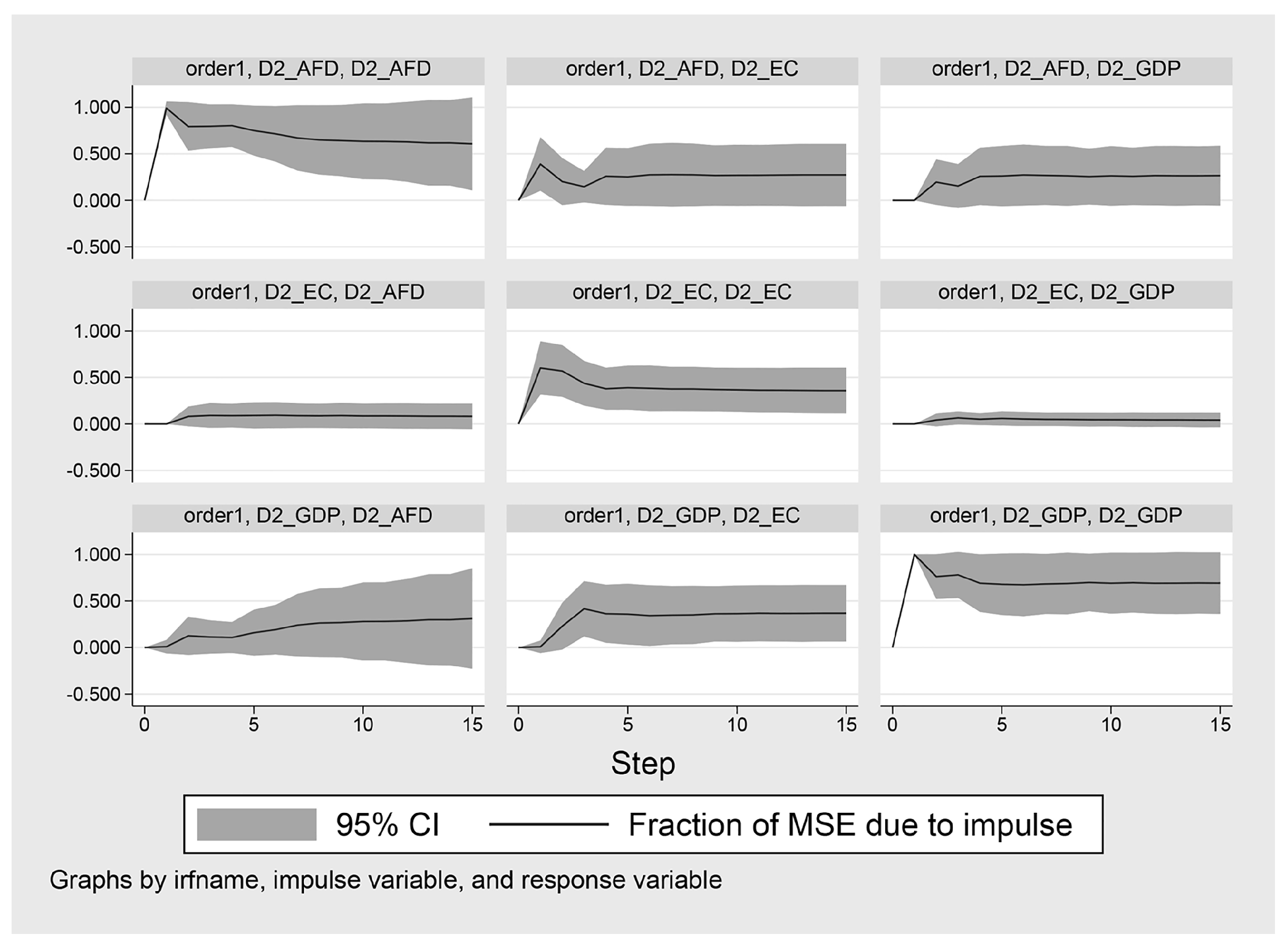
The results of the impulse response of Model 3 are shown in Figure 9, where agroforestry development (D2_AFD) is affected by a one-unit standard deviation shock to the VAR system: Agroforestry development (D2_AFD) absorbs the shock, decreases, and then increases by the corresponding percentage unit, and this effect subsides until after period 15. The impact of the shock on CO emissions (D2_CO) is absorbed instantaneously, decreases, and then increases, fluctuating cyclically until it plateaus after period 15. Energy consumption (D2_EC) is affected by this shock and absorbs it instantaneously, decreasing and then increasing, reaching a minimum peak in period 3 and then slowly decreasing and leveling off after period 15.
The impact on the VAR system of a shock to CO emissions (D2_CO) of one unit standard deviation is as follows: Agroforestry development (D2_AFD) absorbs the shock, rising and then falling, reaching a minimum peak in period 8, and gradually leveling off after period 10. After period 15, the effect slowly declines. Energy consumption (D2_EC) is affected by this shock and absorbs it instantaneously, rising and then falling, before declining and leveling off after period 10.
The impact on the VAR system of a one-unit standard deviation shock to energy consumption (D2_EC) is as follows: Agroforestry development (D2_AFD) absorbs the shock instantaneously, increases, and then decreases, and this effect subsides until after period 10. The effect will continue to rise and fluctuate until it subsides after period 10. Energy consumption (D2_EC) and CO emissions (D2_CO) show similar changes and increase by a corresponding percentage of units.
The results of the impulse response of Model 4 are shown in Figure 10, where CO emissions (D2_CO) are affected by a shock of one unit standard deviation to the VAR system: CO emissions (D2_CO) absorb the shock, first decreasing and then increasing by the corresponding percentage of units, and this effect subsides until after period 15. Energy consumption (D2_EC) is affected by this shock and absorbs it instantaneously, rising and then falling, peaking in period 3, before declining and leveling off in period 10. Population size (D2_PS) is affected by this shock and absorbs it instantaneously, rising and then falling, before leveling off after period 20.
The impact on the VAR system of a shock to energy consumption (D2_EC) of one unit standard deviation is as follows: CO emissions (D2_CO) absorb the shock instantaneously, falling and then rising, peaking in period 2, and leveling off after period 10. Energy consumption (D2_EC) is affected by this shock and absorbs it instantaneously, decreasing and then increasing, before declining after period 15. Population size (D2_PS) is affected by this shock and absorbs it instantly, decreasing and then increasing, before decreasing and leveling off after period 20.
The impact on the VAR system of a unit standard deviation shock to population size (D2_PS) is as follows: CO emissions (D2_CO) absorb the shock instantaneously, rising and then falling, gradually rising and peaking in period 9, and then leveling off after period 20. Energy consumption (D2_EC) is affected by this shock and absorbs it instantaneously, rising and then falling, and then continuing to fluctuate upwards until period 25. Population size (D2_PS) is affected by this shock and absorbs the shock until it falls, reaching a minimum peak in period 5, then rising and leveling off after period 10.
The results of the impulse response of Model 5 are shown in Figure 11, where agroforestry development (D2_AFD) is affected by a shock of one unit standard deviation to the VAR system: Agroforestry development (D2_AFD) absorbs the shock by first decreasing and then increasing by a corresponding percentage unit, and this effect remains until period 30. CO emissions (D2_CO) will absorb the shock instantaneously, decreasing and then increasing, and will continue to fluctuate, and this effect will not subside until period 30. Energy consumption (D2_EC) absorbs the shock, decreases, and then increases by a percentage of the corresponding unit, and this effect does not subside until period 30. Economic development (D2_GDP) is affected by this shock and absorbs it instantaneously, decreasing and then increasing, and this effect does not subside until period 30.
CO emissions (D2_CO) are affected by a shock of one unit standard deviation to the VAR system: Agroforestry development (D2_AFD) absorbs the shock instantaneously, rising and then falling, reaching a minimum peak in period 2, which subsides until period 10. The effect slowly declines after period 10. Energy consumption (D2_EC) is affected by this shock and absorbs it instantaneously, rising and then falling, before continuing to fluctuate upwards, with the effect slowly declining and leveling off after period 10. Economic development (D2_GDP) is affected by this shock and absorbs it instantaneously, decreasing and then increasing, and this effect remains in place until period 30.
The impact of a unit standard deviation shock to energy consumption (D2_EC) on the VAR system is as follows: Agroforestry development (D2_AFD) absorbs the shock instantaneously, decreasing and then increasing, and this effect subsides after period 10. The impact of the shock on CO emissions (D2_CO) is absorbed instantaneously, decreasing and then increasing, and gradually subsiding after period 10. Energy consumption (D2_EC) is affected by this shock and absorbs it, decreasing and then increasing, with the effect declining and leveling off after period 10. Economic development (D2_GDP) is affected by this shock and absorbs it instantaneously, decreasing and then increasing, and this effect remains in place until period 30.
The impact on the VAR system of a one-unit standard deviation shock to economic development (D2_GDP) is as follows: Agroforestry development (D2_AFD) absorbs the shock instantaneously, rising and then falling, and the impact remains unabated until period 30. CO emissions (D2_CO) absorb the shock instantaneously, falling and then rising, and the impact remains unabated until period 30. Energy consumption (D2_EC) is affected by this shock and absorbs the shock, rising and then falling, and this effect does not subside until period 30. Economic development (D2_GDP) is affected by this shock and absorbs it instantaneously, decreasing and then increasing.
4.5. Variance Decomposition
Analysis of the variance decomposition of the VAR model captures information on the relative importance of each stochastic disturbance term in the system that has an impact on the endogenous variables, the contribution of each structural shock to changes in the endogenous variables, and so on.
The results of the variance decomposition of Model 1 are shown in Figure 12. Agroforestry development (D2_AFD) has a positive shock effect on itself, reaching its strongest point in period 2, then gradually weakening, rising slightly in period 5, and then leveling off. Agroforestry development (D2_AFD) has a positive impact on energy consumption (D2_EC), which is strongest in period 2, rises slightly in period 5, and then plateaus. Agroforestry development (D2_AFD) exerts a positive shock on economic development (D2_GDP), which continues to be high, declines slightly in period 4, rises slightly in period 5, and then levels off.
Energy consumption (D2_EC) has a slight positive impact on agroforestry development (D2_AFD). Energy consumption (D2_EC) has a significant positive impact on itself, reaching its strongest point in period 2, then gradually decreasing and leveling off after period 5. Energy consumption (D2_EC) has a slight positive impact on economic development (D2_GDP), which is not significant.
Economic development (D2_GDP) has a significant positive impact on agroforestry development (D2_AFD) and shows a continuous trend of strength. Economic development (D2_GDP) has a significant positive shock effect on energy consumption (D2_EC), which reaches its strongest point in period 3, then decreases slightly, and finally plateaus. Economic development (D2_GDP) exerts a significant positive shock effect on itself, reaching its strongest point in period 2, then decreasing slightly, and leveling off after period 5.
The results of the variance decomposition of Model 2 are shown in Figure 13, where agroforestry development (D2_AFD) has a significant positive impact on itself, reaching its strongest point in period 2, and then slightly weakening and leveling off. Agroforestry development (D2_AFD) has a positive impact on energy consumption (D2_EC) and tends to increase gradually. Agroforestry development (D2_AFD) has a significant positive impact on population size (D2_PS), which tends to increase gradually.
Energy consumption (D2_EC) has a slight positive impact on agroforestry development (D2_AFD), but the impact is not significant. Energy consumption (D2_EC) has a significant positive impact on itself, reaching its strongest point in period 2, then decreasing and leveling off after period 5. Energy consumption (D2_EC) has a slight positive impact on population size (D2_PS), which is not significant. Population size (D2_PS) has a slight positive shock on agroforestry development (D2_AFD), which is insignificant. Population size (D2_PS) has a slight positive shock on energy consumption (D2_EC), which is insignificant. Population size (D2_PS) exerts a significant positive shock on itself, reaching its strongest point in period 2, then decreasing slightly and leveling off after period 5.
The results of the variance decomposition of Model 3 are shown in Figure 14, which shows that agroforestry development (D2_AFD) has a significant positive impact on itself, reaching its strongest point in period 2, and then slightly weakening and leveling off. Agroforestry development (D2_AFD) has a significant positive impact on CO emissions (D2_CO), which tend to increase gradually. Agroforestry development (D2_AFD) has a positive impact on energy consumption (D2_EC), which tends to increase gradually.
CO emissions (D2_CO) have a slight positive impact on agroforestry development (D2_AFD), but the impact is not significant. CO emissions (D2_CO) have a significant positive impact on themselves, reaching their strongest point in period 2, then gradually weakening and leveling off after period 5. CO emissions (D2_CO) have a slight positive impact on energy consumption (D2_EC), but the impact is not significant.
Energy consumption (D2_EC) has a slight positive impact on agroforestry development (D2_AFD), but the impact is not significant. Energy consumption (D2_EC) has a slight positive impact on CO emissions (D2_CO), but the impact is not significant. Energy consumption (D2_EC) exerts a significant positive shock on itself, reaching its strongest point in period 2, then decreasing slightly and leveling off after period 5.
The results of the variance decomposition of Model 4 are shown in Figure 15. CO emissions (D2_CO) have a significant positive shock effect on themselves, reaching their strongest point in period 2, then weakening slightly, and leveling off after period 5. CO emissions (D2_CO) have a positive impact on energy consumption (D2_EC), but the impact is not significant. CO emissions (D2_CO) have a positive impact on population size (D2_PS), which tends to increase gradually.
Energy consumption (D2_EC) has a significant positive impact on CO emissions (D2_CO), with an increasing trend. Energy consumption (D2_EC) has a significant positive impact on itself, reaching its strongest point in period 2, then decreasing slightly and leveling off after period 5. Energy consumption (D2_EC) has a slight positive impact on population size (D2_PS), which is not significant.
Population size (D2_PS) has a slight positive impact on CO emissions (D2_CO), but the impact is not significant. Population size (D2_PS) has a slight positive impact on energy consumption (D2_EC), but the impact is insignificant. Population size (D2_PS) has a significant positive impact on itself, reaching its strongest point in period 2, and then decreasing and leveling off.
The results of the variance decomposition of Model 5 are shown in Figure 16, which shows that agroforestry development (D2_AFD) has a significant positive impact on itself, reaching its strongest point in period 2, and then slightly weakening and leveling off. Agroforestry development (D2_AFD) has a significant positive impact on CO emissions (D2_CO), which tend to increase gradually. Agroforestry development (D2_AFD) has a significant positive impact on energy consumption (D2_EC), which is strongest in period 2, then weakens slightly, and levels off after period 5. Agroforestry development (D2_AFD) has a positive impact on economic development (D2_GDP) and tends to increase gradually.
CO emissions (D2_CO) have a slight positive impact on agroforestry development (D2_AFD), which tends to increase gradually. CO emissions (D2_CO) have a significant positive impact on themselves, reaching their strongest point in period 2, and then weakening slightly and leveling off. CO emissions (D2_CO) have a slight positive impact on energy consumption (D2_EC), which is insignificant. CO emissions (D2_CO) have almost no significant impact on economic development (D2_GDP).
Energy consumption (D2_EC) has a slight positive impact on agroforestry development (D2_AFD), but the impact is not significant. Energy consumption (D2_EC) has a positive impact on CO emissions (D2_CO), but the impact is not significant. Energy consumption (D2_EC) exerts a significant positive shock on itself, reaching its strongest point in period 2, then decreasing slightly and leveling off after period 5. Energy consumption (D2_EC) has almost no significant impact on economic development (D2_GDP).
Economic development (D2_GDP) has a significant positive impact on agroforestry development (D2_AFD), which continues to show a strong trend. Economic development (D2_GDP) has a significant positive impact on CO emissions (D2_CO), which continues to show a strong trend. Economic development (D2_GDP) has a significant positive impact on energy consumption (D2_EC) and shows a continuous strong trend. Economic development (D2_GDP) exerts a significant positive shock on itself, reaching its strongest point in period 2, then decreasing slightly and leveling off after period 5.
4.6. Forecast
The test results of several VAR models are shown in Table 6. From the test results in Table 6, it can be seen that the five VAR models fit well overall, with most of the p-values significant at the 1% level and only a few p-values significant at the 5% level.
The results of several different VAR models for agroforestry development (AFD) are shown in Figure 17. The overall trend shows that China’s AFD declines in 2021, then continues to rise in 2022 and 2023, declines slightly in 2024, and continues to rise in 2025.
The results of several different VAR models for energy consumption (EC) projections are shown in Figure 18. The overall trend shows a decrease in 2021, an increase in 2022, a slight decrease in 2023, a significant decrease in 2024, and a slight increase in 2025.
The results of several different VAR model projections for CO emissions (CO) are shown in Figure 19. The overall trend shows an increase in 2021, a slight decrease in 2022, a slight increase in 2023, a significant decrease in 2024, and an increase in 2025.
5. Discussion
5.1. Research Shortcomings
There are three main shortcomings in this paper: (1) There are many other factors that influence CO emissions, and in this paper we have only explored the impact of economic development, agricultural and forestry development, energy consumption, and population numbers on CO emissions. However, in reality, these factors may not be the main influencing factors, for example, there are also industrial production, power systems, and other production and operation activities that may emit more CO. (2) We have only studied 31 years of data, from 1990 to 2020, in China, and although we have selected 103 secondary indicators, we believe that this amount of data is far from sufficient. (3) Our study is only based on a linear relationship, but the effects of economic development, agroforestry development, energy consumption, and population size on CO emissions may be influenced by a non-linear relationship.
5.2. Future Perspectives
In the future, we will add more variables to study the factors influencing CO emissions in China, not only at the macro level to explore the relationships between them, but also at the micro level to investigate the causes of CO emissions in detail. In addition, we will collect as much indicator data as possible and increase the time span in order to add value and meaning to our research.
6. Conclusions and Implications
6.1. Conclusions
(1) There is a direct and significant positive relationship between economic development (GDP) and agroforestry development (AFD). There is an indirect relationship between economic development (GDP) and energy consumption (EC), with a significant positive effect. There is an indirect relationship between economic development (GDP) and energy consumption (PS), with a significant negative effect. There is both a direct and indirect effect between economic development (GDP) and carbon dioxide emissions (CO), with an overall significant positive effect.
Economic development provides the space and resource base for the development of agriculture and forestry. Energy is one of the essential factors of production, and although the intensity of energy consumption has been decreasing in recent years, the total consumption has been increasing. At the same time, the capital accumulation brought by economic development provides the basis for industrial development and production and manufacturing, leading to a new round of energy demand. Economic development reflects the level of social civilization and the demographic needs of social development, and therefore the demographic structure is constantly adjusting, with economic development determining the natural changes in population. Generally speaking, the higher the level of economic development, the lower the fertility level and the lower the birth and death rates of the population. Therefore, economic development can indirectly affect CO emissions through people’s basic carbon emissions; industrial, agricultural, and forestry production; and energy consumption. Economic development can also directly affect carbon dioxide emissions, which may be due to the accelerated circulation of capital, products, and factors due to good economic performance and more frequent economic activities, thus affecting the carbon emission performance of industries and enterprises.
Like economic development, agroforestry development is an important part of the economic system and exhibits the same impact relationships.
The relationship between agroforestry development (AFD) and energy consumption (EC) is direct and significantly positive. There is an indirect effect between AFD and population size (PS), which is significantly negative. There is both a direct and an indirect effect between AFD and CO emissions, with an overall significant positive effect.
The relationship between energy consumption (EC) and population size (PS) is direct and significantly negative. The relationship between energy consumption (EC) and carbon dioxide emissions (CO) is both direct and indirect, with an overall positive relationship. The relationship between population size (PS) and carbon dioxide emissions (CO) is direct and negative.
Fossil energy sources of all types are the main source of carbon; therefore, the use of energy to participate in combustion activities and industrial production and manufacturing increases CO emissions. The effect of energy consumption on population size may arise from the demographic restructuring due to economic growth. In contrast, the negative effect of population size on CO emissions may originate from the fact that the level of reduction of carbon emissions per capita is much higher than that caused by the growth of population size.
(2) The results of the Granger causality test show that economic development, energy consumption, and CO emissions are the causes of the constraints on agroforestry development. Economic development, agroforestry development, population size, and CO emissions are influences that constrain energy consumption. Energy consumption constrains economic development and CO emissions. Agroforestry development will affect the number of people and energy consumption.
(3) Over the next three years, China’s agroforestry development will be affected by the impulse response of economic development, energy consumption, and CO emissions, and will show a declining development trend. Over the next three years, China’s energy consumption will be influenced by the impulse response of economic development, agroforestry development, population size, and CO emissions, with a decreasing development trend followed by an increasing development trend. Over the next three years, China’s CO emissions will be influenced by the impulse response of energy consumption and agroforestry development factors, showing a downward and then upward development trend.
6.2. Suggestions
Here are three policy suggestions.
(1) The premise of improving the ecological protection system is to improve the ecological civilization system. We start with the following three suggestions: first, improve the assessment and evaluation system of economic and social development; second, delineate the ecological protection red line, and construct an accountability system; third, establish safety laws and regulations, to improve the ecological environmental protection management system. To establish a complete ecological civilization protection system, ecological civilization system construction needs to keep pace with the times, constantly improve, and be based on top-level design. In the continuous practice of exploration, one must keep pace with the times, constantly improving the ecological civilization protection system, which requires actively mobilizing the masses to participate, with everyone involved.
(2) To establish a unified national agricultural and forestry market, improve the construction of factors and resource markets; strengthen the quality of services and commodity markets; and unify rules, standards, and procedures for supervision. Local governments can combine local characteristics to introduce modern management, intensive production, and unified marketing and purchasing using a national unified market platform. Furthermore, the internal consumption of resources in small-scale production should be reduced, and more use should be made of technological innovation, industrial upgrading, and smooth national circulation of agricultural and forestry products.
(3) The Chinese government should increase financial subsidies for agriculture and forestry, and local governments should take into account the actual local situation; formulate guidelines and programs for the region; strengthen supervision, monitoring, and enforcement; and implement subsidies to encourage the agriculture and forestry industries to contribute to the reduction of CO emissions. At the same time, the government should vigorously develop new energy industries such as wind energy and solar energy to reduce the consumption of fossil energy; strengthen the integration of industry, academia, and research to promote the development of green low-carbon technology and clean energy technology; and strengthen publicity to cultivate civic awareness so that everyone can be a practitioner and advocate of low-carbon development.
6.3. Managerial Implications
(1) This paper constructs a more scientific and comprehensive indicator system from the perspective of asymmetric impact thinking, and empirically analyzes the relationship between economic development, agricultural and forestry development, population size, energy consumption, and the impact of CO emissions. This paper provides theoretical references and references for China’s economic development and the achievement of the carbon peak target under the epidemic.
(2) At a time when the global epidemic is raging, China’s economic development is also in the doldrums. At the same time, the Chinese government is faced with a dilemma between environmental protection and economic development. If the Chinese government continues to promote its “double carbon” strategy, economic development will inevitably suffer. Population decline is a foregone conclusion, consumption is weak, and fertility rates continue to weaken; population growth is the best option for boosting domestic demand. This shows that the level of quality economic development and green development in the country is still low. At the same time, as a large producer, high energy consumption promotes carbon emissions, which also indicates a low level of green production technologies. At present, China has undertaken carbon-neutral work in the areas of pilot construction and promotion of carbon sink markets, clean energy research and development, promotion of new energy vehicles, capacity reduction and differential tariffs, certification of “carbon-neutral enterprises”, technology, and financial subsidies. This paper argues that strengthening the development of agroforestry complex management, accelerating the modern management and upgrading of agroforestry complex management, and vigorously developing an agroforestry complex management economy is the best choice to balance economic development and environmental protection.
6.4. Social Implications
The international situation is volatile, and economic uncertainty has increased, affected by the COVID-19 epidemic and war. China’s aspirations to be carbon neutral by 2060 are even more daunting. To facilitate the acceleration of the carbon neutrality process, we have examined the impact of EC, AFD, EC, and PS on CO emissions. In order to better describe these elements in China, we have chosen as many variables as possible. There are two main points: (1) multiple variables make the trends of change more stable and help to avoid anomalous changes of variables; (2) the construction of EC, PS, and ADF will enrich the whole research framework. This is because it is in line with the current situation of the Chinese economy and the complexity of the economic system itself.
Author Contributions
Conceptualization, Q.L.; methodology, H.L.; software, H.L.; validation, all authors; formal analysis, H.L.; resources, Q.L.; data management, all authors; writing—original manuscript, H.L. and J.L.; writing—editing and revision, all authors; visualization, all authors. All authors have read and agreed to the published version of the manuscript.
Funding
National Social Science Foundation of China (21ZD081 and 21ZDA014).
Institutional Review Board Statement
Not applicable.
Informed Consent Statement
Not applicable.
Data Availability Statement
The data presented in this study are available on request from the corresponding author. The data are not publicly available due to the processing of data from different sources; some were retrieved through an extensive interview campaign, others were obtained from institutional databases, and some were from published literature.
Acknowledgments
School of Economics and Management, Nanjing Forestry University, provided some data support.
Conflicts of Interest
The authors declare no conflict of interest.
Appendix A

Table A1.
Assignment of indicator weights in PLS-PM model results.
| Level 1 Indicator | Indicator Name | Symbol | Weight |
|---|---|---|---|
| Economic Development | Domestic general government health expenditure (% of GDP) | X | 0.058601 |
| (GDP) | Manufacturing, value added (% of GDP) | X | −0.055852 |
| Market capitalization of listed domestic companies (% of GDP) | X | 0.045206 | |
| Research and development expenditure (% of GDP) | X | 0.059284 | |
| GDP per capita (current LCU) | X | 0.056813 | |
| GDP per capita, PPP (constant 2017 international $) | X | 0.058212 | |
| Industry (including construction), value added (% of GDP) | X | −0.028804 | |
| GDP per capita growth (annual %) | X | −0.022887 | |
| GDP per capita (current USD) | X | 0.056472 | |
| Foreign direct investment, net inflows (% of GDP) | X | −0.027652 | |
| GDP (current USD) | X | 0.056251 | |
| Gross national expenditure (% of GDP) | X | −0.000448 | |
| GDP (current LCU) | X | 0.056500 | |
| Trade (% of GDP) | X | 0.018994 | |
| Gross domestic savings (% of GDP) | X | 0.039865 | |
| GDP growth (annual %) | X | −0.028592 | |
| Broad money (% of GDP) | X | 0.059169 | |
| Merchandise trade (% of GDP) | X | −0.000515 | |
| Inflation, GDP deflator: linked series (annual %) | X | −0.028316 | |
| Services, value added (% of GDP) | X | 0.058527 | |
| General government final consumption expenditure (% of GDP) | X | 0.042862 | |
| Claims on central government, etc. (% GDP) | X | 0.049255 | |
| GDP per capita, PPP (current international $) | X | 0.058145 | |
| PPP conversion factor, GDP (LCU per international $) | X | 0.057993 | |
| GDP, PPP (current international $) | X | 0.057935 | |
| GDP deflator (base year varies by country) | X | 0.059344 | |
| Agroforestry Development | Agriculture, forestry, and fishing, value added (constant LCU) | X | 0.151855 |
| (AFD) | Agriculture, forestry, and fishing, value added (% of GDP) | X | −0.145671 |
| Agriculture, forestry, and fishing, value added (current USD) | X | 0.146749 | |
| Agriculture, forestry, and fishing, value added (annual % growth) | X | −0.031939 | |
| Agriculture, forestry, and fishing, value added per worker (constant 2015 USD) | X | 0.145551 | |
| Agriculture, forestry, and fishing, value added (current LCU) | X | 0.148642 | |
| Agriculture, forestry, and fishing, value added (constant 2015 USD) | X | 0.151895 | |
| Forest rents (% of GDP) | X | −0.131377 | |
| Total natural resources rents (% of GDP) | X | −0.045632 | |
| Energy consumption | Energy-related methane emissions (% of total) | X | 0.067541 |
| (EC) | Renewable energy consumption (% of total final energy consumption) | X | −0.065592 |
| Nitrous oxide emissions in energy sector (thousand metric tons of CO equivalent) | X | 0.064501 | |
| Energy imports, net (% of energy use) | X | 0.066981 | |
| Investment in energy with private participation (current USD) | X | −0.007817 | |
| Fossil fuel energy consumption (% of total) | X | 0.066547 | |
| Public private partnerships investment in energy (current USD) | X | −0.001304 | |
| Energy use (kg of oil equivalent per capita) | X | 0.066538 | |
| Adjusted savings: energy depletion (current USD) | X | 0.047159 | |
| Nitrous oxide emissions in energy sector (% of total) | X | −0.047572 | |
| Alternative and nuclear energy (% of total energy use) | X | 0.066999 | |
| Adjusted savings: energy depletion (% of GNI) | X | −0.026126 | |
| GDP per unit of energy use (PPP $ per kg of oil equivalent) | X | 0.068223 | |
| Combustible renewables and waste (% of total energy) | X | −0.067900 | |
| Methane emissions in energy sector (thousand metric tons of CO equivalent) | X | 0.066770 | |
| GDP per unit of energy use (constant 2017 PPP $ per kg of oil equivalent) | X | 0.067174 | |
| Energy intensity level of primary energy (MJ/$2011 PPP GDP) | X | −0.063757 | |
| Energy use (kg of oil equivalent) per $1,000 GDP (constant 2017 PPP) | X | −0.063351 | |
| Coal rents (% of GDP) | X | 0.014803 | |
| Mineral rents (% of GDP) | X | 0.009687 | |
| Natural gas rents (% of GDP) | X | 0.055533 | |
| Oil rents (% of GDP) | X | −0.049966 | |
| Population size | Population, female (% of total population) | X | 0.036775 |
| (PS) | Population ages 40–44, male (% of male population) | X | −0.048668 |
| Population ages 20–24, female (% of female population) | X | 0.053098 | |
| Population ages 0–14, male | X | 0.065278 | |
| Age dependency ratio (% of working-age population) | X | 0.060491 | |
| Population ages 20–24, male (% of male population) | X | 0.050611 | |
| Rural population | X | 0.066585 | |
| Age dependency ratio, old (% of working-age population) | X | −0.060103 | |
| Population ages 25–29, female (% of female population) | X | 0.045971 | |
| Population ages 0–14, total | X | 0.065667 | |
| Population, male (% of total population) | X | −0.036775 | |
| Population, total | X | −0.069061 | |
| Age dependency ratio, young (% of working-age population) | X | 0.067056 | |
| Population ages 0–14 (% of total population) | X | 0.067810 | |
| Population ages 15–64, total | X | −0.068139 | |
| Population ages 0–14, female | X | 0.065971 | |
| Urban population | X | −0.068701 | |
| Population ages 15–64, female (% of female population) | X | −0.058857 | |
| Population ages 30–34, female (% of female population) | X | 0.019239 | |
| Population ages 35–39, male (% of male population) | X | 0.003181 | |
| Population ages 30–34, male (% of male population) | X | 0.018523 | |
| Population ages 35–39, female (% of female population) | X | 0.002284 | |
| Population ages 10–14, female (% of female population) | X | 0.056126 | |
| CO emissions | CO emissions (kt) | X | 0.054550 |
| (CO) | CO emissions from liquid fuel consumption (% of total) | X | −0.037179 |
| CO emissions from electricity and heat production, total (% of total fuel combustion) | X | 0.047387 | |
| CO emissions (kg per 2017 PPP $ of GDP) | X | −0.051396 | |
| CO emissions from other sectors, excluding residential buildings and commercial and public services (% of total fuel combustion) | X | −0.049226 | |
| Nitrous oxide emissions (thousand metric tons of CO equivalent) | X | 0.055019 | |
| CO emissions from solid fuel consumption (% of total) | X | −0.039872 | |
| CO emissions from manufacturing industries and construction (% of total fuel combustion) | X | -0.027487 | |
| CO emissions from solid fuel consumption (kt) | X | 0.053315 | |
| Methane emissions (kt of CO equivalent) | X | 0.053228 | |
| CO emissions from liquid fuel consumption (kt) | X | 0.055332 | |
| Agricultural nitrous oxide emissions (thousand metric tons of CO equivalent) | X | 0.050109 | |
| CO emissions (metric tons per capita) | X | 0.054258 | |
| CO emissions from gaseous fuel consumption (% of total) | X | 0.050284 | |
| Agricultural methane emissions (thousand metric tons of CO equivalent) | X | −0.028583 | |
| CO emissions from gaseous fuel consumption (kt) | X | 0.052104 | |
| CO emissions (kg per 2015 USD of GDP) | X | −0.051440 | |
| Total greenhouse gas emissions (kt of CO equivalent) | X | 0.054590 | |
| CO emissions from residential buildings and commercial and public services (% of total fuel combustion) | X | −0.051083 | |
| CO emissions (kg per PPP $ of GDP) | X | −0.051347 | |
| CO emissions from transport (% of total fuel combustion) | X | 0.046346 | |
| Other greenhouse gas emissions, HFC, PFC and SF6 (thousand metric tons of CO equivalent) | X | −0.047617 | |
| CO intensity (kg per kg of oil equivalent energy use) | X | 0.051875 |
Table A2.
Results of Granger’s causality test.
| Model | Excluded | Equation | chi2 | df | Prob > chi2 | |
|---|---|---|---|---|---|---|
| Model 1 | AFD | → | GDP | 3.3493 | 2 | 0.1870 |
| EC | → | GDP | 7.1586 | 2 | 0.0280 ** | |
| ALL | → | GDP | 20.8700 | 4 | 0.0000 *** | |
| GDP | → | AFD | 7.0421 | 2 | 0.0300 ** | |
| EC | → | AFD | 8.5733 | 2 | 0.0140 ** | |
| ALL | → | AFD | 10.2840 | 4 | 0.0360 ** | |
| GDP | → | EC | 30.2920 | 2 | 0.0000 *** | |
| AFD | → | EC | 3.1659 | 2 | 0.2050 | |
| ALL | → | EC | 39.5070 | 4 | 0.0000 *** | |
| Model 2 | EC | → | AFD | 11.1580 | 5 | 0.0480 ** |
| PS | → | AFD | 4.9533 | 5 | 0.4220 | |
| ALL | → | AFD | 15.4730 | 10 | 0.1160 | |
| AFD | → | EC | 45.8530 | 5 | 0.0000 *** | |
| PS | → | EC | 9.6037 | 5 | 0.0870 * | |
| ALL | → | EC | 50.6000 | 10 | 0.0000 *** | |
| AFD | → | PS | 19.5970 | 5 | 0.0010 *** | |
| EC | → | PS | 6.3804 | 5 | 0.2710 | |
| ALL | → | PS | 20.1500 | 10 | 0.0280 ** | |
| Model 3 | EC | → | AFD | 11.1580 | 5 | 0.0480 ** |
| PS | → | AFD | 4.9533 | 5 | 0.4220 | |
| ALL | → | AFD | 15.4730 | 10 | 0.1160 | |
| AFD | → | EC | 45.8530 | 5 | 0.0000 *** | |
| PS | → | EC | 9.6037 | 5 | 0.0870 * | |
| ALL | → | EC | 50.6000 | 10 | 0.0000 *** | |
| AFD | → | PS | 19.5970 | 5 | 0.0010 *** | |
| EC | → | PS | 6.3804 | 5 | 0.2710 | |
| ALL | → | PS | 20.1500 | 10 | 0.0280 ** | |
| Model 4 | PS | → | EC | 14.1000 | 5 | 0.0150 ** |
| CO | → | EC | 36.0450 | 5 | 0.0000 *** | |
| ALL | → | EC | 40.1260 | 10 | 0.0000 *** | |
| EC | → | PS | 2.0216 | 5 | 0.8460 | |
| CO | → | PS | 3.2389 | 5 | 0.6630 | |
| ALL | → | PS | 3.5842 | 10 | 0.9640 | |
| EC | → | CO | 31.1310 | 5 | 0.0000 *** | |
| PS | → | CO | 6.5185 | 5 | 0.2590 | |
| ALL | → | CO | 39.4350 | 10 | 0.0000 *** | |
| Model 5 | AFD | → | GDP | 4.8862 | 2 | 0.0870 * |
| EC | → | GDP | 5.8958 | 2 | 0.0520 * | |
| CO | → | GDP | 2.4567 | 2 | 0.2930 | |
| ALL | → | GDP | 25.2260 | 6 | 0.0000 *** | |
| GDP | → | AFD | 6.3174 | 2 | 0.0420 ** | |
| EC | → | AFD | 15.5890 | 2 | 0.0000 *** | |
| CO | → | AFD | 15.1700 | 2 | 0.0010 *** | |
| ALL | → | AFD | 31.2320 | 6 | 0.0000 *** | |
| GDP | → | EC | 20.7500 | 2 | 0.0000 *** | |
| AFD | → | EC | 1.8891 | 2 | 0.3890 | |
| CO | → | EC | 1.1055 | 2 | 0.5750 | |
| ALL | → | EC | 42.2300 | 6 | 0.0000 *** | |
| GDP | → | CO | 0.1936 | 2 | 0.9080 | |
| AFD | → | CO | 1.9974 | 2 | 0.3680 | |
| EC | → | CO | 4.4610 | 2 | 0.1070 | |
| ALL | → | CO | 14.7870 | 6 | 0.0220 ** |
*** indicates significance at the 1% level. ** indicates significance at the 5% level. * indicates significance at the 10% level. Similarly hereinafter
References
- Murshed, M.; Alam, M.S. An estimation of the macroeconomic determinants total, renewable and non-renewable energy demands in Bangladesh: The role of technological innovations. Environ. Sci. Pollut. Control Ser. 2021, 28, 30176–30196. [Google Scholar] [CrossRef] [PubMed]
- Zeng, Y.; Maxwell, S.; Runting, R.K.; Venter, O.; Watson, J.E.; Carrasco, L.R. Environmental destruction not avoided with the sustainable development goals. Nat. Sustain. 2020, 3, 795–798. [Google Scholar] [CrossRef]
- Murshed, M. Can regional trade integration facilitate renewable energy transition to ensure energy sustainability in South Asia? Energy Rep. 2021, 7, 808–821. [Google Scholar] [CrossRef]
- Jacobson, M.Z. Review of solutions to global warming, air pollution, and energy security. Energy Environ. Sci. 2009, 2, 148–173. [Google Scholar] [CrossRef]
- Ghodake, G.S.; Shinde, S.K.; Kadam, A.A.; Saratale, R.G.; Saratale, G.D.; Kumar, M.; Kim, D.Y. Review on biomass feedstocks, pyrolysis mechanism and physicochemical properties of biochar: State-of-the-art framework to speed up vision of circular bioeconomy. J. Clean. Prod. 2021, 297, 126645. [Google Scholar] [CrossRef]
- FAO. Tracking Progress on Food and Agriculture-Related SDG Indicators 2021. 2021. Available online: https://www.fao.org/sdg-progress-report/en/ (accessed on 26 April 2022).
- Liu, H.; Fan, L.; Shao, Z. Threshold effects of energy consumption, technological innovation, and supply chain management on enterprise performance in China’s manufacturing industry. J. Environ. Manag. 2021, 300, 113687. [Google Scholar] [CrossRef]
- Sha, T.; Li, Q.; Yu, F.W. Blue Book of Low-Carbon Development: Annual Report on the Carbon Neutrality in China; Social Sciences Academic Press (China): Beijing, China, 2022. [Google Scholar]
- Ding, C.; Liu, C.; Zheng, C.; Li, F. Digital Economy, Technological Innovation and High-Quality Economic Development: Based on Spatial Effect and Mediation Effect. Sustainability 2022, 14, 216. [Google Scholar] [CrossRef]
- Lu, C.; Wang, D.; Li, H.; Cheng, W.; Tang, X.; Liu, W. Measurement of the Degree of Coordination in Regard to Carbon Emissions, Economic Development, and Environmental Protection in China. Appl. Sci. 2021, 11, 1750. [Google Scholar] [CrossRef]
- Shi, H.; Chai, J.; Lu, Q.; Zheng, J.; Wang, S. The impact of China’s low-carbon transition on economy, society and energy in 2030 based on CO2 emissions drivers. Energy 2022, 239, 122336. [Google Scholar] [CrossRef]
- Pervaiz, R.; Faisal, F.; Rahman, S.U.; Chander, R.; Ali, A. Do health expenditure and human development index matter in the carbon emission function for ensuring sustainable development? Evidence from the heterogeneous panel. Air Qual. Atmos. Health 2021, 14, 1773–1784. [Google Scholar] [CrossRef]
- Wu, R.; Ma, T.; Schrder, E. The contribution of trade to production-Based carbon dioxide emissions. Struct. Chang. Econ. Dyn. 2022, 60, 391–406. [Google Scholar] [CrossRef]
- Sharma, M.; Kaushal, R.; Kaushik, P.; Ramakrishna, S. Carbon Farming: Prospects and Challenges. Sustainability 2021, 13, 11122. [Google Scholar] [CrossRef]
- Platis, D.P.; Anagnostopoulos, C.D.; Tsaboula, A.D.; Menexes, G.C.; Kalburtji, K.L.; Mamolos, A.P. Energy Analysis, and Carbon and Water Footprint for Environmentally Friendly Farming Practices in Agroecosystems and Agroforestry. Sustainability 2019, 11, 1664. [Google Scholar] [CrossRef] [Green Version]
- Association for Temperate Agroforestry(AFTA). What Is Agroforestry? 2021. Available online: https://www.aftaweb.org/about/what-is-agroforestry.html (accessed on 26 April 2022).
- Bishaw, B.; Soolanayakanahally, R.; Karki, U.; Hagan, E. Agroforestry for sustainable production and resilient landscapes. Agrofor. Syst. 2022, 96, 447–451. [Google Scholar] [CrossRef]
- Ji, S.; Lee, Y. Food security and agroforestry from the perspective of the SDGs: A case study of the Democratic People’s Republic of Korea. Int. For. Rev. 2021, 23, 437–447. [Google Scholar] [CrossRef]
- Ma, S.; Qiao, Y.P.; Wang, L.J.; Zhang, J.C. Terrain gradient variations in ecosystem services of different vegetation types in mountainous regions: Vegetation resource conservation and sustainable development. For. Ecol. Manag. 2021, 482, 118856. [Google Scholar] [CrossRef]
- Callo-Concha, D.; Denich, M.; Ul Hassan, M.M.; Place, F.; Wardell, D.A. Lessons for research, capacity development and policy in agroforestry for development. Agrofor. Syst. 2017, 91, 795–798. [Google Scholar] [CrossRef]
- Tschora, H.; Cherubini, F. Co-benefits and trade-offs of agroforestry for climate change mitigation and other sustainability goals in West Africa. Glob. Ecol. Conserv. 2020, 22, e00919. [Google Scholar] [CrossRef]
- Lojka, B.; Teutscherová, N.; Chládová, A.; Kala, L.; Szabó, P.; Martiník, A.; Lawson, G. Agroforestry in the Czech Republic: What hampers the comeback of a once traditional land use system? Agronomy 2021, 12, 69. [Google Scholar] [CrossRef]
- Udawatta, R.P.; Rankoth, L.M.; Jose, S. Agroforestry and biodiversity. Sustainability 2019, 11, 2879. [Google Scholar] [CrossRef] [Green Version]
- Guimarães, N.; Pádua, L.; Marques, P.; Silva, N.; Peres, E.; Sousa, J.J. Forestry remote sensing from unmanned aerial vehicles: A review focusing on the data, processing and potentialities. Remote. Sens. 2020, 12, 1046. [Google Scholar] [CrossRef] [Green Version]
- Schier, H.E.; Eliot, K.A.; Herron, S.A.; Landfried, L.K.; Migicovsky, Z.; Rubin, M.J.; Miller, A.J. Comparative analysis of perennial and annual Phaseolus seed nutrient concentrations. Sustainability 2019, 11, 2787. [Google Scholar] [CrossRef] [Green Version]
- Lowry, G.V.; Avellan, A.; Gilbertson, L.M. Opportunities and challenges for nanotechnology in the agri-tech revolution. Nat. Nanotechnol. 2019, 14, 517–522. [Google Scholar] [CrossRef]
- Leeson, G.W. The growth, ageing and urbanisation of our world. J. Popul. Ageing 2018, 11, 107–115. [Google Scholar] [CrossRef] [Green Version]
- United Nations. World Population Prospects: 2017 Revision; Department of Economic and Social Affairs: New York, NY, USA, 2017; Available online: https://www.un.org/development/desa/publications/world-population-prospects-the-2017-revision.html (accessed on 6 May 2022).
- Karthikeyan, L.; Chawla, I.; Mishra, A.K. A review of remote sensing applications in agriculture for food security: Crop growth and yield, irrigation, and crop losses. J. Hydrol. 2020, 586, 124905. [Google Scholar] [CrossRef]
- Rehman, A.; Ulucak, R.; Murshed, M.; Ma, H.; Işık, C. Carbonization and atmospheric pollution in China: The asymmetric impacts of forests, livestock production, and economic progress on CO2 emissions. J. Environ. Manag. 2021, 294, 113059. [Google Scholar] [CrossRef]
- Weiss, M.; Jacob, F.; Duveiller, G. Remote sensing for agricultural applications: A meta-review. Remote. Sens. Environ. 2020, 236, 111402. [Google Scholar] [CrossRef]
- Weselek, A.; Ehmann, A.; Zikeli, S.; Lewandowski, I.; Schindele, S.; Högy, P. Agrophotovoltaic systems: Applications, challenges, and opportunities. A review. Agron. Sustain. Dev. 2019, 39, 35. [Google Scholar] [CrossRef]
- Liu, X.; Zhang, S.; Bae, J. The impact of renewable energy and agriculture on carbon dioxide emissions: Investigating the environmental Kuznets curve in four selected ASEAN countries. J. Clean. Prod. 2017, 164, 1239–1247. [Google Scholar] [CrossRef]
- Qiao, H.; Zheng, F.; Jiang, H.; Dong, K. The greenhouse effect of the agriculture-economic growth-renewable energy nexus: Evidence from G20 countries. Sci. Total. Environ. 2019, 671, 722–731. [Google Scholar] [CrossRef]
- Qi, M.; Xu, J.; Amuji, N.B.; Wang, S.; Xu, F.; Zhou, H. The Nexus among Energy Consumption, Economic Growth and Trade Openness: Evidence from West Africa. Sustainability 2022, 14, 3630. [Google Scholar] [CrossRef]
- Kongkuah, M.; Yao, H.; Yilanci, V. The relationship between energy consumption, economic growth, and CO2 emissions in China: The role of urbanisation and international trade. Environ Dev. Sustain. 2022, 24, 4684–4708. [Google Scholar] [CrossRef]
- Azam, A.; Rafiq, M.; Shafique, M.; Zhang, H.; Ateeq, M.; Yuan, J. Analyzing the relationship between economic growth and electricity consumption from renewable and non-renewable sources: Fresh evidence from newly industrialized countries. Sustain. Energy Technol. Assess. 2021, 44, 100991. [Google Scholar] [CrossRef]
- Huisingh, D.; Zhang, Z.; Moore, J.C.; Qiao, Q.; Li, Q. Recent advances in carbon emissions reduction: Policies, technologies, monitoring, assessment and modeling. J. Clean. Prod. 2015, 103, 1–12. [Google Scholar] [CrossRef]
- Sane, M.; Hajek, M.; Phiri, J.; Babangida, J.S.; Nwaogu, C. Application of Decoupling Approach to Evaluate Electricity Consumption, Agriculture, GDP, Crude Oil Production, and CO2 Emission Nexus in Support of Economic Instrument in Nigeria. Sustainability 2022, 14, 3226. [Google Scholar] [CrossRef]
- Li, P.; Lang, M.; Zhu, S.; Bork, E.W.; Carlyle, C.N.; Chang, S.X. Greenhouse gas emissions are affected by land use type in two agroforestry systems: Results from an incubation experiment. Ecol. Res. 2020, 35, 1073–1086. [Google Scholar] [CrossRef]
- Bolson, N.; Yutkin, M.; Patzek, T. Energy efficiency and sustainability assessment for methane harvesting from Lake Kivu. Energy 2021, 225, 120215. [Google Scholar] [CrossRef]
- Chavan, S.B.; Newaj, R.; Rizvi, R.H.; Prasad, R.; Alam, B.; Handa, A.K.; Tripathi, D. Reduction of global warming potential vis-à-vis greenhouse gases through traditional agroforestry systems in Rajasthan, India. Environ. Dev. Sustain. 2021, 23, 4573–4593. [Google Scholar] [CrossRef]
- Keerthika, A.; Chavan, S.B.; Shukla, M. Khejri agroforestry for addressing issues of soil health. Life Sci. Leafl. 2015, 64, 102–108. [Google Scholar]
- Chavan, S.; Newaj, R.; Keerthika, A.; Ram, A.; Jha, A.; Kumar, A. Agroforestry for adaptation and mitigation of climate change. Pop. Kheti 2014, 4, 214–220. [Google Scholar]
- Raheem, A.; Prinsen, P.; Vuppaladadiyam, A.K.; Zhao, M.; Luque, R. A review on sustainable microalgae based biofuel and bioenergy production: Recent developments. J. Clean. Prod. 2018, 181, 42–59. [Google Scholar] [CrossRef]
- He, G.; Wang, K.; Zhong, Q.; Zhang, G.; van den Bosch, C.K.; Wang, J. Agroforestry reclamations decreased the CO2 budget of a coastal wetland in the Yangtze estuary. Agric. For. Meteorol. 2021, 296, 108212. [Google Scholar] [CrossRef]
- Brown, S.E.; Miller, D.C.; Ordonez, P.J.; Baylis, K. Evidence for the impacts of agroforestry on agricultural productivity, ecosystem services, and human well-being in high-income countries: A systematic map protocol. Environ. Evid. 2018, 7, 24. [Google Scholar] [CrossRef] [Green Version]
- Giannitsopoulos, M.L.; Graves, A.R.; Burgess, P.J.; Crous-Duran, J.; Moreno, G.; Herzog, F.; de Jalón, S.G. Whole system valuation of arable, agroforestry and tree-only systems at three case study sites in Europe. J. Clean. Prod. 2020, 269, 122283. [Google Scholar] [CrossRef]
- Xiang, H.; Yang, J.; Liu, X.; Lee, J. Balancing Population Distribution and Sustainable Economic Development in Yangtze River Economic Belt of China. Sustainability 2019, 11, 3320. [Google Scholar] [CrossRef] [Green Version]
- Sadorsky, P. Energy Related CO2 Emissions before and after the Financial Crisis. Sustainability 2020, 12, 3867. [Google Scholar] [CrossRef]
- Schaffer, C.; Eksvärd, K.; Björklund, J. Can agroforestry grow beyond its niche and contribute to a transition towards sustainable agriculture in Sweden? Sustainability 2019, 11, 3522. [Google Scholar] [CrossRef] [Green Version]
- Luo, X.; Xiong, K.; Zhang, J.; Chen, D. A Study on Optimal Agroforestry Planting Patterns in the Buffer Zone of World Natural Heritage Sites. Sustainability 2021, 13, 11544. [Google Scholar] [CrossRef]
- Cuéllar, M.A.; Allaire, S.E.; Lange, S.F.; Bradley, R.; Parsons, W.F.J.; Rivest, D.; Cogliastro, A. Greenhouse gas dynamics in agroforestry using tree based intercropping system under organic production. Can. J. Soil Sci. 2017, 97, 382–393. [Google Scholar]
- Hotelier-Rous, N.; Laroche, G.; Durocher, È.; Rivest, D.; Olivier, A.; Liagre, F.; Cogliastro, A. Temperate Agroforestry Development: The Case of Québec and of France. Sustainability 2020, 12, 7227. [Google Scholar] [CrossRef]
- Hirano, Y.; Ihara, T.; Hara, M.; Honjo, K. Estimation of Direct and Indirect Household CO2 Emissions in 49 Japanese Cities with Consideration of Regional Conditions. Sustainability 2020, 12, 4678. [Google Scholar] [CrossRef]
- Azam, A.; Rafiq, M.; Shafique, M.; Yuan, J. An empirical analysis of the non-linear effects of natural gas, nuclear energy, renewable energy and ICT-Trade in leading CO2 emitter countries: Policy towards CO2 mitigation and economic sustainability. J. Environ. Manag. 2021, 286, 112232. [Google Scholar] [CrossRef] [PubMed]
- Jung, T.Y.; Kim, Y.-G.; Moon, J. The Impact of Demographic Changes onCO2 Emission Profiles: Cases of East Asian Countries. Sustainability 2021, 13, 677. [Google Scholar] [CrossRef]
- Wang, H.; Zeng, W. Revealing Urban Carbon Dioxide (CO2) Emission Characteristics and Influencing Mechanisms from the Perspective of Commuting. Sustainability 2019, 11, 385. [Google Scholar] [CrossRef] [Green Version]
- Sun, X.; Wilmot, C.; Kasturi, T. Household travel, household characteristics, and land use: An empirical study from the 1994 Portland activity-based travel survey. Transp. Res. Rec. 1998, 1617, 10–17. [Google Scholar] [CrossRef]
- Zhu, H.; Pan, K.; Liu, Y.; Chang, Z.; Jiang, P.; Li, Y. Analyzing Temporal and Spatial Characteristics and Determinant Factors of Energy-Related CO2 Emissions of Shanghai in China Using High-Resolution Gridded Data. Sustainability 2019, 11, 4766. [Google Scholar] [CrossRef] [Green Version]
- Yang, Y.; Jia, J.; Chen, C. Residential Energy-Related CO2 Emissions in China’s Less Developed Regions: A Case Study of Jiangxi. Sustainability 2020, 12, 2000. [Google Scholar] [CrossRef] [Green Version]
- Pan, C.; Wang, H.; Guo, H.; Pan, H. How Do the Population Structure Changes of China Affect Carbon Emissions? An Empirical Study Based on Ridge Regression Analysis. Sustainability 2021, 13, 3319. [Google Scholar] [CrossRef]
- Guo, W.; Sun, T.; Dai, H. Effect of Population Structure Change on Carbon Emission in China. Sustainability 2016, 8, 225. [Google Scholar] [CrossRef] [Green Version]
- Zou, X.; Wang, R.; Hu, G.; Rong, Z.; Li, J. CO2 Emissions Forecast and Emissions Peak Analysis in Shanxi Province, China: An Application of the LEAP Model. Sustainability 2022, 14, 637. [Google Scholar] [CrossRef]
- Kassem, M.A. Risk Management Assessment in Oil and Gas Construction Projects Using Structural Equation Modeling (PLS-SEM). Gases 2022, 2, 33–60. [Google Scholar] [CrossRef]
- Hair, J.F.J.; Hult, G.T.M.; Ringle, C.; Sarstedt, M. A Primer on Partial Least Squares Structural Equation Modeling (PLS-SEM); Elsevier: Amsterdam, The Netherlands, 2014; Volume 46, pp. 184–185. [Google Scholar] [CrossRef]
- Hair, J.F.; Risher, J.J.; Sarstedt, M.; Ringle, C.M. When to use and how to report the results of PLS-SEM. Eur. Bus. Rev. 2019, 31, 2–24. [Google Scholar] [CrossRef]
- Sims, C.A. Comparison of interwar and postwar business cycles: Monetarism reconsidered. Am. Econ. Rev. 1980, 70, 250–257. [Google Scholar]
- Sims, C.A. Policy analysis with econometric models. Brookings Pap. Econ. Act. 1982, 1, 107–152. [Google Scholar] [CrossRef] [Green Version]
Figure 1.
Structure of the PLS-PM model.

Figure 2.
Unit circle test of model 1.

Figure 3.
Unit circle test of model 2.

Figure 4.
Unit circle test of model 3.

Figure 5.
Unit circle Test of model 4.

Figure 6.
Unit circle test of model 5.

Figure 7.
Impulse response of model 1.

Figure 8.
Impulse response of model 2.

Figure 9.
Impulse response of model 3.

Figure 10.
Impulse response of model 4.

Figure 11.
Impulse response of model 5.

Figure 12.
Variance decomposition of model 1.

Figure 13.
Variance decomposition of model 2.

Figure 14.
Variance decomposition of model 3.

Figure 15.
Variance decomposition of model 4.

Figure 16.
Variance decomposition of Model 5.

Figure 17.
AFD predicted by different models.

Figure 18.
EC predicted by different models.

Figure 19.
CO predicted by different models.

Table 1.
Descriptive analysis of variables.
| Variable | Year | GDP | AFD | EC | PS | CO |
|---|---|---|---|---|---|---|
| Obs | 31 | 31 | 31 | 31 | 31 | 31 |
| Mean | 2005 | 2710 × 10 | 1250 × 10 | 3100 × 10 | −1050 × 10 | 1,150,694 |
| Std. dev. | 9.092121 | 2510 × 10 | 631 × 10 | 2950 × 10 | 341 × 10 | 524,396.7 |
| Min | 1990 | 191 × 10 | 477 × 10 | 284 × 10 | −1560 × 10 | 484,923.7 |
| Max | 2020 | 8000 × 10 | 2520 × 10 | 11,100 × 10 | −517 × 10 | 1,869,574 |
Table 2.
PLS-PM model variable correlations and model goodness-of-fit.
| Variables | GDP | AFD | EC | PS | CO |
|---|---|---|---|---|---|
| GDP | 1.00 | 0.99 | 0.95 | −0.90 | 0.96 |
| AFD | 0.99 | 1.00 | 0.97 | −0.92 | 0.98 |
| EC | 0.95 | 0.97 | 1.00 | −0.98 | 0.99 |
| PS | −0.90 | −0.92 | −0.98 | 1.00 | −0.96 |
| CO | 0.96 | 0.98 | 0.99 | −0.96 | 1.00 |
| Estimate | −0.31 *** | 0.77 *** | 0.37 ** | −0.16 * | |
| Std. Error | 0.09 | 0.14 | 0.14 | 0.08 | |
| t value | −3.30 | 5.26 | 2.57 | −1.96 | |
| Pr(>|t|) | 0.00 | 0.00 | 0.01 | 0.06 | |
| R | 0.00 | 0.98 | 0.94 | 0.96 | 0.99 |
| Type | Exogenous | Endogenous | Endogenous | Endogenous | Endogenous |
*** indicates significance at the 1% level. ** indicates significance at the 5% level. * indicates significance at the 10% level. Similarly hereinafter.
Table 3.
Influence relationships between variables in PLS-PM model results.
| Relationships | Direct | Indirect | Total | |
|---|---|---|---|---|
| 1 | GDP ->AFD | 0.9900 | 0.0000 | 0.9900 |
| 2 | GDP ->EC | 0.0000 | 0.9630 | 0.9630 |
| 3 | GDP ->PS | 0.0000 | −0.9440 | −0.9440 |
| 4 | GDP ->CO | −0.3160 | 1.2880 | 0.9720 |
| 5 | AFD ->EC | 0.9730 | 0.0000 | 0.9730 |
| 6 | AFD ->PS | 0.0000 | −0.9540 | −0.9540 |
| 7 | AFD ->CO | 0.7740 | 0.5280 | 1.3010 |
| 8 | EC ->PS | −0.9800 | 0.0000 | −0.9800 |
| 9 | EC ->CO | 0.3790 | 0.1630 | 0.5420 |
| 10 | PS ->CO | −0.1670 | 0.0000 | −0.1670 |
Table 4.
ADF unit root test.
| Variables | Z (t) | p-Value | Differential Orders | Total |
|---|---|---|---|---|
| GDP | −5.5470 | 0.0000 | 2 | 0.9900 |
| AFD | −6.2300 | 0.0000 | 2 | 0.9630 |
| EC | −9.3190 | 0.0000 | 2 | −0.9440 |
| PS | −4.5030 | 0.0002 | 2 | 0.9720 |
| CO | −5.8980 | 0.0000 | 2 | 0.9730 |
| 6 | AFD → PS | 0.0000 | −0.9540 | −0.9540 |
| 7 | AFD → CO | 0.7740 | 0.5280 | 1.3010 |
| 8 | EC → PS | −0.9800 | 0.0000 | −0.9800 |
| 9 | EC → CO | 0.3790 | 0.1630 | 0.5420 |
| 10 | PS → CO | −0.1670 | 0.0000 | −0.1670 |
Table 5.
Johansen co-integration test.
| Max Rank | Params | LL | Eigenvalue | Trace Statistic | Critical Value 5% | |
|---|---|---|---|---|---|---|
| Model 1 | 0 | 12 | 51.10112 | 98.61640 | 29.68000 | |
| 1 | 17 | 85.40572 | 0.92122 | 30.00720 | 15.41000 | |
| 2 | 20 | 95.24057 | 0.51737 | 10.33750 | 3.76000 | |
| 3 | 21 | 100.40931 | 0.31810 | |||
| Model 2 | 0 | 39 | 100.52055 | 52.10080 | 29.68000 | |
| 1 | 44 | 114.71232 | 0.69353 | 23.71730 | 15.41000 | |
| 2 | 47 | 123.93795 | 0.53643 | 5.26600 | 3.76000 | |
| 3 | 48 | 126.57095 | 0.19701 | |||
| Model 3 | 0 | 30 | 68.16102 | 32.66860 | 29.68000 | |
| 1 | 35 | 76.24761 | 0.47635 | 16.49540 | 15.41000 | |
| 2 | 38 | 81.36629 | 0.33601 | 6.25810 | 3.76000 | |
| 3 | 39 | 84.49533 | 0.22145 | |||
| Model 4 | 0 | 39 | 89.56117 | 41.90160 | 29.68000 | |
| 1 | 44 | 101.54564 | 0.63164 | 17.93270 | 15.41000 | |
| 2 | 47 | 106.69543 | 0.34894 | 7.63310 | 3.76000 | |
| 3 | 48 | 110.51198 | 0.27243 | |||
| Model 5 | 0 | 20 | 94.52384 | 120.47980 | 47.21000 | |
| 1 | 27 | 128.77648 | 0.92091 | 51.97450 | 29.68000 | |
| 2 | 32 | 145.66508 | 0.71378 | 18.19730 | 15.41000 | |
| 3 | 35 | 151.58932 | 0.35521 | 6.34890 | 3.76000 | |
| 4 | 36 | 154.76375 | 0.20954 |
Table 6.
Test Results of five VAR models.
| Model | Equation | Parms | RMSE | R-sq | chi2 | p > chi2 |
|---|---|---|---|---|---|---|
| Model 1 | D2_GDP | 7 | 0.0295 | 0.6365 | 47.2757 | 0.0000 *** |
| D2_AFD | 7 | 0.0466 | 0.3736 | 16.1022 | 0.0132 ** | |
| D2_EC | 7 | 0.5078 | 0.8307 | 132.4766 | 0.0000 *** | |
| Model 2 | D2_AFD | 16 | 0.0594 | 0.5832 | 33.5843 | 0.0039 *** |
| D2_EC | 16 | 0.6872 | 0.8760 | 169.5574 | 0.0000 *** | |
| D2_PS | 16 | 0.0116 | 0.7241 | 62.9938 | 0.0000 *** | |
| Model 3 | D2_AFD | 13 | 0.0473 | 0.6066 | 38.5426 | 0.0001 *** |
| D2_EC | 13 | 0.5621 | 0.8756 | 175.8880 | 0.0000 *** | |
| D2_CO | 13 | 0.0594 | 0.6530 | 47.0547 | 0.0000 *** | |
| Model 4 | D2_EC | 16 | 0.7412 | 0.8558 | 142.3793 | 0.0000 *** |
| D2_PS | 16 | 0.0146 | 0.5584 | 30.3524 | 0.0107 ** | |
| D2_CO | 16 | 0.0703 | 0.6566 | 45.8892 | 0.0001 *** | |
| Model 5 | D2_GDP | 9 | 0.0298 | 0.6668 | 54.0341 | 0.0000 *** |
| D2_AFD | 9 | 0.0393 | 0.5989 | 40.3189 | 0.0000 *** | |
| D2_EC | 9 | 0.5247 | 0.8374 | 139.0061 | 0.0000 *** | |
| D2_CO | 9 | 0.0664 | 0.3696 | 15.8298 | 0.0449 ** |
*** indicates significance at the 1% level. ** indicates significance at the 5% level.
Publisher’s Note: MDPI stays neutral with regard to jurisdictional claims in published maps and institutional affiliations. |
© 2022 by the authors. Licensee MDPI, Basel, Switzerland. This article is an open access article distributed under the terms and conditions of the Creative Commons Attribution (CC BY) license (https://creativecommons.org/licenses/by/4.0/).
Share and Cite
MDPI and ACS Style
Liu, H.; Liu, J.; Li, Q. Asymmetric Effects of Economic Development, Agroforestry Development, Energy Consumption, and Population Size on CO2 Emissions in China. Sustainability 2022, 14, 7144. https://doi.org/10.3390/su14127144
AMA Style
Liu H, Liu J, Li Q. Asymmetric Effects of Economic Development, Agroforestry Development, Energy Consumption, and Population Size on CO2 Emissions in China. Sustainability. 2022; 14(12):7144. https://doi.org/10.3390/su14127144
Chicago/Turabian StyleLiu, Hui, Jiwei Liu, and Qun Li. 2022. "Asymmetric Effects of Economic Development, Agroforestry Development, Energy Consumption, and Population Size on CO2 Emissions in China" Sustainability 14, no. 12: 7144. https://doi.org/10.3390/su14127144
Note that from the first issue of 2016, this journal uses article numbers instead of page numbers. See further details here.