Resilience Enhancement of an Urban Microgrid during Off-Grid Mode Operation Using Critical Load Indicators

Abstract

Microgrids (MGs) can be used as a solution to ensure resilience against power supply failures in electricity grids caused by extreme weather conditions, unavailability of generation capacities, and problems with transmission components. The literature is rich in research focusing on strengthening the planning of microgrids based on overall load demand. In this study, a critical load demand indicator will be calculated and used to identify optimum operation strategies of microgrids in a power failure mode. An urban microgrid with a large educational building is selected for the case study. Operation dispatch scenarios are developed to reinforce the system’s resiliency in severe conditions. A mixed-integer linear programming (MILP) approach is employed to identify global optimum dispatch solutions based on a next 48 h plan for different seasons to formulate a whole-year operational model. The results show that the loss of power supply probability (LPSP), as an indicator of resiliency, could be lowered to near zero while minimizing operational cost.

1. Introduction

Grid power failures are common, especially in urban areas that rely on a conventional mono-grid. The most common causes of electrical disturbances in the power grid could be severe weather conditions such as storms or flooding [1] or natural hazards such as earthquakes. Beyond environmental hazards, there are other causes, such as equipment failure, transmission line damage, or cyberattacks. These may impact the operational resilience of the energy system based on their severity. Therefore, the designed energy system requires not only reliability but also resiliency, which is the ability of the system to quickly recover from events that cause outages [2].

A microgrid is a small-scale energy system including distributed generators, energy storage, load, and control units, which could work in a grid-connected or off-grid mode, ensuring the power supply for a defined region [3]. Microgrids can play a significant role in supplying resilience at the neighborhood, or even community, level [4]. Although microgrids could work in an isolated mode and are a reliable solution, operation management is necessary to mitigate the unbalanced power supply and increase its quality in the case of disconnection from the grid. The control-based strategy that helps the microgrid mend and alleviates the consequences of major contingencies could be considered operationally resilient [5]. To increase the system’s operational resiliency, the probability of loss should be lowered as much as it is possible while considering the economic aspect of the system.

During the last decade, several types of research have been accomplished on optimally controlling a microgrid’s operation. In [6], the authors studied the different optimal dispatching procedures of a grid-connected microgrid. They compared the ability of different optimization methods to minimize the operation cost. In [7,8], scheduling problems were solved considering several uncertainties to bring the operating cost to the minimum level.

Augustine et al. [9] investigated the dispatch rate of power for a standalone microgrid consisting of wind turbines and solar panels as main generators using the reduced gradient method. Their results show that using governmental subsidies for the installation of solar panels could cause the system to be operationally profitable. Lu et al. [10] proposed a robust optimal dispatch model for the purpose of energy management of a community energy hub, considering the uncertainties of electric vehicles (EVs) and electricity prices. Their results indicate that adopting a charging/discharging mode instead of a single charging mode could bring down the total operational cost of the energy hub.

Various other studies also investigated the different ways of mitigating the operating cost of the microgrid, considering reliability along with economic aspects. In [11], the authors investigated the operation cost of a microgrid in both grid-connected and off-grid modes with simulation results while considering the reliability using a scenario-based approach to evaluate the reliability index of the system. In another study that was conducted by Costa et al. [12], they evaluated the economic benefits while raising the system’s reliability.

In recent years, several studies have been carried out on controlling the microgrid using resilience-oriented approaches. In [13], the authors presented a resilience-based technique by taking into account both the survivability of critical loads under emergency conditions and the feasibility of an islanding mode under normal operating conditions. In 2021, another study [14] investigated the various disturbances inside the microgrid and the authors proposed a methodology for identifying vulnerable components and ensuring their operational resilience. A real-time control strategy based on model predictive control techniques is suggested in [15], in accordance with the microgrid’s schedule. In 2022, Tobajas et al. [16] proposed a stochastic model predictive technique to consider feasible transitions from grid-connected to off-grid modes for different scheduling horizons.

Most of the above studies focused on how to increase the reliability aspects based on a trade-off between reliability and the system’s operating cost. Nevertheless, they have not investigated the resilience of the microgrid during its operation by generating 100% renewable energy and how to improve the microgrid’s reliability and minimize the power supply’s deficiency concerning economic factors without using fossil fuels as auxiliary power. Furthermore, previous works in the literature have not explored enhancing the system’s resiliency and reducing the costs associated with severe power outages.

This study focuses on the optimum operation design of an urban microgrid while exploring ways of improving its resiliency. The main contributions of this research could be summarized as considering penalties for loss of power supply probability to improve the energy system’s reliability along with optimum loss coefficient selection considering both reliability and economic aspects. Moreover, the possibility of maximizing reliability by diminishing the loss of power supply probability while covering the critical load of a case study building in an urban area is investigated in this research. This paper also proposes the term “Optimal Load” which satisfies the surplus power constraint while maximizing the microgrid’s reliability.

The remainder of this paper is structured into three main sections: Section 2 presents the methodology of optimal operation and calculation of the critical load. Section 3 describes the case study, while Section 4 and Section 5 present the input data and results, respectively. Finally, a conclusion providing a summary of the research and suggestions for future works is discussed in Section 6.

2. Methodology

2.1. Critical Load

The US Department of Homeland Security defines resilience as the ability to resist, absorb, recover from, or successfully adapt to adversity or a change in condition [17]. Resilience is an emerging concept and is defined based on the performance of a system under specific conditions and time frames. In the current work, the energy system’s resilience is defined in terms of the system’s robustness and the ability of the energy system to provide critical loads during power outages.

Critical load refers to the minimum load that needs to be supplied to emergency and uninterruptable functions to ensure their performance [18]. Critical load is a percentage of the day-to-day demand [18]. Depending on the system design, critical load could be estimated for both electricity and air conditioning (heating and cooling). In urban areas where space heating and cooling is provided by electricity, the air-conditioning critical load could be evaluated separately. This critical load refers to the load that needs to be supplied to provide the minimum habitable temperature for dwellings and prevent severe damage to buildings. Precise evaluation of this load needs detailed information regarding the number of occupants, construction material and isolation of the building, dimensions of penetrations, geographical location, weather conditions, etc. In the current method, simplified assumptions were considered, and the evaluation of critical load is proposed in four steps:

Step 1: To find the critical loads of a district, the first step is to list all the use types of the district. At a district scale, buildings might have different use types, from residential to commercial, schools, educational institutes, and medical centers. During a disruption, the level of importance of these use types and their loads are different.

Step 2: In the second step, after defining all the use types, they need to be ranked based on the criticality level. On a DOD document [19], three levels of loads are defined as (1) uninterruptable loads which need to be supplied without a momentary disconnection, (2) essential loads, for instance, HVAC loads that can suffer short de-energized periods, and (3) non-essential loads, which can be de-energized for noticeable periods of times. Similar to the mentioned document, criticality levels of loads in a campus building are defined in three categories: loads with low criticality levels, e.g., gym; loads with medium criticality levels, for example, teaching labs; and loads with high criticality levels, for instance, IT and server rooms. Loads with a high level of importance need to be prioritized to the appropriate category of uses. In a time of disruption, the demand of these category of uses, such as server rooms, cannot be disconnected.

In building complexes, where detailed data about each category of demand are unavailable, an alternative way to define the load for each category could be identified based on the ratio of use-type area to the total area:

$$R_i=\frac{A_i}{A}$$

(1)

where $R_i$ is the ratio of category i to the total area, $A_i$ is the area of the category i (m²), and $A$ is the total area of the building (m²), and in a building with n different use-type categories:

$${\displaystyle \sum }_{i=1}^n{R}_i=1$$

(2)

Step 3: In this step, coefficients related to each use type used to estimate the critical load are defined. The critical load in each building is a portion of the day-to-day demand. Therefore, the coefficients are a number between 0 and 1, and are defined separately for electricity demand and air-conditioning systems as follows:

Step 3.1: Air-conditioning critical coefficient (CA)

For a building with a central air-conditioning unit, the critical load of the air-conditioning unit is impacted by working hours and seasons (summer and winter) to simplify the process. Therefore, the critical coefficient is defined based on these two parameters and then multiplied by the actual hourly load of the air-conditioning system. As shown in

Table 1. Air-conditioning critical coefficients.

Coefficient	Time Range
Summer
$C_{day}$	08:00 to 18:59
$C_{night}$	19:00 to 07:59
Winter
$C_{day}$	08:00 to 20:59
$C_{night}$	21:00 to 07:59

, the value of the coefficients is defined based on the different time ranges during summer and winter. $C_{day}$ shows the critical coefficient of the air-conditioning unit during the daytime, while $C_{night}$ refers to the value of the critical coefficients during the nighttime in each season.

Step 3.2: Electricity critical coefficient (CE)

Electricity demand varies depending on the use type, and a critical coefficient is defined based on each use type. Considering the importance ranking of use types in Step 2, the loads with higher levels of importance have coefficients closer to one. Defining coefficients based on the working and closing states of the services is suggested to address the load curve pattern changes during the day and night.

Table 2. Electricity demand critical coefficient.

Coefficient	Time Range
$C_{eday,i}$ Use type i	08:00 to 17:59
$C_{enight,i}$	18:00 to 07:59

represents the structure of estimating the coefficients, where $C_{eday,i}$ and $C_{enight,i}$ are critical coefficients of use type i during the day and night. The critical coefficient is defined based on professional judgment, which is directly correlated to the range of existing use-type categories in the building.

Step 4: In the final step, the total critical load is evaluated. The building’s air-conditioning critical load ($L_{CAir}$) is estimated using Equation (3):

$$L_{CAir}\left(t\right)=C_A\times L_d\left(t\right)$$

(3)

where $L_{CAir}\left(t\right)$, and $L_d\left(t\right)$ are air-conditioning critical load and actual load in time step t, respectively. $C_A$ is the air-conditioning critical coefficient that is divided into seasonal coefficients for day and night (Table 1).

The hourly critical electricity load for each use type is calculated using Equation (4), where $L_{CE}\left(t\right)$ and $L_d\left(t\right)$ are critical and actual electrical load demands in time step t, respectively, $R_i$ is ratio of category i to the total area (%), and $C_E$ is the critical coefficient, which is further divided into $C_{eday}$ and $C_{enight}$ coefficients.

$$L_{CE}\left(t\right)=R_i\times C_E\times L_d\left(t\right)$$

(4)

The total critical electricity demand of the building $(L_{CT}$) is the summation of all the available use types’ critical loads and is assessed using Equation (5):

$$L_{CT}={\displaystyle \sum }{L}_{CE}+L_{CAir}$$

(5)

2.2. Operation Model

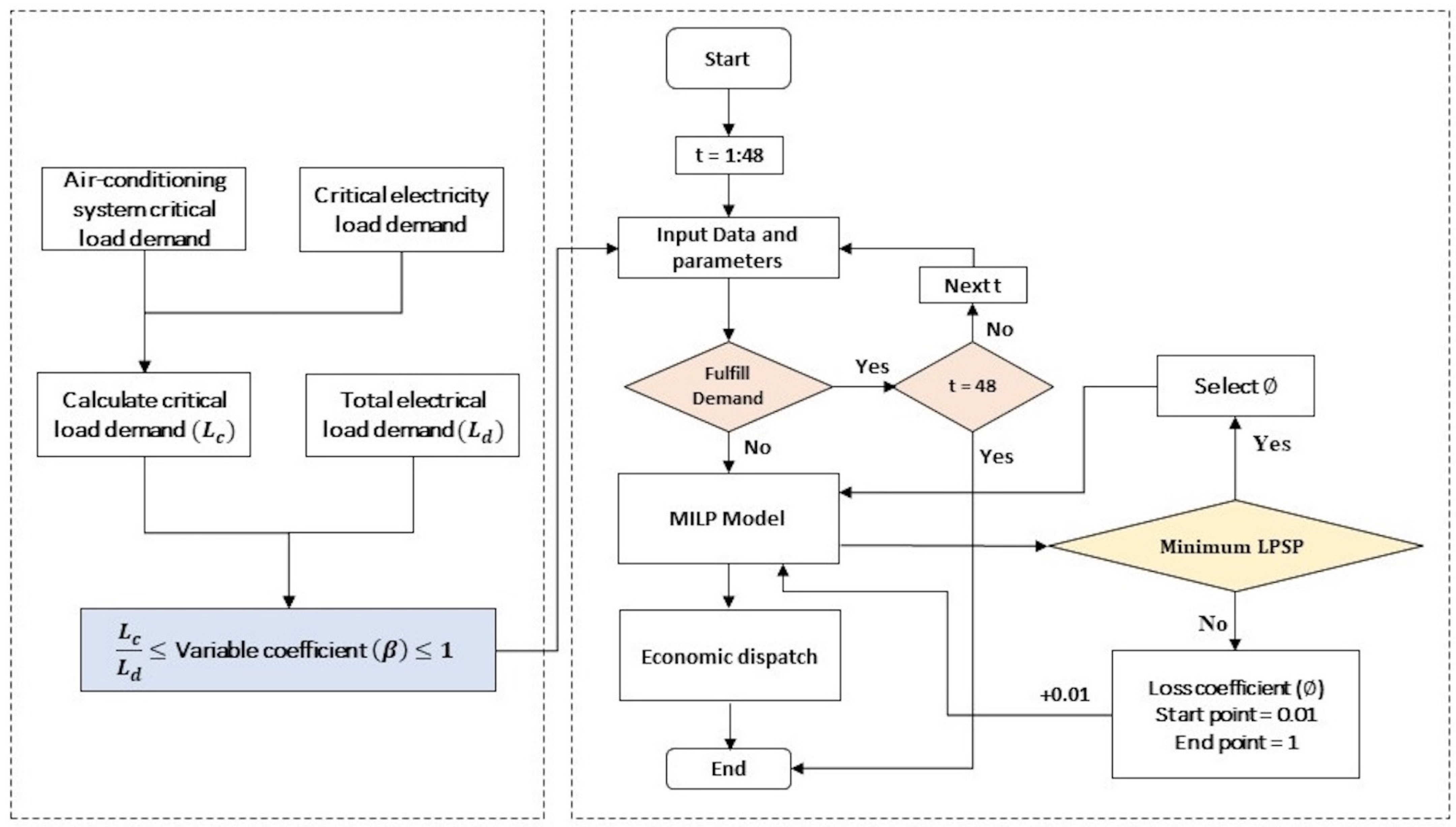
The optimization model used for the economic dispatch (i.e., operation) of the energy system is explained in this section. The main components of the model are a wind turbine, PV panels, and a battery storage system. Figure 1 shows a flowchart for the optimization module. The operation model works with an hourly resolution and a 48 h time horizon.

2.2.1. Objective Function

The economic payoff of the energy system corresponds to its operational cost and its reliability. In this regard, depreciation of the energy storage (batteries), curtailment of renewable energy, and loss of power supply will be key factors in establishing a trade-off between the economy and reliability of the energy system. Although there are other longer-term operation and maintenance (O&M) costs related to the O&M of wind turbines or PV panels, they are not considered in this study, since the focus of this research is on shorter-term operation and maintenance decisions. The elements considered are formulated as follows:

• Battery depreciation:

There are several factors that could affect the depreciation of lithium-ion battery storage systems, such as depth of discharge, charge and discharge cycles, and temperature [20]. The impact of charge/discharge cycles is formulated as a cost indicator (Equation (6)) and added to the objective function.

$$DPC={\displaystyle \sum }_{t=1}^{T}DPF\times Pch\left(t\right)+{\displaystyle \sum }_{t=1}^{T}DPF\times Pdis\left(t\right)$$

(6)

where $Pch\left(t\right)$ and $Pdis\left(t\right)$ are the power of charging and discharging in the time period T, respectively, $DPC$ is the depreciation cost of the battery, and $DPF$ indicates the degradation factor expressed below:

$$DPF=\frac{RC}{C{P}_b}$$

(7)

where the total charge/discharge power capacity of the battery is $C{P}_b$, while $RC$ is the replacement cost of the battery.

• Renewable Curtailment

The main reason for the renewable curtailment could be a mismatch between the time of peak demand and the peak of renewable generation [21]. To improve the economy of the energy system, the amount of excess renewable electricity needs to be minimized by operation management. Therefore, one of the main elements of the objective function is a penalty of the renewable curtailment calculated via Equation (8):

$$RC={\displaystyle \sum }_{t=1}^T\partial \times P_{wc}\left(t\right)+{\displaystyle \sum }_{t=1}^T\partial \times P_{PVc}\left(t\right)$$

(8)

where $\partial$ is the curtailment factor ($/kW) and $P_{wc}\left(t\right)$ is the curtailment of wind power, while $P_{PVc}\left(t\right)$ shows the excess electricity of PV generation in period T.

• Loss of Power Supply

To minimize the loss of power supply probability (LPSP), a term needs to be added to the objective function to penalize the existence of the unmet load in each time step. Therefore, the loss penalty (LP) includes the summation of the amount of unmet load in each time step ($L\left(t\right)$) multiplied by the coefficient ($\varnothing$) as indicated in Equation (9).

$$LP={\displaystyle \sum }_{t=1}^T\varnothing \times L\left(t\right)$$

(9)

Then, the summation of the discussed terms creates the objective function ($OF$):

$$OF=DPC+RC+LP$$

(10)

2.2.2. Constraints

The operating cost of the system is minimized subject to the following constraints:

• Battery capacity: The capacity of the battery storage system in the first time step Eb (1) is equal to the initial state of charge of the battery, while in the following time steps, the capacity of the battery is calculated based on its charge/discharge in that time step (Equation (11)):

$$\{\begin{array}{c}Eb\left(t\right)=SO{C}_{initial} \times C_T t=1\hfill \\ Eb\left(t\right)=Eb\left(t-1\right)+Pch\left(t\right)\ast {\eta }_c-\frac{Pdis\left(t\right)}{{\eta }_d} t=T\hfill \end{array}$$

(11)

where $SO{C}_{initial}$ is the initial state of charge of the battery (%), $C_T$ is the total capacity of the battery (kWh), and ${\eta }_c$ and ${\eta }_d$ are charging/discharging efficiencies, respectively. Furthermore, the state of charge of the battery in each time step ($SOC(t)$) should follow the below inequality:

$$SO{C}_{min}\le SOC\left(t\right)\le SO{C}_{max}$$

(12)

• Renewable generation: To balance the used renewable power in the microgrid and the surplus power, two constraints need to be added for both wind power and PV power generation as follows:

  $$\{\begin{array}{c}{P}_W\left(t\right)=Ewind\left(t\right)+E_{s}Wind\left(t\right)\hfill \\ P_{PV}\left(t\right)=EPV\left(t\right)+E_{s}PV\left(t\right) \hfill \end{array}$$

  (13)

where $Ewind\left(t\right)$ and $EPV\left(t\right)$ are the used wind and PV power in each time step, respectively, while $E_{s}Wind\left(t\right)$ and $E_{s}PV\left(t\right)$ are the surplus electricity of wind and PV generation. $P_W\left(t\right)$ is the total power generated by the wind turbines in time step t and $P_{PV}\left(t\right)$ is the total power generated by the PV panels in time step t.

• Energy balance

The equation that shows the balance between the used renewable generation (supply) in the off-grid mode of the system and the demand (including the load demand and energy that is required to charge the battery) is called the balance constraint, and it is shown by Equation (14):

$$Ewind\left(t\right)+EPV\left(t\right)+Pdis\left(t\right)+L\left(t\right)=L_d\left(t\right)+Pch\left(t\right)$$

(14)

where $L_d\left(t\right)$ is the total load demand in time step t.

2.2.3. Optimal Load

To calculate the load with the upper and lower bounds of the actual load demand and critical load demand, the optimal load in each time step needs to be computed. Since the optimization model is responsible for finding the best value of the load in each time step, a variable has to be defined and added to the balance constraint as shown below (Equation (15)):

$$Ewind\left(t\right)+EPV\left(t\right)+Pdis\left(t\right)+L\left(t\right)=\beta \left(t\right)\times L_d\left(t\right)+Pch\left(t\right)$$

(15)

where $\beta \left(t\right)$ is the variable coefficient. The upper bound ($ub$) of this variable is 1, while the lower bound ($lb$) could be defined based on the proportion of the critical load to the actual load demand.

$$\{\begin{array}{c}lb\left(t\right)=\frac{L_c\left(t\right)}{L_d\left(t\right)}\hfill \\ ub\left(t\right)=1\hfill \end{array}$$

(16)

where $L_c\left(t\right)$ is the critical load in time step t.

2.2.4. LPSP

In this study, loss of power supply probability (LPSP) is employed to evaluate and compare the reliability of the energy system in different scenarios. LPSP could be expressed via Equation (17) below [22]:

$$LPSP=\frac{{{\displaystyle \sum }}_{t=1}^{T}L\left(t\right)}{{{\displaystyle \sum }}_{t=1}^T{L}_d\left(t\right)}$$

(17)

3. Case Study

One of the largest buildings of Concordia University (called EV building), located in downtown Montreal (Quebec), is considered for the case study. Based on the explained methodology, different use types in the EV building with corresponding floor areas are listed in

Table 3. Use categories and their floor areas in EV Building.

Use Type	Floor Area (Ai)	Ratio of Area to Total Area (Ri)	${\mathit{C}}_{\mathit{e}\mathit{d}\mathit{a}\mathit{y}}$	${\mathit{C}}_{\mathit{e}\mathit{n}\mathit{i}\mathit{g}\mathit{h}\mathit{t}}$
Health Center	3427.8	4.1%	1	0.2
computer services	134.6	0.2%	1	1
research labs	7957.9	9.5%	1	1
maintenance services	277	0.3%	1	1
lavatories	1298	1.5%	1	0.5
offices	10,597.3	12.6%	1	1
food services	568.2	0.7%	1	0
offices	5298.6	6.3%	1	0
indoor parking	1647	2.0%	1	0
teaching labs	7328.3	8.7%	1	0
classrooms	1336.8	1.6%	1	0
community services	5413	6.5%	0.2	0
gym	3427.8	4.1%	0.2	0
common areas	24,583.9	29.3%	0.2	0.2
museum	237	0.3%	0.2	0
housekeeping	385	0.5%	0.2	0
others	9896.6	11.8%	0.2	0
Total area (A)	83,814.9	100.0%

[23] to calculate the critical load. The critical coefficients related to electricity demand are shown in $C_{eday}$ and $C_{enight}$ columns.

The EV building has central heating and cooling systems and the critical coefficient regarding air-conditioning (CA) values is assumed as presented in

Table 4. Critical coefficient values for summer and winter.

Coefficient	Value	Time Range
Summer
$C_{day}$	0.4	08:00 to 18:59
$C_{night}$	0.3	19:00 to 07:59
Winter
$C_{day}$	0.6	08:00 to 20:59
$C_{night}$	0.2	21:00 to 07:59

. The coefficients and the time range for day and night are selected based on the working hours of an educational building. It is assumed that in the case of a power outage caused by natural hazards, the air conditioning will be set to a state that meets minimum needs with respect to ventilation and comfort temperature for critical uses such as health centers or research labs inside the building. These coefficients change based on the season, since working hours and space heating and cooling demands are different for summer and winter. These coefficients could also be different from one building to another (even for the same building types) due to the possibility of having different use types with varied characteristics of areas in each building.

4. Input Data

The load demand is randomly selected for two days in winter (15 and 16 February 2019) and two days in summer (14 and 15 July 2019) as representatives of the cold and warm seasons when load demand fluctuates more. The resolution of the load demand is hourly, and the time horizon is 48 h.

The number/capacity of the components in the designed energy system is listed in

Table 5. The microgrid components and battery information.

Component	No./Capacity
Wind Turbine 25 kW (No.)	50
PV Panel 220 W (No.)	13,662
Battery (kWh)	9584
Maximum SOC of the batteries (%)	95
Minimum SOC of the batteries (%)	10
Initial State of Charge (kWh)	8000
Discharging Efficiency (%) [24]	90
Charging Efficiency (%) [24]	95
Maximum charge/discharge rate	0.3
Replacement cost (USD/kWh)	156
Total cycles in the lifetime of each unit [25]	300
Curtailment Factor ($/kW) [26]	0.1

.

Since the microgrid is designed to be grid-connected in the urban area, the renewable penetration is 53%. Therefore, the system requires a sufficient energy management system to control the operation during grid power failure resulting in the loss of power supply.

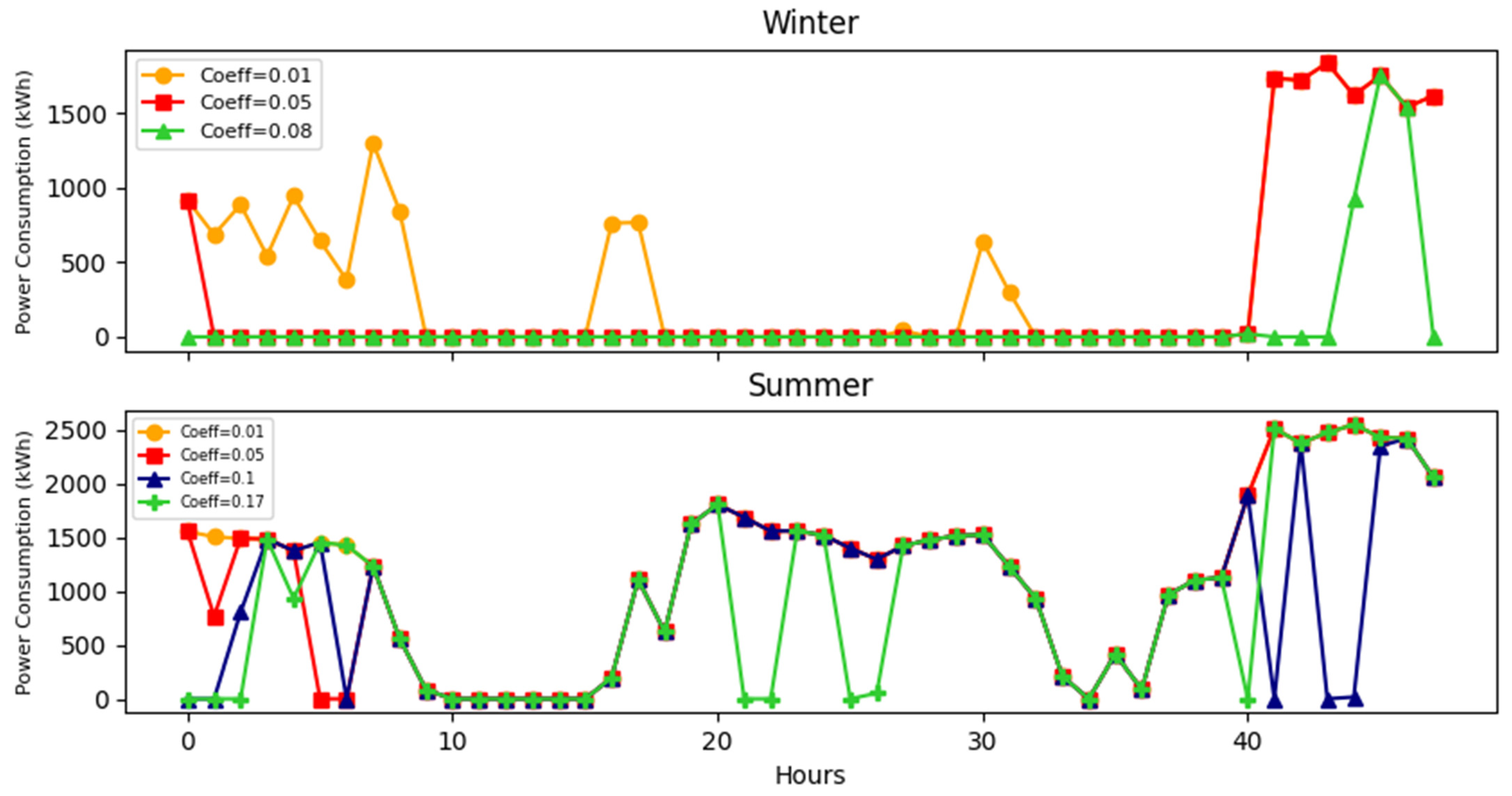
The other important parameter that needs to be set and one that significantly impacts the final results is the loss coefficient ($\varnothing$), with $/kW unit, which is a constant parameter (not changing through the time horizon). Selecting a proper coefficient needs a trial and error process to find an optimal coefficient in the case of both economic and reliability aspects. Therefore, in this research, all possible coefficients in the range of 0.01 to 1 (step = 0.01) are tested. Since the final results of the unmet load only change with certain coefficients (the other coefficients have the same rate and trend of the amount of unmet load (kWh) while having a higher operation cost), the threshold coefficients are selected and are shown in Figure 2. The results show that increasing the penalty for having an unmet load could reduce the loss; however, this increment could cause a considerable rise in the operating cost.

Furthermore, increasing the loss after the maximum thresholds (0.08 and 0.17) will not further affect the loss. Therefore, in this study, the threshold coefficients 0.08 and 0.17 were considered the loss coefficients for winter and summer, respectively. These coefficients have a minimum loss and a minimum cost (compared to the larger coefficients).

5. Results

The optimization model was coded in Python programming language using the Pyomo platform [27]. Since there is no nonlinearity in the model’s equations, and with the presence of binary variables, the mixed-integer linear programming (MILP) method [28] is used to formulate the problem. The CPLEX solver [29] is selected to solve the developed MILP problem.

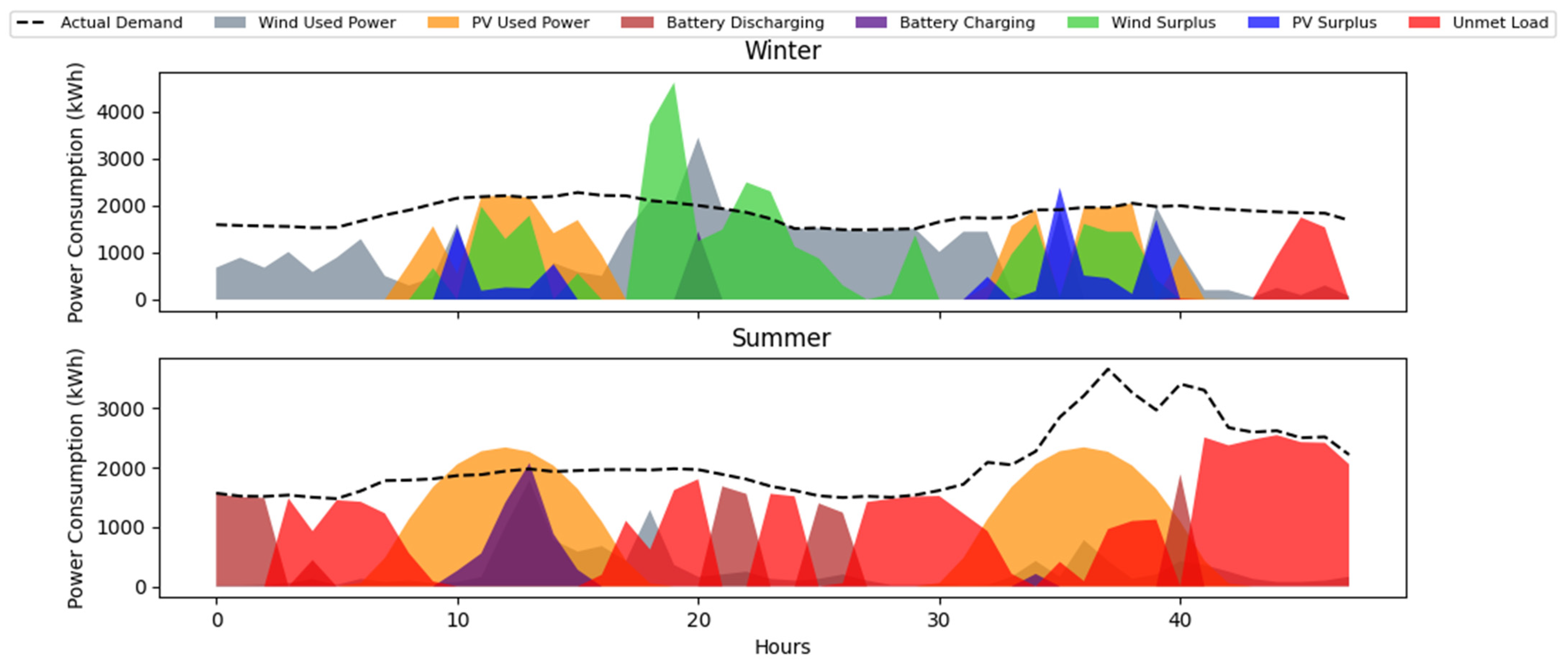
The results of using the actual load demand to find the optimum schedule of the microgrid in the off-grid mode in summer and winter are illustrated in Figure 3. The model’s outcome shows that the amount of wind surplus power in the winter season is considerable in some hours. On the other hand, this amount is negligible on the selected days in summer, since wind power generation is reduced in summer compared to winter. The other noticeable trend is the amount of unmet load in summer, which is significant in most hours. The notable volume of the loss of power supply in summer drastically raises the operational cost (

Table 6. Comparison of the scheduling results for the actual, critical, and optimal loads.

Coverage	Loss Occurrence (No.)	Loss (kWh)	Loss Reduction (%)	LPSP	Operating Cost ($)	Cost Reduction (%)
14 and 15 of July (Summer)	Loss Coefficient = 0.17
Actual Load	34	44452.86	-	0.446	8921.71	-
Critical Load	1	551.94	98	0.012	2565.01	71
Optimal Load	2	551.63	98	0.010	1938.22	78
15 and 16 of February (Winter)	Loss Coefficient = 0.08
Actual Load	4	4226.17	-	0.048	5687.43	-
Critical Load	0	0	100	0	7856.48	−27
Optimal Load	0	0	100	0	4725.89	17

). Furthermore, based on the results in Table 6, the amount of unmet load in winter is also considerable and needs to be diminished.

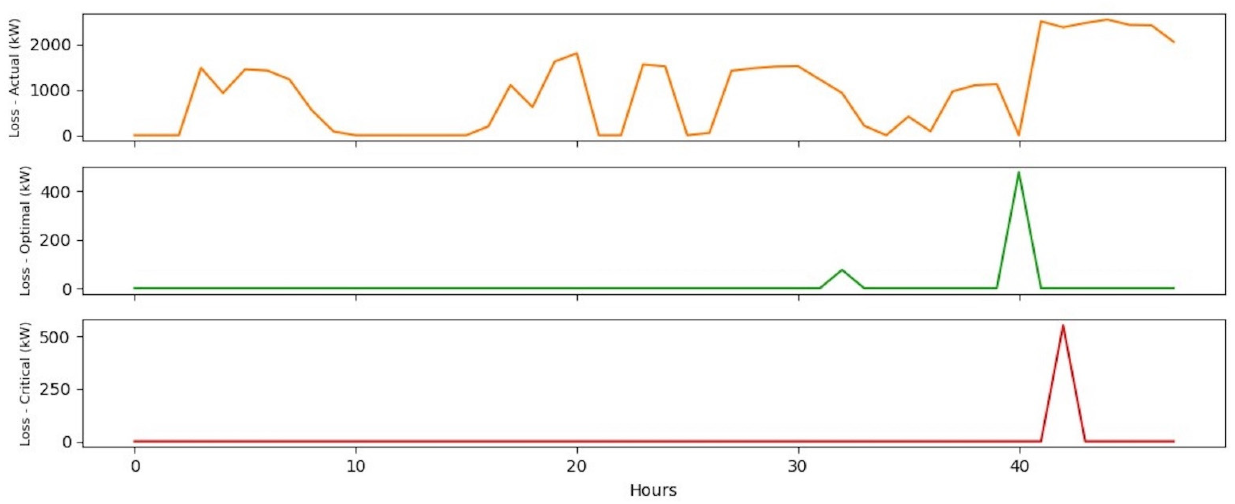
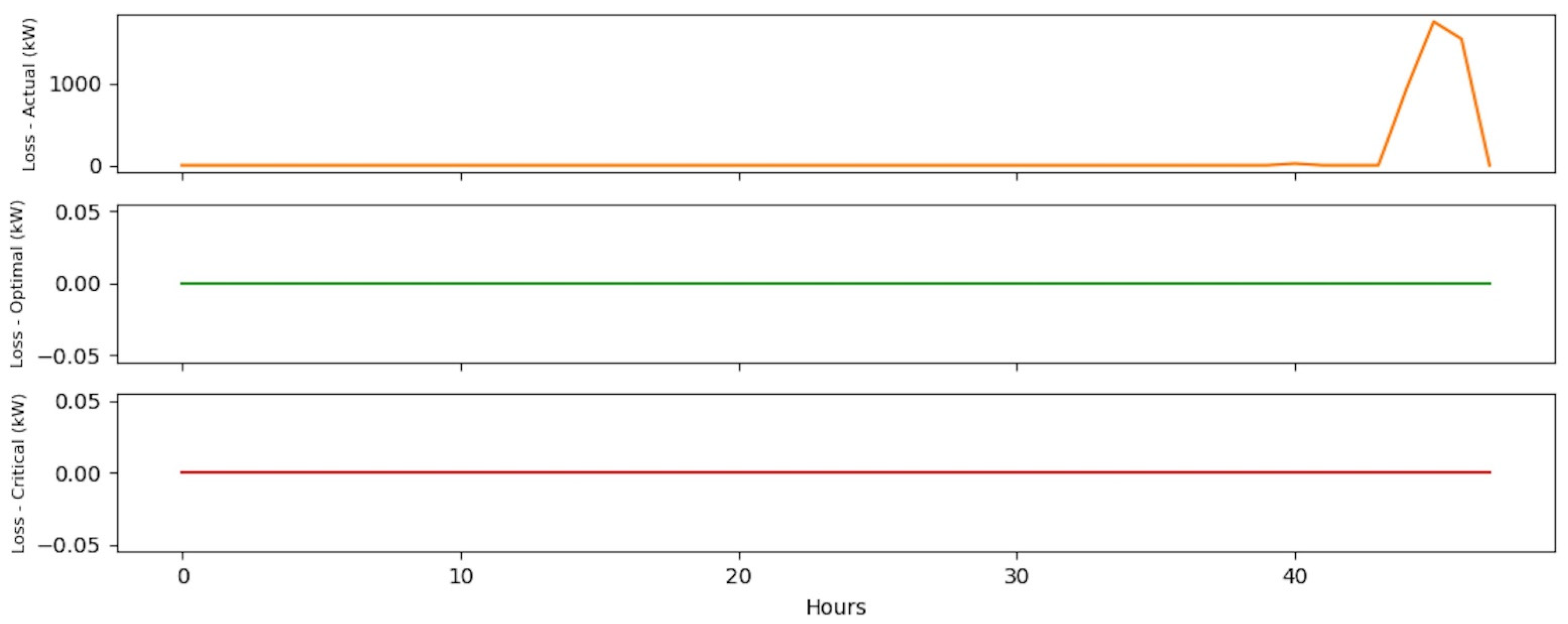
One of the alternatives to lessen the unmet load is using the calculated critical load to at least serve the power to vulnerable sections. Figure 4 and Figure 5 illustrate the number of times that a loss of power could happen and its representing value in an hourly resolution in summer and winter, respectively using actual, critical, and proposed optimal loads. According to these figures, using both critical load and optimal load can reduce the number of power loss occurrences and their values to zero in winter and to a minimum level in summer. Although using a critical load could decrease the loss of power supply probability to a minimum level, in the winter case, it drastically increases the microgrid’s operating cost (Table 6). This growth in operational cost is also mildly observed in summer. The curtailed renewable power growth could explain the increase in operation cost in the winter during different hours.

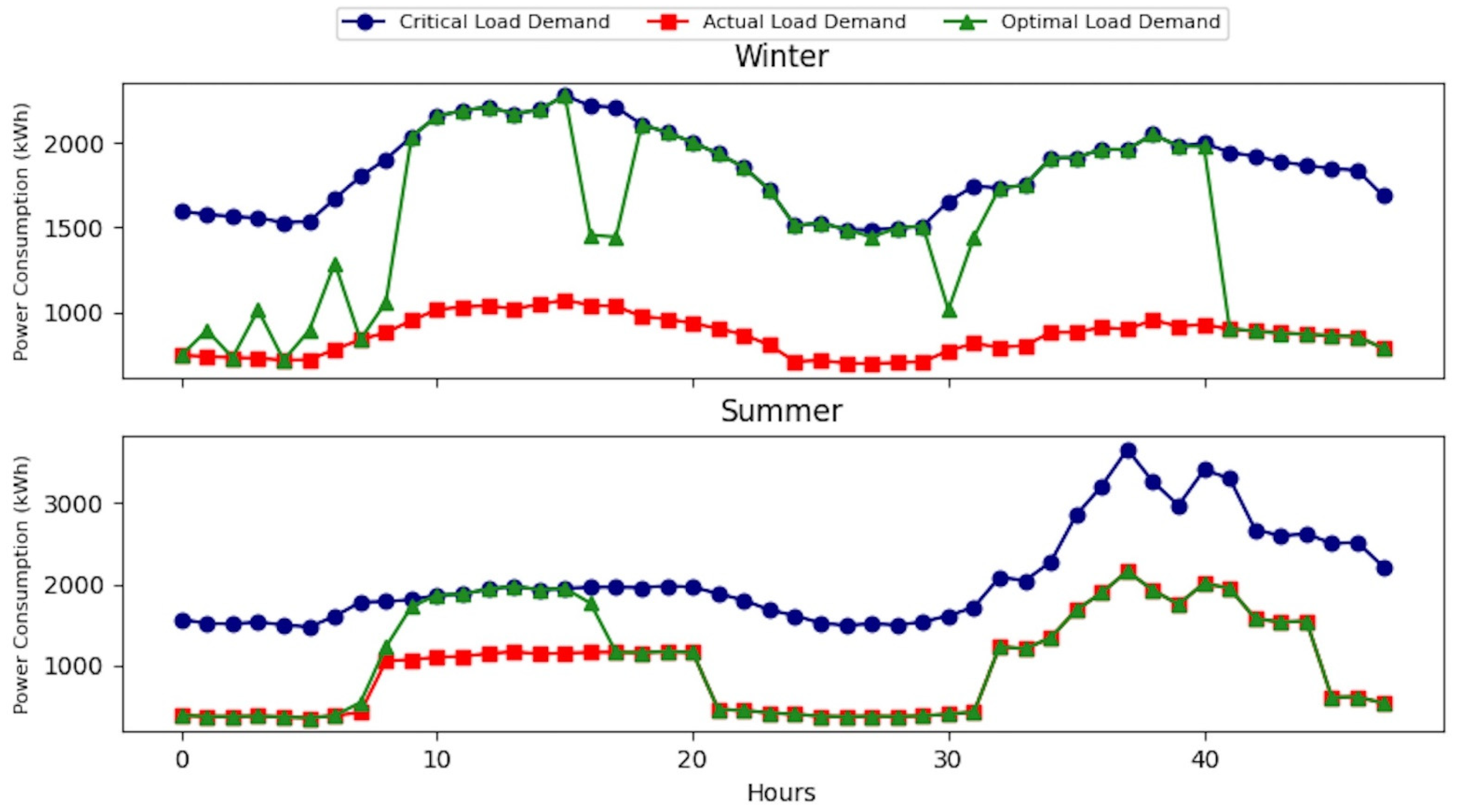
Therefore, to tackle the challenge of having a surplus power penalty caused by using the critical load, the optimal load needs to be calculated by the MILP model to not only bring down the loss of power supply probability but also minimize the operating cost of the system. The optimal loads evaluated by the MILP model for both summer and winter are shown in Figure 6. It is evident from the results that, in winter, the optimal load fluctuates more between the critical load and actual load and tends toward the actual load, while in summer, there is just one fluctuation, and it leans toward the critical load. This could be justified by the amount of renewable generation on different days and the actual load demand. For example, on the second summer day, the actual load demand rises while the amount of renewable generation is insufficient (Figure 3). Therefore, the optimal load tends to be the critical load on this day since this could be the lower limit for the optimal load.

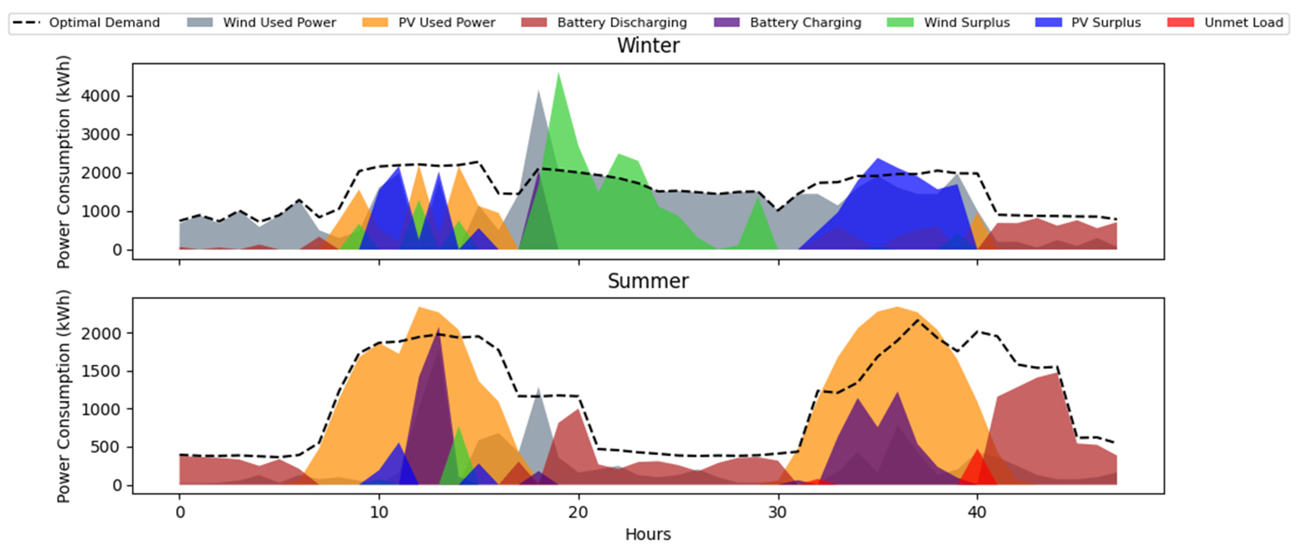
The optimum scheduling results of using the optimal load that the optimization model calculates are shown in Figure 7. Regarding this figure and Table 6, the amount of unmet load in winter is zero and in summer is near zero, while the amount of added surplus power in both seasons is not very considerable compared to the actual load schedule. This will cause a meaningful reduction in the operating cost of the microgrid. Moreover, comparing the optimal load schedule (Figure 7) with the schedule corresponding to the actual load reveals that the amount of battery charge–discharge increases (not significantly) in the case of optimal load in both summer and winter, slightly raising the operational cost.

Based on the results demonstrated in Table 6, employing the optimal load proposed by the optimization model in summer and winter could bring down the operating cost of the microgrid in the off-grid mode by about 78% and 17%, respectively (loss and cost reductions are reported in Table 6 compared to the actual load coverage). Moreover, it could lessen the LPSP to near zero (0.010) in summer and drop it to zero in winter. Although using optimal load has reduced the operating cost of the microgrid in winter to 4725.89$ from 5687.43$, this change is not significant compared to that in summer (reducing operating cost from 8921.71$ to 1938.22$). This is due to variations in renewable generation over those randomly selected days in summer and winter. Since the amount of wind power generation for the chosen day in summer is much less than that of the selected day in winter, the amount of unmet load in summer is considerably higher (44,452.86 kWh) compared to winter (4226.17 kWh).

6. Conclusions

In this study, the aim was to propose an approach for reducing the risk of power failure in urban microgrids by improving resilience while minimizing operation cost. In particular, employing a two-step process is proposed to reduce the cost while improving reliability. Step 1 considers a penalty for loss and calculating the optimum penalty factor, and Step 2 finds an optimal load demand that can be covered by the microgrid during the off-grid mode. The results indicate that with the proposed method, the LPSP of the system could be significantly reduced to near zero, and the amount of loss could drastically diminish (17% and 78% in winter and summer, respectively). Furthermore, using optimal load, the amount of curtailed renewable power was controlled and remained at the minimum level. The proposed method also minimized the system’s operating cost compared to other scenarios.

Potential future research could integrate forecasting load demand and renewable generation models to remove the uncertainty of using historical data. Moreover, the effect of considering a more resilient design on operation management could also be explored. Critical load calculation subject to the day and night coefficient assumptions could be done based on the real data to increase the accuracy of the operation model.

References

- Li, Z.; Shahidehpour, M.; Aminifar, F.; Alabdulwahab, A.; Al-Turki, Y. Networked Microgrids for Enhancing the Power System Resilience. Proc. IEEE 2017, 105, 1289–1310. [Google Scholar] [CrossRef]
- Panteli, M.; Pickering, C.; Wilkinson, S.; Dawson, R.; Mancarella, P. Power System Resilience to Extreme Weather: Fragility Modeling, Probabilistic Impact Assessment, and Adaptation Measures. IEEE Trans. Power Syst. 2017, 32, 3747–3757. [Google Scholar] [CrossRef] [Green Version]
- Hossain, A.; Pota, H.R.; Hossain, J.; Blaabjerg, F. Evolution of microgrids with converter-interfaced generations: Challenges and opportunities. Int. J. Electr. Power Energy Syst. 2019, 109, 160–186. [Google Scholar] [CrossRef]
- Mishra, S.; Anderson, K.; Miller, B.; Boyer, K.; Warren, A. Microgrid resilience: A holistic approach for assessing threats, identifying vulnerabilities, and designing corresponding mitigation strategies. Appl. Energy 2020, 264, 114726. [Google Scholar] [CrossRef] [Green Version]
- Borghei, M.; Ghassemi, M. Optimal planning of microgrids for resilient distribution networks. Int. J. Electr. Power Energy Syst. 2021, 128, 106682. [Google Scholar] [CrossRef]
- Rigo-Mariani, R.; Sareni, B.; Roboam, X.; Turpin, C. Optimal power dispatching strategies in smart-microgrids with storage. Renew. Sustain. Energy Rev. 2014, 40, 649–658. [Google Scholar] [CrossRef] [Green Version]
- Kong, X.; Xiao, J.; Liu, D.; Wu, J.; Wang, C.; Shen, Y. Robust stochastic optimal dispatching method of multi-energy virtual power plant considering multiple uncertainties. Appl. Energy 2020, 279, 115707. [Google Scholar] [CrossRef]
- Shirzadi, N.; Nasiri, F.; El-Bayeh, C.; Eicker, U. Optimal dispatching of renewable energy-based urban microgrids using a deep learning approach for electrical load and wind power forecasting. Int. J. Energy Res. 2021, 46, 3173–3188. [Google Scholar] [CrossRef]
- Augustine, N.; Suresh, S.; Moghe, P.; Sheikh, K. Economic dispatch for a microgrid considering renewable energy cost functions. In Proceedings of the 2012 IEEE PES Innovative Smart Grid Technologies (ISGT), Washington, DC, USA, 16–20 January 2012; pp. 1–7. [Google Scholar]
- Lu, X.; Liu, Z.; Ma, L.; Wang, L.; Zhou, K.; Feng, N. A robust optimization approach for optimal load dispatch of community energy hub. Appl. Energy 2020, 259, 114195. [Google Scholar] [CrossRef]
- Daneshi, H.; Khorashadi-Zadeh, H. Microgrid energy management system: A study of reliability and economic issues. In Proceedings of the 2012 IEEE Power and Energy Society General Meeting, San Diego, CA, USA, 22–26 July 2012. [Google Scholar] [CrossRef]
- Costa, P.M.; Matos, M.A. Economic Analysis of Microgrids Including Reliability Aspects. In Proceedings of the 9th International Conference on Probabilistic Methods Applied to Power Systems KTH, Stockholm, Sweden, 11–15 June 2006. [Google Scholar]
- Hussain, A.; Bui, V.-H.; Kim, H.-M. Resilience-Oriented Optimal Operation of Networked Hybrid Microgrids. IEEE Trans. Smart Grid 2019, 10, 204–215. [Google Scholar] [CrossRef]
- Zakernezhad, H.; Nazar, M.S.; Shafie-Khah, M.; Catalão, J.P. Optimal resilient operation of multi-carrier energy systems in electricity markets considering distributed energy resource aggregators. Appl. Energy 2021, 299, 117271. [Google Scholar] [CrossRef]
- Garcia-Torres, F.; Valverde, L.; Bordons, C. Optimal Load Sharing of Hydrogen-Based Microgrids With Hybrid Storage Using Model-Predictive Control. IEEE Trans. Ind. Electron. 2016, 63, 4919–4928. [Google Scholar] [CrossRef]
- Tobajas, J.; Garcia-Torres, F.; Roncero-Sánchez, P.; Vázquez, J.; Bellatreche, L.; Nieto, E. Resilience-oriented schedule of microgrids with hybrid energy storage system using model predictive control. Appl. Energy 2022, 306, 118092. [Google Scholar] [CrossRef]
- DHS; R. S. Committee. DHS [Department of Homeland Security] Risk Lexicon; DHS: Washington, DC, USA, 2010. [Google Scholar]
- Chalishazar, V.; Poudel, S.; Hanif, S.; Mana, P.T. Power System Resilience Metrics Augmentation for Critical Load Prioritization; Pacific Northwest National Lab. (PNNL): Richland, WA, USA, 2021. [Google Scholar] [CrossRef]
- For, A.; Release, P.; Unlimited, D. Unified Facilities Criteria (Ufc) Approved for Public Release; Distribution Unlimited Engine-Driven Generator Systems for Prime\1\and Standby Power Applications/1. 2014. Available online: http://dod.wbdg.org/ (accessed on 3 October 2022).
- Zia, M.F.; Elbouchikhi, E.; Benbouzid, M. Optimal operational planning of scalable DC microgrid with demand response, islanding, and battery degradation cost considerations. Appl. Energy 2019, 237, 695–707. [Google Scholar] [CrossRef]
- Yan, X.; Zhang, X.; Gu, C.; Li, F. Power to gas: Addressing renewable curtailment by converting to hydrogen. Front. Energy 2018, 12, 560–568. [Google Scholar] [CrossRef]
- Hosseini, S.J.A.D.; Moazzami, M.; Shahinzadeh, H. Optimal sizing of an isolated hybrid wind/PV/battery system with considering loss of power supply probability. Majlesi J. Electr. Eng. 2017, 11, 63–69. [Google Scholar]
- Archidata. Available online: https://fmis.concordia.ca/ (accessed on 3 October 2022).
- Wen, L.; Zhou, K.; Yang, S.; Lu, X. Optimal load dispatch of community microgrid with deep learning based solar power and load forecasting. Energy 2019, 171, 1053–1065. [Google Scholar] [CrossRef]
- Tektronix. Lithium-Ion Battery Maintenance Guidelines. 2000. Available online: http://www.newark.com/pdfs/techarticles/tektronix/LIBMG.pdf (accessed on 17 October 2022).
- Xu, X.; Hu, W.; Cao, D.; Huang, Q.; Liu, W.; Liu, Z.; Chen, Z.; Lund, H. Designing a standalone wind-diesel-CAES hybrid energy system by using a scenario-based bi-level programming method. Energy Convers. Manag. 2020, 211, 112759. [Google Scholar] [CrossRef]
- Hart, W.E.; Watson, J.-P.; Woodruff, D.L. Pyomo: Modeling and solving mathematical programs in Python. Math. Program. Comput. 2011, 3, 219–260. [Google Scholar] [CrossRef]
- Wolsey, L.A. Mixed Integer Programming. In Wiley Encyclopedia of Computer Science and Engineering; Wiley: Hoboken, NJ, USA, 2008; pp. 1–10. [Google Scholar] [CrossRef]
- IBM ILOG. CPLEX User’s Manual; IBM ILOG: Gentilly, France, 2017; p. 596. [Google Scholar]
Figure 1.
A schematic design of the optimization module.
Figure 2.
Trial and error results for finding the best coefficient.
Figure 3.
Optimal Schedule using actual load demand.
Figure 4.
Loss occurrence and value in Summer.
Figure 5.
Loss occurrence and value in winter.
Figure 6.
Optimal, actual, and critical loads for summer and winter.
Figure 7.
Optimal Schedule using optimal load demand.