
Data-Driven Virtual Replication of Thermostatically Controlled Domestic Heating Systems
by
 , , , ,
Gerard Mor
1 ,
,
Jordi Cipriano
1,2,
Eloi Gabaldon
1,
Benedetto Grillone
3,
Mariano Tur
4 and
Daniel Chemisana
2,* 1
Building Energy and Environment Group, Centre Internacional de Mètodes Numèrics a l’Enginyeria, CIMNE-Lleida, Pere de Cabrera 16, Office 2G, 25001 Lleida, Spain
2
Applied Physics Section of the Environmental Science Department, University of Lleida, Jaume II 69, 25001 Lleida, Spain
3
Building Energy and Environment Group, Centre Internacional de Mètodes Numèrics a l’Enginyeria, GAIA Building (TR14), Rambla Sant Nebridi 22, 08222 Terrassa, Spain
4
BAXI.BDR-Thermea, Salvador Espriu, 9, 08908 L’Hospitalet de Llobregat, Spain
*
Author to whom correspondence should be addressed.
Energies 2021, 14(17), 5430; https://doi.org/10.3390/en14175430
Submission received: 23 July 2021
/
Revised: 10 August 2021
/
Accepted: 24 August 2021
/
Published: 1 September 2021
Abstract
:Thermostatic load control systems are widespread in many countries. Since they provide heat for domestic hot water and space heating on a massive scale in the residential sector, the assessment of their energy performance and the effect of different control strategies requires simplified modeling techniques demanding a small number of inputs and low computational resources. Data-driven techniques are envisaged as one of the best options to meet these constraints. This paper presents a novel methodology consisting of the combination of an optimization algorithm, two auto-regressive models and a control loop algorithm able to virtually replicate the control of thermostatically driven systems. This combined strategy includes all the thermostatically controlled modes governed by the set point temperature and enables automatic assessment of the energy consumption impact of multiple scenarios. The required inputs are limited to available historical readings from smart thermostats and external climate data sources. The methodology has been trained and validated with data sets coming from a selection of 11 smart thermostats, connected to gas boilers, placed in several households located in north-eastern Spain. Important conclusions of the research are that these techniques can estimate the temperature decay of households when the space heating is off as well as the energy consumption needed to reach the comfort conditions. The results of the research also show that estimated median energy savings of 18.1% and 36.5% can be achieved if the usual set point temperature schedule is lowered by 1 °C and 2 °C, respectively.
1. Introduction
In 2019, the final energy consumption of the residential sector accounted for 26% of the overall final energy consumption in the EU [1]. The main use of this final energy was for space heating, representing around 64% [1]. Most EU Member States rely mainly on natural gas and electricity for meeting these needs, followed by renewable energies, mostly solid bio fuels. This high dependence on natural gas clearly determines any achievable strategy to reach the binding carbon targets. As stated in [2], energy saving is one of the easiest ways to save money for consumers and to reduce greenhouse gas emissions. The EU has set binding targets of at least 32.5% improvement in energy efficiency by 2030. To achieve this increase in energy efficiency on the global scale, more effort in energy conservation strategies or in electrification of buildings’ technical systems should be dedicated to this endeavor. The electrification can be based on several mature technologies, such as electricity driven heat pumps, hybrid heat pumps, or district heating networks. Many research studies have focused on demonstrating their cost effectiveness and how these technologies can increase the energy efficiency in several European countries [3,4,5,6,7]. This strategy is the best option in the mid-long term. However, in the short term, cost-efficient strategies, able to drastically reduce the energy consumption of legacy space heating systems and, in particular, thermostatically driven systems (fed with gas), should be also accelerated.
Another challenge to address is related to the users’ involvement in the energy transition. Although the technologies are readily available, the control strategy, as well as the involvement of end users in their management is not fully clarified yet. End users must be part of the solution, and this can only be achieved if manufacturers of home space heating/cooling systems, which should be one of the drivers of the low-carbon transition, can find new and more interactive ways to support end customers. The unfolding of these user driven energy control strategies requires higher digitization of the existing systems. Manufacturers should accelerate the virtualization (digital twins) of the operation of their systems to drastically improve the user interaction and the automatic demand response. This process needs some kind of Advanced Metering Infrastructure (AMI) or a massive adoption of smart home devices. To date, Member States committed to rolling out close to 200 million smart meters for electricity and 45 million for gas by the end of 2020 at a total potential investment of EUR 45 billion [8]. By the end of 2021, it is expected that almost 72% of European consumers should have a smart meter for electricity, while 40% should have one for gas.
On the other hand, for the few last years we have seen a fast penetration of the emerging Internet of Things (IoT) technologies into residential homes. Nowadays, smart devices are inevitable in our lives [9,10]. Smart thermostats are one of them. These smart thermostats allow remote control of the home climate, display of the temperature and energy consumption in real time or communication with intelligent cloud-based IT systems to incorporate self-learning capabilities. These are crucial features to accommodate efficient techniques to increase the energy efficiency of space conditioning systems and decrease energy costs. However, some studies [11] showed that 40% of programmable thermostats are used in manual modes, mainly due to confusing user interfaces. Peffer et al. [12] stated significant failures in people–technology interactions when they set their programmable thermostats. They also pointed out some of the needed characteristics to overcome the misconceptions about thermostat operation. For instance, to provide accessible web portals or mobile applications or to add voice recognition features, or indicators of how much time the heating system needs to achieve a desired temperature. Although smart thermostats include some of these features, which help increase the user’s satisfaction, some studies [13] reflect that the end users are still reluctant to rely on the smart thermostat to control their boiler or heat pump. In [14], product reviews of five smart thermostats were collected and analyzed. When comparing the most commonly discussed topics, generally they were not related to energy and cost saving. The most discussed topics were control, ease of use, and installation. In [13] a comparison of two different smart thermostats included an evaluation of the achieved gas savings. The main conclusion was that there appeared to be higher gas savings in homes where the occupancy detection features were enabled. Data gathered by connected thermostats are also useful in understanding the operational and occupancy patterns of users. A longitudinal analysis [15] was conducted in relation to thermostat operation behavior due to the climate, season, and price and to the thermal preferences. It was used to categorize users based on operation. Furthermore, a study [16] on residential households located in high-rise buildings, using complementary survey data, demonstrated the potential benefit of using connected thermostat data as a diagnostic tool to identify opportunities for energy savings in this type of building. In [17], various models designed to predict the user occupancy, based on machine learning and deep learning methods, are compared. Optimal set point temperature scenarios can be also estimated using these occupancy prediction models.
Therefore, while thermostats’ capabilities to control the indoor temperature, mainly based on occupancy detection, are well understood, less is known about their effectiveness to enable energy savings. The uncertainty in relation to the potential energy savings is increasingly important because manufacturers are adding many new features and functions to the thermostats without detailed assessment of their impact on the gas or electricity consumption. Previous research studies demonstrated a high variation in the achieved energy savings due to the substitution of conventional thermostats with smart thermostats. In [18], an assessment of two smart thermostat models is performed, and a high variation of the achieved energy savings, among users with the same smart thermostat, is documented. Moreover, although these smart thermostats were focused on occupancy-responsive control, the specific actions which led to the energy savings as well as the reasons of these high variations are not clearly determined. In [19,20], more detailed assessments of the energy savings achieved by occupancy responsive thermostat control are performed. A clear relationship between this occupancy-based control and the achieved energy savings, supported by supervised learning data-driven models, can be found. Nonetheless, the effect of other control variables such as variations in the set point temperature are not analyzed in detail. Some studies, performed by the National Research Council Canada in their experimental set up (CCHT twin houses), analyzed the effect of thermostat setback strategies over the energy consumption [21]. They tested three setback strategies for the winter season and two more for the summer season. Their research conclusion was that these strategies can be very effective in winter but not in the summer. The research was very accurate in evaluating setback strategies; however, they were tested in non-occupied and highly controlled home environments and they were limited to the applied setback schedules. They did not include dynamic modeling calibration or advanced thermostatically controlled strategies. More research in prediction and control optimization techniques, addressing the uncertainty in the evaluation of the effect over the energy consumption, are certainly necessary.
The prediction and control optimization models should be able to include not only the occupancy and the weather-dependent variables but also the control variable which, in most cases, is the set point temperature. In [22], a review of the state of the art of dynamic models able to predict natural gas consumption, from 2000 to 2010, was presented. From this review, it can be ascertained that an exponential increase in papers was detected in this field, especially in the lower forecasting area level (regional, gas distribution and individual). The predominant trend of these research works was a combination of optimization tools with more classic forecasting models. After 2010, several authors continued using statistical and stochastic methodologies to predict and characterize aggregated gas consumption of residential units or groups of commercial buildings [23,24]. At the individual level, in [25] Nonlinear Mixed-Effects models (NLME) are used for the prediction of single gas consumption at daily basis. After comparing the results among auto regressive models, such as AutoRegressive with eXogenous variables (ARX) and AutoRegressive Moving Average with eXogenous variables (ARMAX) models, the conclusion was that such models perform similarly but have both merits and problems. The NLME models are cleaner and clearer, while ARX and ARMAX are better for local adaptation to sudden and abrupt changes within a single individual. In [26], linear ARX, Artificial Neural Networks (ANN) and Support Vector Machine Models (SVM) are applied to forecast natural gas consumption on a daily basis. The solar radiation as an exogenous variable was included in the models and the accuracy improved. That research work performed a very detailed evaluation of several Time Series (TS) models in non-occupied test homes and clearly quantified the model accuracy improvement by introducing the solar radiation as an exogenous variable. The results were encouraging, however these test conditions were very far from real and occupied buildings where the heating system is thermostatically controlled by the user through the set point temperature. In [27], a step wise calibration of a dynamic thermal empirical model of a residential building was performed. The calibration included some user-dependent parameters, such as the air ventilation rates; however, the constraints derived by the set point temperature control were not included in the analysis. More recently, Wang et al. [28] developed a home thermal dynamic model built upon the standard Resistance and Capacitance (R-C) approach and tested it with data from a test home in free-floating conditions. This R-C model included the effect of most of the exogenous variables, such as the internal and external temperatures, the wind direction and the solar radiation, though it did not consider the effect of the set point temperature and of the user behavior. Alinberti et al. [29] developed a non-linear Autoregressive Neural Network model for short and medium-term predictions of the indoor temperature of a secondary school building. The accuracy of the predictions is very well evaluated; however, as in the previous literature works, the model cannot evaluate the effect of the set point temperature in the energy consumption. In [30] a machine learning model to predict residential energy consumption based on data from Wireless thermostats is developed. Although the results are very promising in relation to the energy savings evaluation, the developed technique requires many data of the building features and it is limited to monthly frequency. This could be a clear limit for wider application and for near-real time control solutions.
Recent studies moved one step beyond the prediction of the energy performance of thermostatic load control systems and assessed control-optimized techniques within Demand Response (DR) programs or in relation to the electricity network operation [31]. In [32], the set point temperature of thermostatically controlled systems is included in the evaluation of the demand response programs in 1000 households. That paper is based on synthetic data; however, it demonstrated how an accurate modeling of the thermostatic control of space heating and cooling systems enables simple and reliable evaluation of demand response and of Energy Conservative Measures (ECM) in the residential sector. These emerging applications require very fast and computation efficient data-driven models able to provide the necessary response.
From these previous research works, it can be concluded that, although the knowledge of the energy performance of thermostatic load controlled systems is growing fast, there are still some gaps in relation to the modeling of the combined effect of the thermal energy supplied by the heating system, of the user-based thermostatic control driven by the set point temperature and of the exogenous variables (external weather conditions). Furthermore it is also stated that more advanced modeling strategies, able to virtually mimic the performance of the thermostatic control, are needed if we want to increase the smartness of these systems and to enhance interactions with the customers. In our research, a new methodology to emulate the performance of thermostatic load controlled systems is developed and put in practice. The novelty relies on the fact that, unlike most literature solutions, which limit their applicability to forecasting the indoor temperature or the energy consumption separately, our approach combines several optimization techniques, with auto regressive models and a control loop, to model cross-combined effects and to mimic all the possible control modes driven by the control variable (the set point temperature). The control loop included in the methodology is based on the difference between the indoor and the set point temperatures. The mode when the indoor temperature is higher than the set point threshold is modeled by a first regression model where the indoor temperature is the dependent variable and the space heating power consumption is one of the input variables. This space heating power consumption becomes a dependent variable, fed by the indoor temperature and other exogenous variables, when the indoor temperature is lower than the set point temperature threshold. Both regression models are combined to forecast the expected energy consumption and the potential energy savings when a certain set point temperature schedule is applied. The methodology was validated in real cases within a heating season. However, a similar implementation should be applicable also to space cooling system as long as they are thermostatically-controlled systems.
The paper starts with a mathematical description of the regression models and of the input variables transformation. It follows with a description of the processes used to train both models and to optimize the regression parameters. The procedure used to combine the two regression models to predict the energy consumption, and the potential energy savings due to a certain set point temperature schedule, is then described. The paper finishes with the application of the methodology over a set of households in northeastern Spain, which are equipped with condensing gas boilers driven by smart thermostats.
2. Methodology
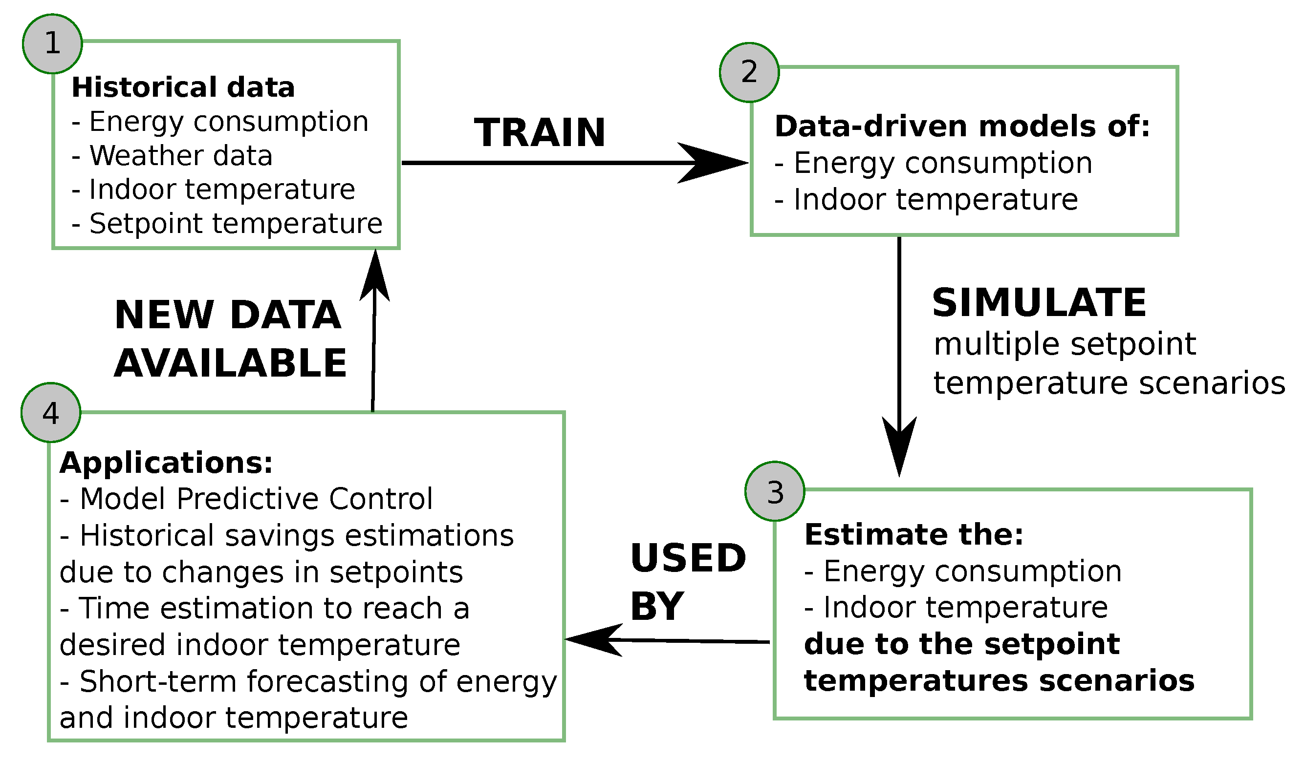
The energy performance of a household is influenced by many factors that include the dynamic indoor and outdoor conditions, the physical and geometric characteristics of the building, the type of space conditioning system and, finally, the control of this system, which in most cases is a thermostat controlled by the end-users. Therefore, when modeling the energy performance of real households using data-driven models, all these factors should be considered. In this paper, a methodology is developed to accurately predict the energy consumption and indoor temperature of thermostatically controlled heating systems. Technically, the methodology combines two ARX models, named the demand-side and the supply-side models, in order to dynamically simulate the heat losses and gains of the building due to changes in the thermostat set point temperature. The demand-side model captures the heat dynamics affecting the indoor temperature of the household, while the supply-side model determines the heat dynamics concerning boiler energy consumption. The two models, and their control loop coupling, are trained using historical data of real systems performance during occupancy. Figure 1 depicts the general flow diagram of the developed methodology. The first step starts with the gathering of historical data available from smart thermostats reading and from weather forecasting web services which provide climatic data. Then, both data-driven models are trained using these data sets. Subsequently, these models are used as a simulation tool to estimate the energy consumption and indoor temperature due to changes in set point temperatures. Finally, the set of validated algorithms can be used for multiple smart-control applications, such as Model Predictive Control (MPC) or short-term forecasting. The outputs of these applications, in turn, can generate more data which can be fed into an iterative self-learning process to re-train the models.
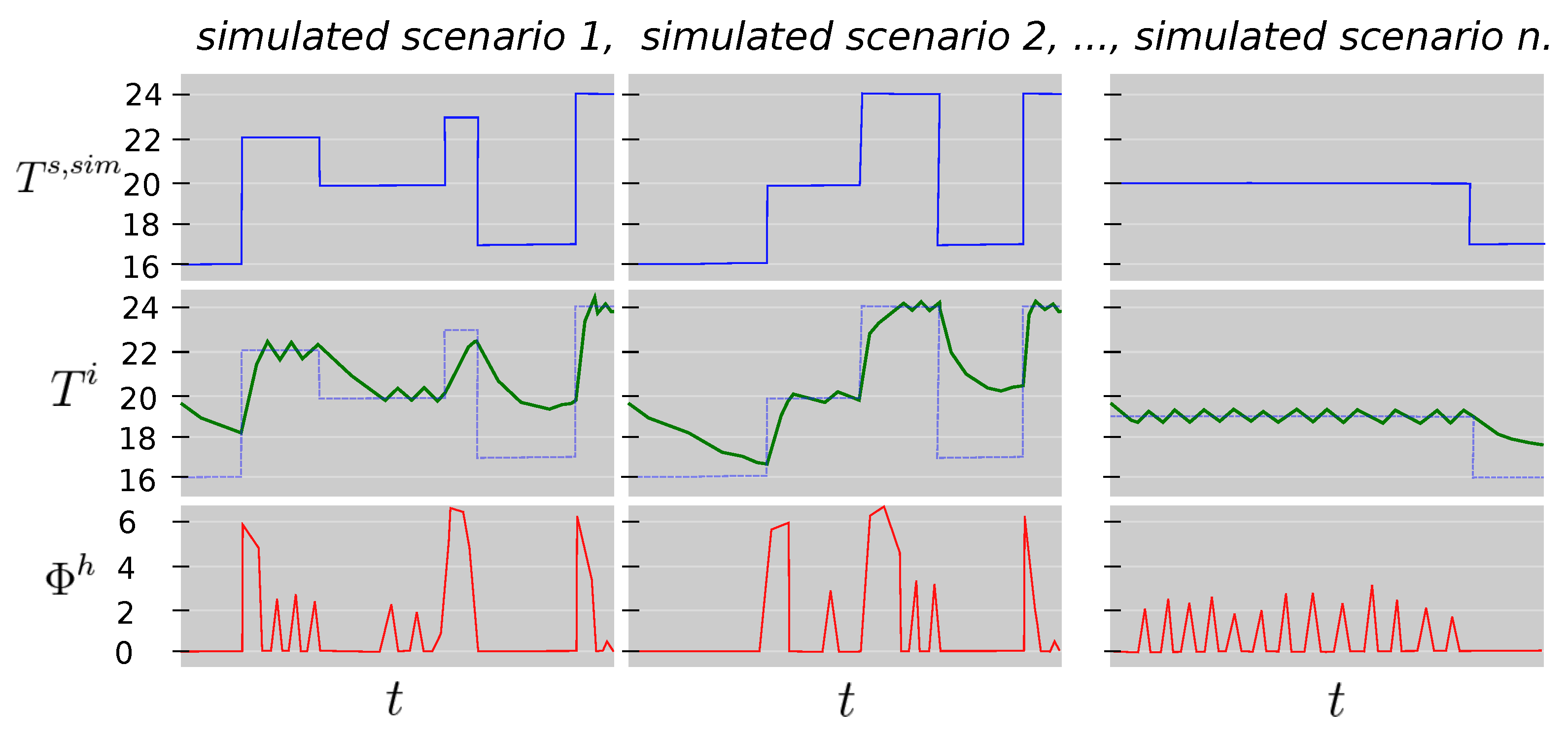
The use of two models is justified because the heat dynamics of the building are not affected by only the external variables and the supplied energy. They are also affected by the indoor conditions. The lower the indoor temperature, the higher the energy to be supplied to reach the comfort conditions defined by the set point temperature thresholds. One of the models, the demand-side model, is used to simulate the indoor temperature of the household in free-floating conditions, when energy delivered by the heating system is zero. The other model, the supply-side model, is used to estimate the energy needed to recover the indoor comfort conditions when the supply system is activated again. Figure 2 shows 3 different scenarios of simulated set point temperature schedules, , the corresponding simulated indoor temperature changes, and the supply energy delivered by the gas boiler to recover the comfort conditions, . As can be seen, the length of the free-floating periods determine the indoor temperature decay and the energy to be supplied by the gas boiler consumption to reach the set point temperature schedule again. ARX models were selected, because these kind of black-box models contain autoregressive impulse responses which can properly describe time-varying processes in a fast and efficient way. In addition, as can be seen in Section 2.5, a hybrid optimization procedure, considering least squares and a Genetic Algorithm (GA), is applied to fit the models and to identify the unknown parameters. Last but not least, in Section 2.3, a description of the prior transformations applied to several input variables, along the training phase, are presented.
2.1. Demand-Side Model
The demand-side model is defined by an ARX model represented by the indoor temperature () as the output. The external weather conditions and the space heating consumption are the input variables. This model captures how the heat flows out of the building and how the indoor temperature is affected by the space heating system. The model formula is described in Equation (1).
The autoregressive terms , , , and the coefficients and are the parameters of the model. Regarding the first group, they are defined in Equation (2), where: n is the number of lags, or order, of the backward shift operator B, defined as . y is the considered variable, for instance, the indoor temperature in the case of or the outdoor temperature in .
The independent variables considered in the model are:
- Time-lagged (n) indoor temperatures () to characterize the inertia of the building.
- Low-pass filtered outdoor temperature () to characterize the heat loses through the envelope of the building due to changes in the outdoor temperature.
- Raw outdoor temperature () to consider fast changes in indoor temperatures due to changes in the daily minimum and maximum temperatures.
- Heat consumption of the boiler () to characterize the increase in the indoor temperature due to the operation of the heating system.
- Solar direct normal irradiance (), interacting with the Fourier series of the solar azimuth () and of the solar elevation () to characterize the solar gains of the building.
- Wind speed (), interacting with Fourier series of the wind direction () and the temperature difference between indoors and outdoors () to characterize the heat losses due to air leakage and convection effects through the envelope.
2.2. Supply-Side Model
This dynamic model estimates the amount of energy needed to warm up the household considering the inertia of the building, the external weather conditions, the performance of the boiler and its thermostatic control.
In this model, , , are the autoregressive terms and , are the linear parameters of the model. The output is the log-transformed consumption . The inputs of the model are:
- Time-lagged (n) heat consumption () to consider how the boiler was performing in the last time steps.
- Raw data of the outdoor temperature () to consider the variation of the coefficient of performance of the boiler due to changes in the outdoor temperature.
- is the low-pass filtered version of the outdoor temperature. It represents the temperature of the building envelope.
- As in the demand-side model, the solar direct normal irradiance () interacts with the Fourier series of the solar azimuth () and of the solar elevation ().
- as in the case of the demand side model, it is the temperature difference between indoors and outdoors.
- Wind speed () interacts with Fourier series of the wind direction () and the temperature difference between indoors and outdoors ().
Unlike the demand-side model, the data sets used to estimate the and parameters only consider the periods where . This is because no information can be extracted about the performance of the boiler in the periods that it is not operating.
2.3. Transformation of Input Variables
2.3.1. Low-Pass Filter
The application of a Low-Pass Filter (LPF) over the exogenous variables, used as inputs of the models, transforms them into variables that better represent the dynamics of the system and, therefore, the model fitting is improved. The LPF assumes that the dynamics of the buildings can be described by lumped parameter R-C models; see for example [33,34]. This assumption means the response of the indoor temperature or the energy consumption to changes in some climate exogenous variables can be modeled as a first order LPF. Based on this assumption, it is reasonable to apply LPF to all the exogenous variables in order to eliminate the high input frequencies that might negatively affect the model training. The discrete time implementation of this first order R-C LPF is the exponentially weighted moving average of each variable with the filter parameter () tuned to match the response of the building to each effect separately:
where is the filtered exogenous variable, is the filter parameter , and x is the original time series of the exogenous variable.
2.3.2. Fourier Series
The correlation between indoor temperature (), solar irradiance () and air leakage () is, normally, non-linear. Multiple reasons lead to this behavior, such as: building envelope orientation and characteristics, sun position and wind direction. To solve this issue, a harmonic function, based on a Fourier series, is used to account for these non-linearities. Solar azimuth , solar elevation and wind direction are the observations transformed using this technique, and the number of harmonics considered are, respectively, , and .
In Equation (6), Y represents the observation to be transformed, is the transformed variable, is the maximum number of harmonics included in the Fourier series , and are the regressors of each component. In the demand and the supply-side models, the generic coefficients depicted in Equation (6) are identified following the same procedure as , , and parameters
2.4. Models Coupling
The supply-side and the demand-side models are coupled to allow the simulation of both the space heating energy consumption and the indoor temperature, given a certain set point temperature schedule.
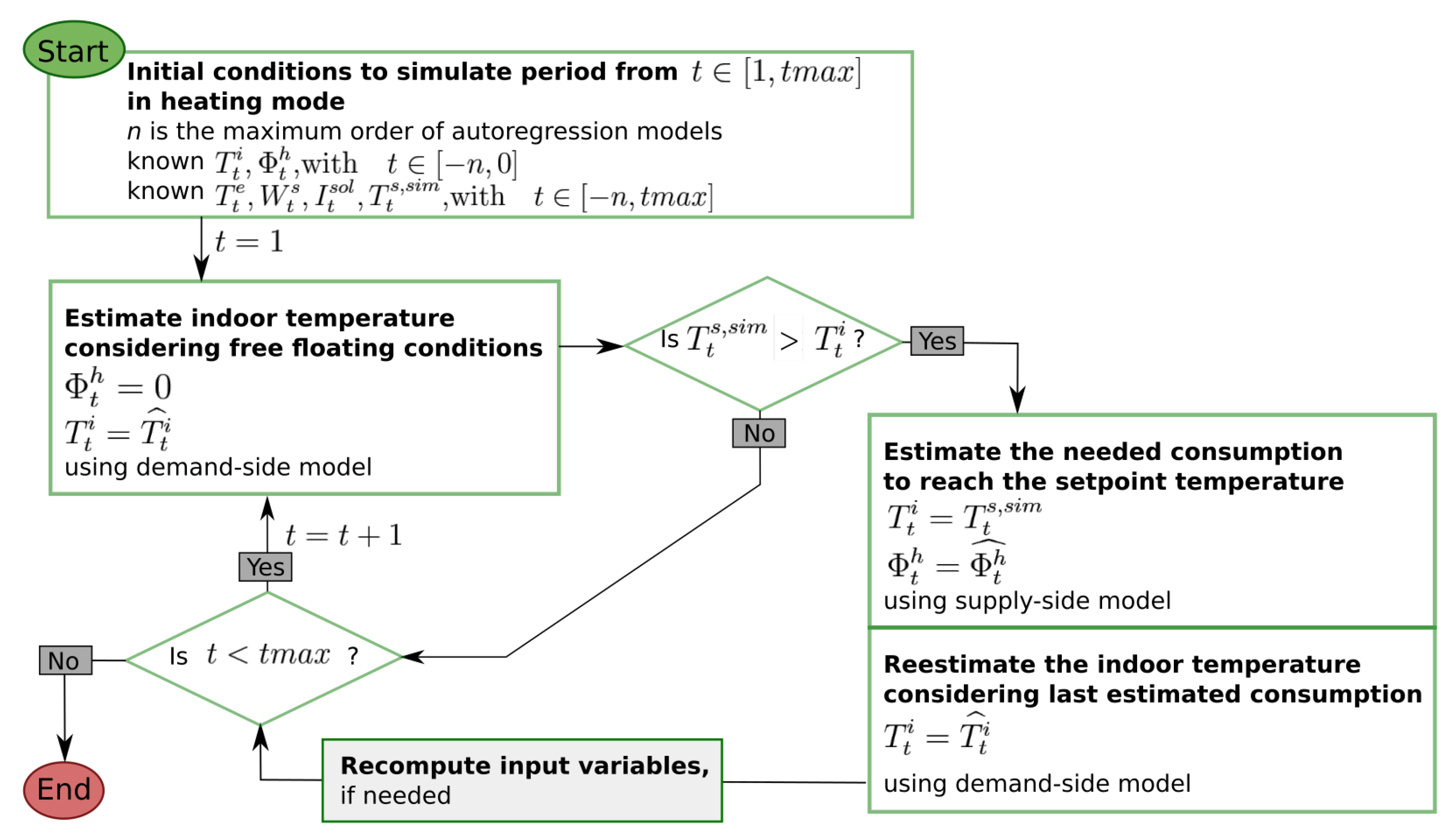
Figure 3 accurately describes how the models are coupled (Algorithm A1 of the Appendix A). In essence, it mimics the operation of a thermostat considering the heat transfers of a household and setting on or off the operation of the boiler according to the set point temperature. At each time step, the algorithm predicts the variation of the indoor temperature in free-floating conditions, and then, when the set point temperature is higher than the indoor temperature, it simulates the space heating operation by estimating both the energy consumption and the indoor temperature the household will reach.
2.5. Model Training and Parameter Optimization
The linear least squares method is used to estimate the , , and parameters of both ARX models. However, there are more parameters to be optimized: the coefficients of the input feature transformations and the auto regressive orders of the ARX models. Those parameters cannot be estimated using the least squares method used in the regression analysis. Therefore, a Genetic Algorithm (GA) technique is used as the optimizer for those coefficients. The GA evaluates several combinations of a set of coefficients and then estimates the remaining ones (, , and ) using the least squares method. The cost function is defined in Equation (7). The GA is based on the R package GA, developed by Scrucca et al. [35,36]. The GA package provides a flexible general-purpose set of tools for implementing a genetic algorithm search in both the continuous and discrete case, whether constrained or not. In this research, a binary GA is selected within the available tools of the GA package. A binary GA is a simple and flexible optimizer able to simultaneously include multiple integer, continuous and discrete variables. More specifically, a Reflected Binary Code (RBC) representation, which is an ordering of the binary numeral system such that two successive values differ in only one bit, is used as the binary representation of each chromosome evaluated by the GA. This RBC enhances the optimization process during the recombination and mutation steps. Algorithm A2 describes in detail this optimization procedure. Algorithm A3 describes the way in which the cost of each chromosome is calculated during the evaluation steps of Algorithm A2. The cost function considered in this optimization is defined in Equation (7). It consists of a combination of the Coefficient of Variation of the Root Mean Squared Error (CVRMSE) of the indoor temperature and of the space heating energy consumption. Although the CVRMSE is not affected by zero values of the boiler energy consumption, it is only computed for households with aggregated historical energy consumption greater than zero, . As can be seen in Algorithm A3, the cost of each chromosome is evaluated using the cross-validation folds along a testing period.
Once all the parameters are optimized, the supply-side and the demand-side models are considered as correctly validated and are ready to be used for further evaluations.
2.6. Evaluation of Potential Energy Savings
The developed methodology is suitable for multiple applications. For instance, day-ahead forecasting or Demand Response (DR) services can benefit from this methodology by including it within Model Predictive Control (MPC) procedures. To demonstrate its wider applicability, within the framework of this paper, the assessment of several set point temperature scenarios along a historical period, is performed.
These scenarios are always compared against the Business as Usual (BaU) scenario, instead of against the real data measurements. The reason is that the models errors, even if they are small, may disturb the evaluation of the estimated absolute energy differences. Therefore, it is better to compare between simulated scenarios and to obtain relative energy differences that are affected by the same error model. This strategy is supported by the fact that both the demand side and the supply model residuals fulfil the white noise requirement. The model parameters were trained using a cross-validated framework and, finally, the models were validated over a data set not seen by any of the cross-validation folds. The only requirement to assure an accurate evaluation of the relative energy differences is that the set point temperature, along the training period, should contain different temperature levels. This guarantees proper capturing of the heat dynamics of the households. Therefore, if no excitation is provided to the output variables, no dynamics can be inferred. Equation (8) describes the mathematical expression used to evaluate the relative energy differences between a BaU scenario, in which the set point temperature is the same as the measured one, (), and another scenario under evaluation, represented by .
3. Case Study
Case Study Datasets
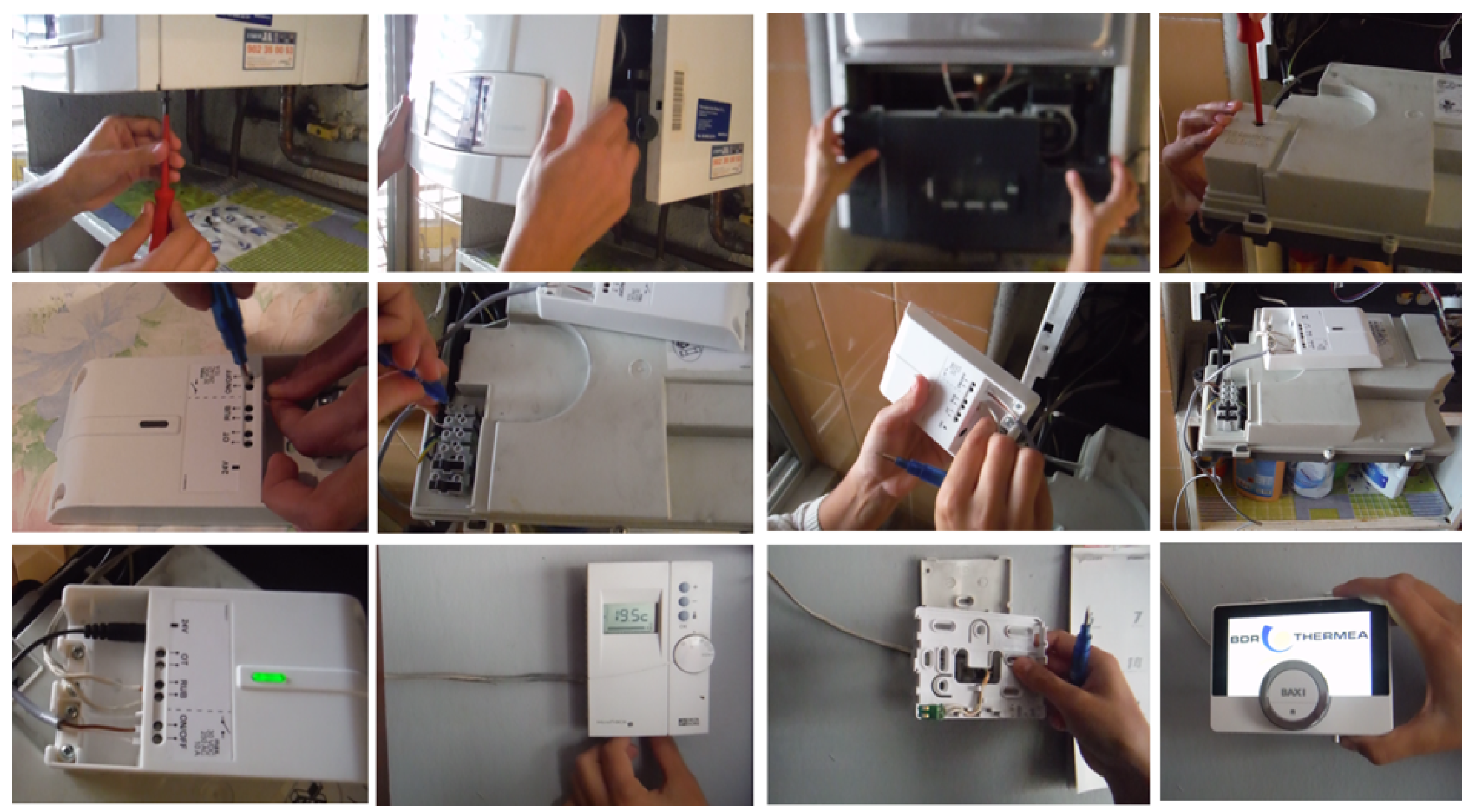
A real test of the whole methodology was performed over a test pilot case formed by 15 households placed in a north-western area of Spain. Each household is equipped with a condensing gas boiler which is controlled by a smart thermostat. Both the condensing boiler and the smart thermostat, named BAXI Connect, were manufactured and provided by the company BAXI. In all cases, the distribution heating systems were based on radiators. Other building characteristics as well as occupancy patterns were not known because of data privacy requirements. Figure 4 shows a set of pictures of the installation process. It starts with the connection between the control board and the gateway, followed by the removal of the old thermostat and finishing with the switching on of the new smart thermostat. The smart thermostat follows the Open Therm communication protocol to communicate with the gas boiler and a wireless connection to communicate with the household router. The variables transmitted by the thermostat are: the indoor temperature, the set point temperature, the outdoor temperature (boilers equipped with an extra sensor), an indirect estimation of the space heating thermal power, and an indirect estimation of the domestic hot water thermal power. These data are communicated every 60 min and the hourly measurement tolerance corresponds to 1 kWh for the space heating and domestic hot water power and 0.5 °C for the temperature readings. The testing period started in December 2018 and finished in May 2019. However, since the involved customers had to accept the terms and conditions through the BAXI Connect mobile application, the activation was performed sequentially in time. A representative number of connected customers was not achieved until March 2019. Therefore, the analyses performed in this research are limited to this time period, from March to May. The final number of users with accurate data had to be limited to 11 households, selected among the whole population of 15 households. This reduction is due to the lack of data availability for the selected test period and due to the requirement of having a minimum level of excitation of the set point temperature. Several heating and cooling ramps were required for proper model training. Households where the set point temperature was fixed along large periods (several days, weeks, or even months) were discarded.
The IT architecture of this case study is formed by the local smart thermostat which transfers all the data to a central server managed by BAXI. These data were anonymized and communicated through a RESTful API communication layer to the big data analytics cloud. The details of this distributed and big data processing framework are described in [37].
Climate Data
Although some of the households have an extra temperature sensor placed outside the building to provide data on climate-dependent exogenous variables, the amount of gaps and outliers discarded the use of these data. As an alternative, outdoor temperature, wind speed and wind bearing data were obtained from a weather web service managed by the company Dark Sky [38]. These climate data are based on the approximate location of each household (postal code). Additionally, the global incident solar radiation on a planar surface is obtained from the Copernicus European Union’s Earth observation program [39], which entails more accurate modeling the solar heat gains of the households.
4. Results
4.1. Detailed Model Validation in One Household
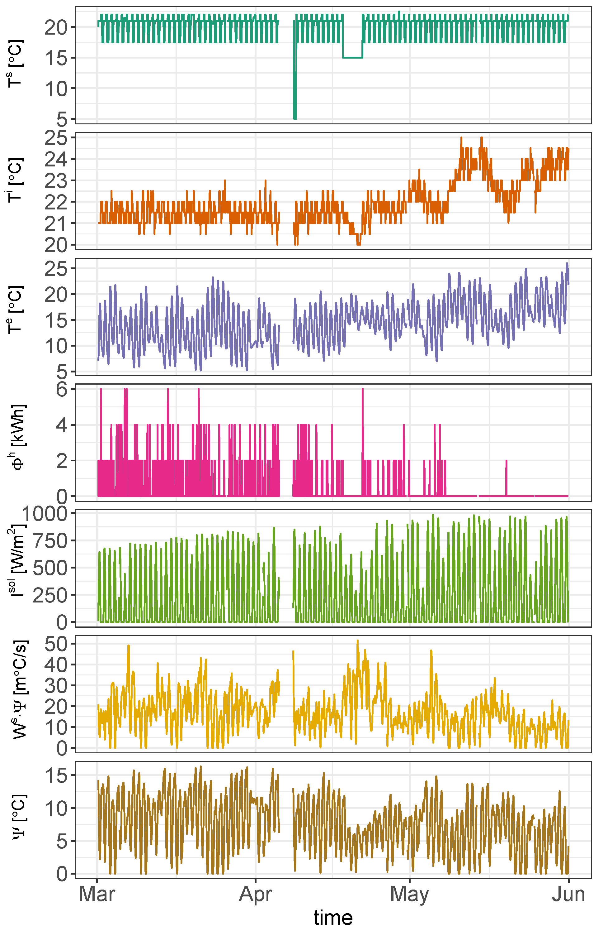
In Figure 5, the variables used in the demand and supply-side models of one of the analyzed households are shown. The testing period ranges from 1st March to 31st May 2019. Starting from the top, the dark-green line corresponds to the set point temperature assigned by the tenant. The dark-orange line corresponds to the indoor temperature gathered by the thermostat. The violet line corresponds to the outdoor temperature gathered from dark sky web service [38]. The outdoor temperatures, ranging between 10 °C and 25 °C, are observed along the testing period. The magenta line corresponds to the boiler energy consumption. The light-green line corresponds to the direct normal incident solar radiation. The dark-yellow line represents the wind speed times. The light-brown line corresponds to the difference between the outdoor and the indoor temperatures, only if this is positive. In addition, Figure 6 depicts the set point and the indoor temperature for the same household, but in a shorter period. The aim is to show the correct operation of the thermostatic control.
Using these initial data sets, a cross-validation process is implemented to identify all the unknown parameters of the two models. The number of folds () considered was eight, and the percentage of training in each fold was 80%. The ranges, and the allowed levels considered for the optimization are summarized in Table 1. As can be seen, most of the obtained auto-regressive orders have a maximum value of four because beyond this value their statistical significance tends to decrease. However, in the case of the indoor temperature, since this state variable is highly affected by the household thermal inertia, higher orders are permitted in the optimization (7 and 16 in the supply-side and demand-side, respectively). The ranges of harmonics for the Fourier series are between one and three. These ranges keep the model simple while allowing enough flexibility. To increase the chances of the GA obtaining larger values of the alphas and to address their high sensibility when they have values close to one, an exponential weighted distribution was permitted. The set of optimal parameters for the household in study is described in the last right-hand column of Table 1.
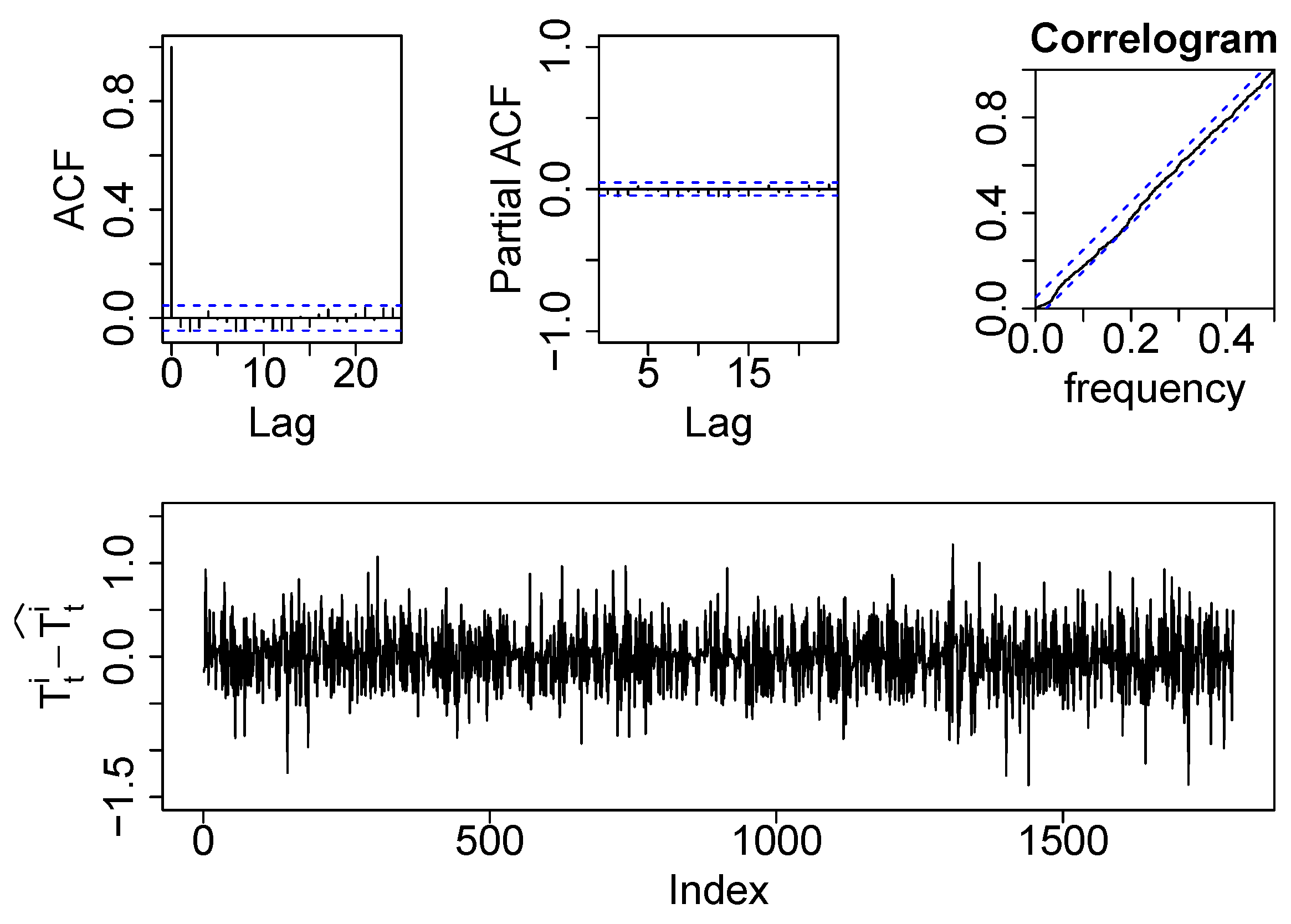
Figure 7 shows the residual analysis of the demand-side model of the analyzed household along the training period. As can be observed, the residuals are not auto-correlated, they follow a Gaussian distribution and the variance is homocedastic along the time. These three conditions set that the residuals are independent and identically distributed, meaning they achieve the white noise condition and the model is properly trained and considered as valid. To validate the model with new data, and therefore to assess its forecasting accuracy, the daily aggregated and indicators were computed. They yield values are 1.4% and 0.45 °C, respectively. These error ranges are very satisfactory and demonstrate the validity of the model for simulations of long term periods.
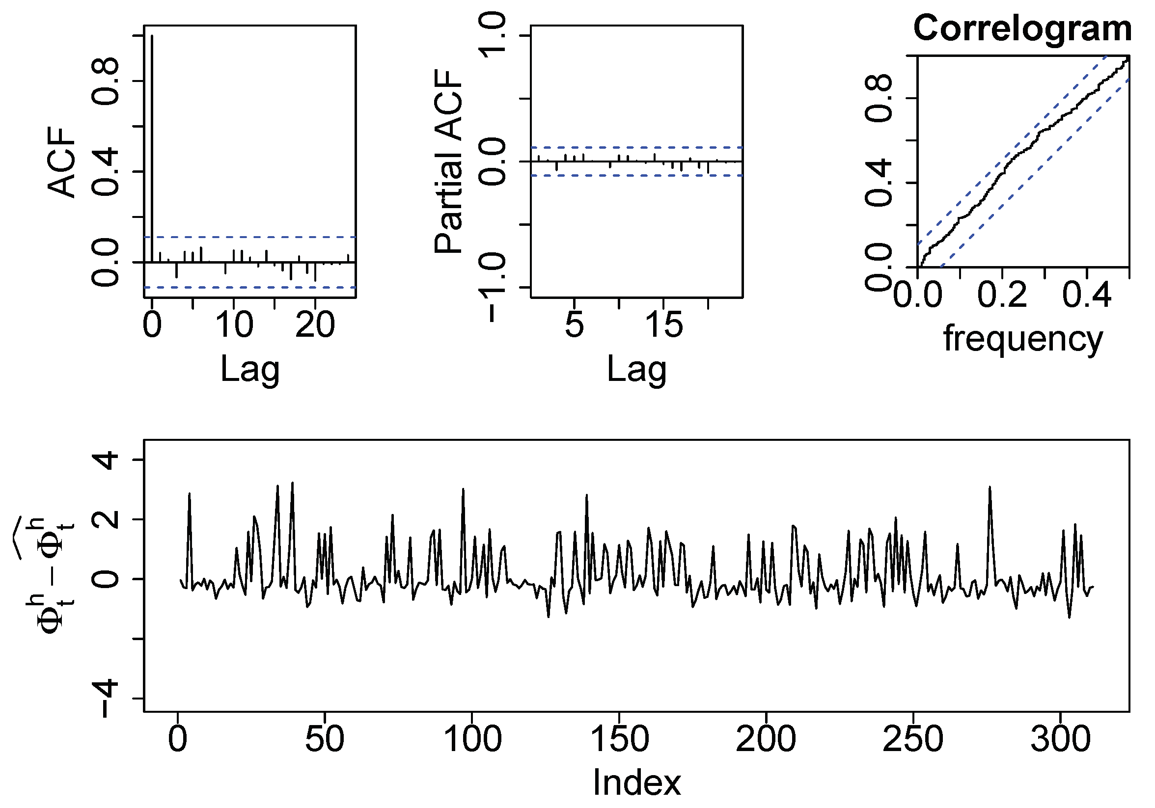
Figure 9 shows the residual analysis of the supply-side model of the analyzed household for the training data sets. As can be observed, the residuals are not auto-correlated, they follow a Gaussian distribution and the variance is homocedastic along the time. These three conditions set that the residual are independent and identically distributed (i.i.d.), meaning they achieve the white noise condition and the model is properly trained and considered as valid. To evaluate the accuracy of the model to assess potential energy savings, the and were computed at aggregated daily granularity. This is because the tolerance of the space heating consumption readings is too high in relation to the hourly space heating consumption of the households. The computed daily and were 37.1% and 4.72 kWh, respectively, for the testing period. These high error values are caused by the high tolerance of the space heating energy consumption readings (1 kWh) and suggest that, for this specific household, long term predictions of potential energy savings are too uncertain.
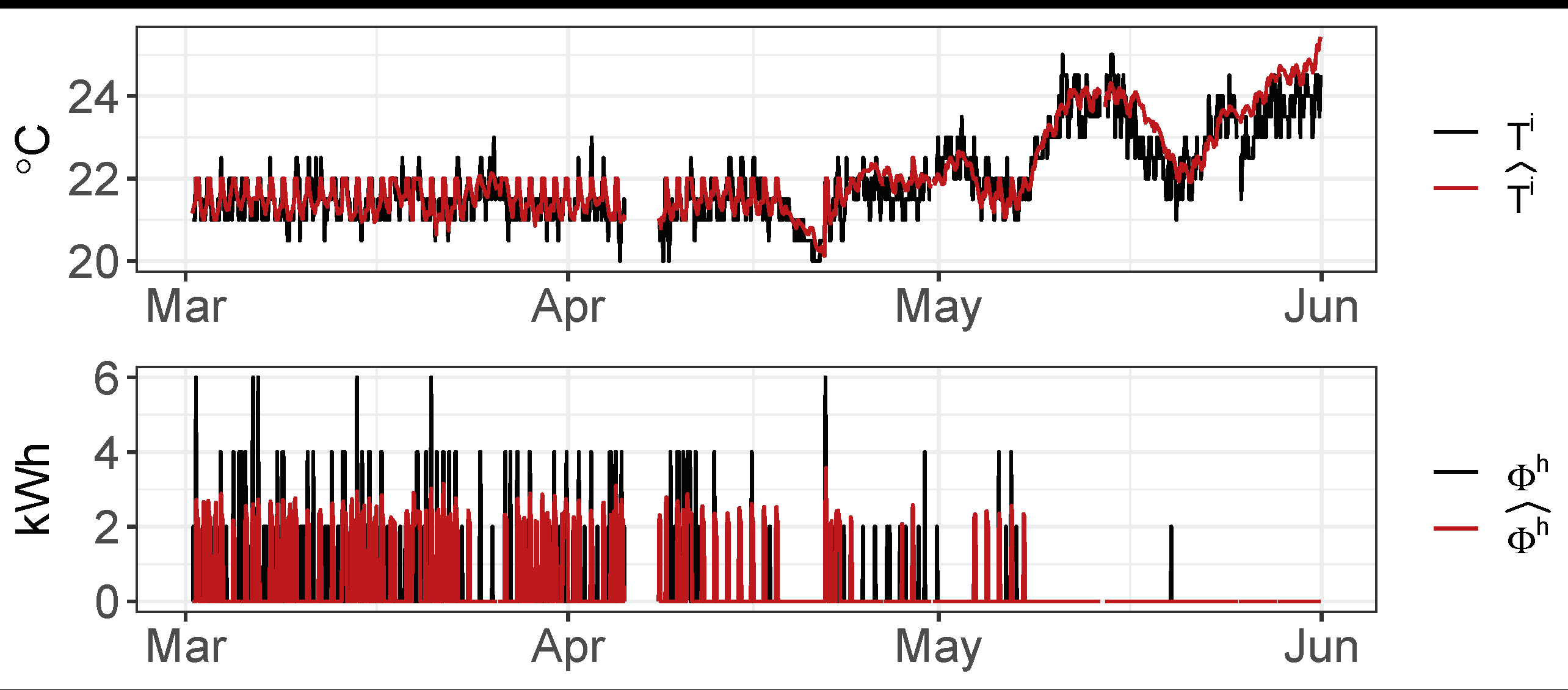
Once the models of the household are trained and validated, forecasts of the indoor temperature and of the space heating consumption are performed, applying the procedure defined in the Algorithm A1. The prediction period was between 1st March and 31st May. Figure 10 depicts the comparison between measured data of heat consumption and indoor temperature , with the black colored line, and the forecasted ones, and , with the red colored line. The set point temperature considered in the forecasting () is the BaU set point (), which is the original schedule set by the user. As can be seen in Figure 5, the set point temperature ranges from 18 °C to 22 °C along the majority of the period. Looking at the results of the simulation, it is notably appreciated that the predicted indoor temperature accurately fits the dynamics of the measured values. However, the supply-model tends to inaccurately predict some of the peaks. As previously mentioned, one of the reasons for this low accuracy is related to the high measurement tolerance of the space heating energy consumption readings. Nonetheless, it is remarkable that the whole-= period aggregated space heating energy consumption difference () is 12 kWh. That means only 1.55% over-prediction, which can be considered as a good result considering the main goal of this research.The good performance of the models in periods where the household behaves in free-floating mode (with the boiler switched off) is also remarkable.
4.2. Model Validation in a Larger Population of Households
The training and validation framework was applied over a set of households, 11 households, with available space heating energy consumption for the period winter–spring 2019. Instead of showing a residual analysis for each of them, two Goodness Of Fit (GOF) indicators were considered. To determine the models parameters of each household, a cross-validation procedure and two prediction strategies were followed. The testing period comprised three months (1st March–31st May). The first strategy was a one-step ahead prediction of each of the models in order to see how the prediction fit the actual data according to an hourly update of the data inputs. This could be understood as the training error of each model. Following this strategy, no error propagation was considered. The second prediction strategy consisted of following the Algorithm A1. In this case, in addition to the trained models, the BaU set point temperature and the historical external weather conditions were also considered. The initial conditions for the indoor temperature and space heating initialization were those of 1st March at 00:00:00. Using the second strategy, the error propagation was considered. If the models did not properly characterize the dynamics, the GOF indicators would dramatically increase when compared to the one-step ahead prediction strategy. Both strategies were confronted with the monitored data gathered by the smart thermostat. The GOF indicators were the Mean Absolute Percentage Error () and the Coefficient of Variation of the Root Mean Square Error (). Equations (9) and (10) describe their mathematical expressions. In these equations, n corresponds to the number of time steps of the whole period, is the measured time series and is the predicted time series.
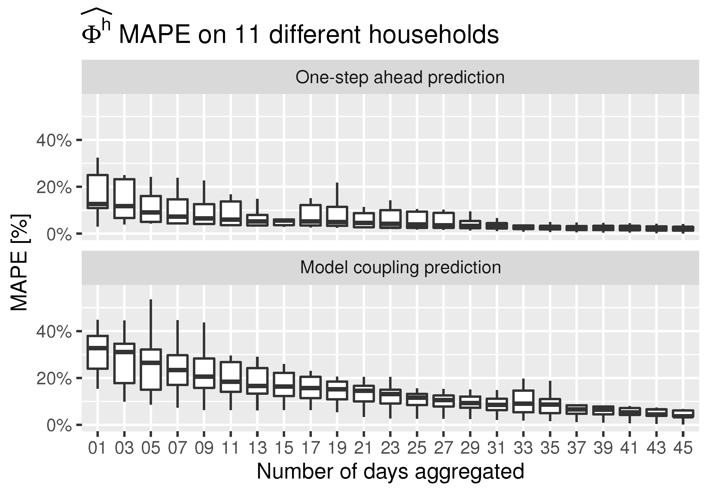
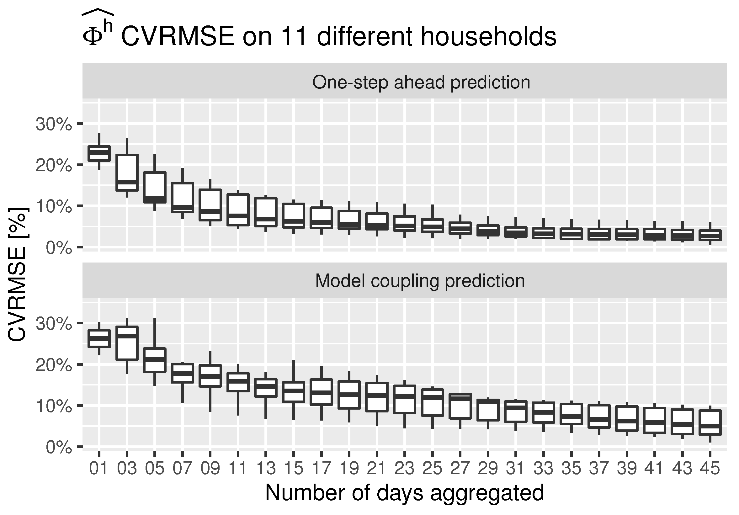
In Figure 11 and Figure 12, box-plots of the and for the space heating energy consumption are, respectively, shown for the 11 households, considering both prediction strategies and the same testing period. The is only computed when . As can be seen, the data are aggregated to several days to understand what the minimum period required to perform this kind of analysis is. In both, and , the errors evolved similarly, decreasing asymptotically as the aggregation frequency increased. When aggregation periods larger than 30 days are considered, both errors have an average value of less than 10%. Therefore, a minimum period of a month is recommended for the assessment of energy savings scenarios. It can also be concluded that both models are able to correctly characterize the dynamics of households since the error propagation does not increase sharply between both prediction strategies.
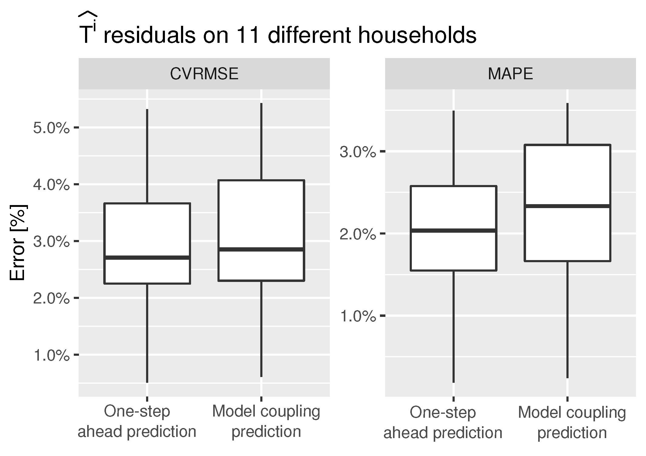
The box-plots of the and the , of the indoor temperature, are shown in Figure 13. The high accuracy of the demand-side model results in a very well predicted indoor temperature using both strategies. The hourly frequency residuals are lower than 3% on average. This means that the model is capable of accurately modeling the dynamics of the thermal losses and heat gains. This is of high importance since the indoor temperature is the variable used to control the operation of the space heating system of the households.
4.3. Assessment of Potential Energy Savings
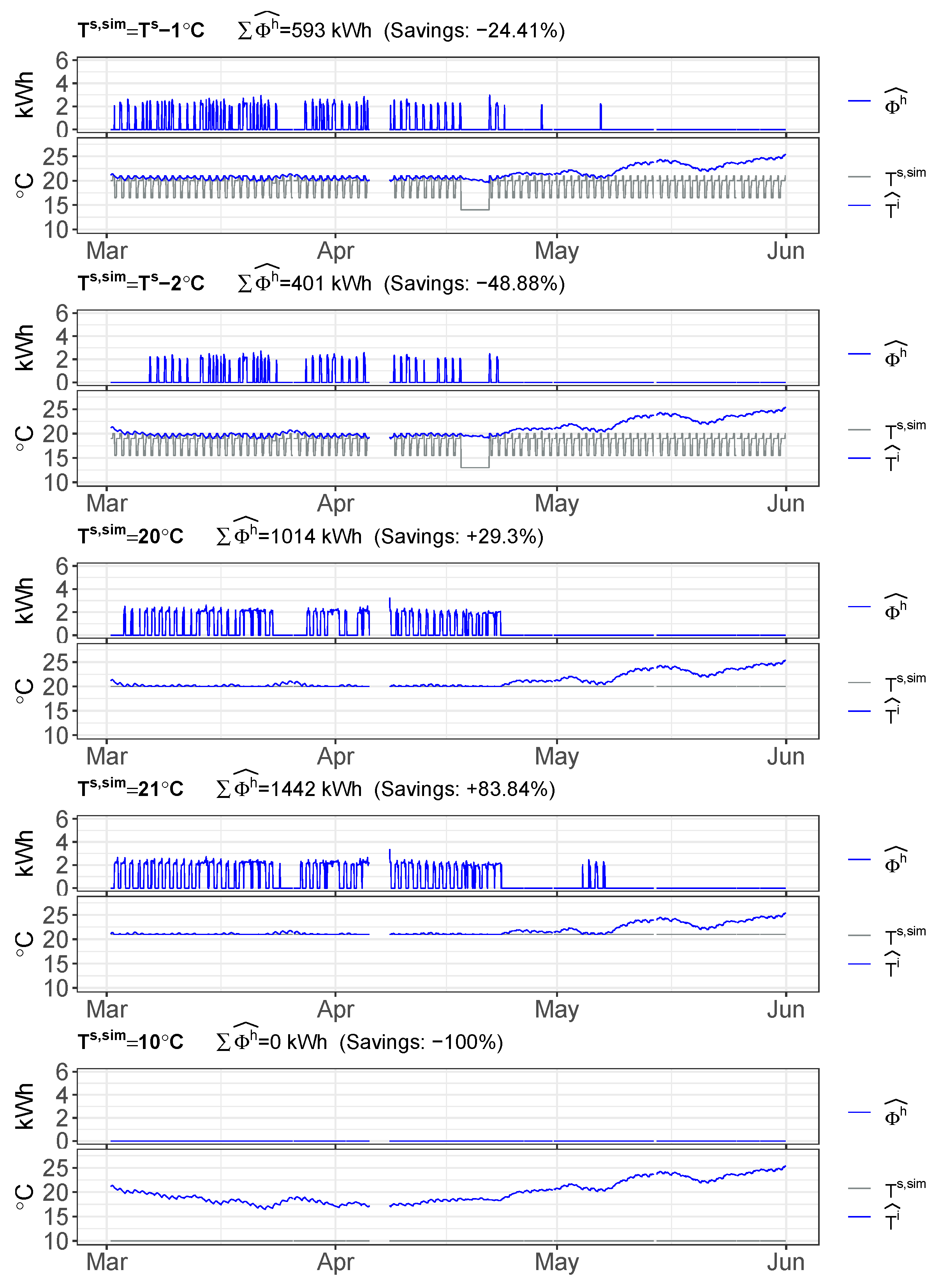
To envisage a wider applicability of the data-driven techniques developed in this research, the potential energy savings of several set point temperature scenarios over the analyzed household of Figure 5 are shown in Figure 14. As can be seen, in the period between 1st March and 31st May, the space heating energy consumption is estimated to decrease around 24% if the BaU set point schedule is lowered by 1 °C. If this BaU schedule is lowered by 2 °C, the estimated space heating energy savings reaches around 49%. These figures should be considered as approximate since the supply model has a higher error validation than the demand side model.
This data-driven methodology also allows the assessment of the response of the space heating energy consumption to time fixed values of the indoor temperature, as recommended by the building code regulations. Two predictions of fixed set point temperatures of 20 °C and 21 °C are generated and shown in the last top down plots of Figure 14. Although some level of energy savings was expected, the outcomes of these simulations yielded approximate energy consumption increases of around 29% and 84%, respectively. Therefore, for this household, it is not recommended to fix the temperature along the whole period, since this would lead to higher space heating energy consumption. This conclusion is in line with the set point temperature schedules set by the user in the BaU scenario, where 30 to 40% of the hours are set to low set point temperature. These low set point temperature periods correspond to the night time, when no energy gains are present and the outdoor temperatures are lower. In other words, even in case the values of the fixed set point temperature scenarios are lower than the higher values of the set point temperatures in the BaU scenario, the energy demand of the household increases to avoid the drop in the indoor temperature during this non-operational period.
Finally, the free-floating conditions can be also assessed. This facilitates the estimation of the minimum indoor temperature that a household would reach without the operation of the space heating system. In this case, this household would reach a minimum temperature of 16.7 °C along the whole tested period.
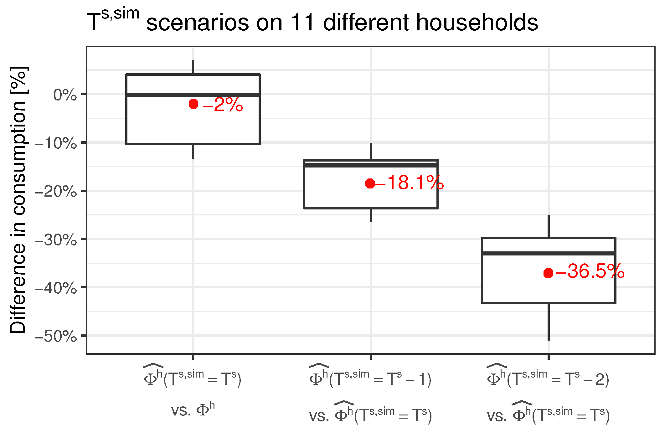
An assessment of approximate potential energy savings of the 11 households was performed. Figure 15 presents the box-plot of the energy consumption difference between the measured data and the simulated space heating energy consumption over the period between 1st March and 31st May. The first column represents the measured space heating energy consumption versus the predicted one, obtained by applying the Algorithm A1 considering the BaU set point temperature. The average difference is −2%, with an interquartile range between 4 and −10%. Since the absolute error is lower than 10%, it can be concluded that the trained models for the 11 households are valid to simulate set point temperatures scenarios. In the second and third columns, the comparison between two set point temperatures scenarios and the BaU set point temperature scenario is shown. Decreases of 1 °C and 2 °C are tested, yielding potential average energy savings of 18.1 and 36.5%, respectively.
5. Conclusions
The present research developed and validated a methodology to virtually emulate the performance of thermostatic load controlled systems relying on statistical learning models derived from the information gathered by smart thermostats. Two regression based models are developed: one with the supplied energy as the dependent variable (supply-side model), and another one with the indoor temperature as the dependent variable (demand-side model). Multiple exogenous variables, such as outdoor temperature, solar radiation, wind speed and wind direction are considered in addition to multiple input transformation techniques which enhance the accuracy of these models. A control algorithm, driven by the set point temperature, is implemented to couple both models and to be able to estimate the energy consumption and the indoor temperature when several set point temperature schedules are applied.
The methodology is validated in real cases within the winter season. One of the first findings is that the methodology used to train and couple the models, as well as the thermostatic control emulation, can be fully applicable to any space heating or cooling system as long as it is thermostatically controlled and a minimum historical data period is available. The study demonstrates a high accuracy of the models to predict both the indoor temperature and the space heating energy consumption. However, for this specific use case, since the measurement tolerance for the space heating consumption is too high, a minimum aggregated period of 30 days is recommended to properly estimate the potential energy savings scenarios. The novelty of the proposed methodology is that it goes beyond the prediction of the heat consumption and the of indoor temperature of these systems. The methodology incorporates an optimization algorithm and a control loop which provides the capability to virtually mimic all the possible user controlled modes driven by the set point temperature.
Another important finding of this research is that free-floating conditions of the analyzed households can also be assessed accurately. This gives the opportunity, for instance, to estimate, in the winter season, the lower indoor temperature that a household would reach without the operation of the space heating system.
A limitation of this methodology is related to data quality requirements when the models are trained. In this training period, the set point temperatures of the buildings need to be excited in the range of evaluation of the set point temperature scenarios. This excitation generates dynamic changes in indoor temperature and heat consumption that are subsequently inferred by the data-driven models. That means that a minimum period of historical data of set point temperatures within the range of normal operation, of indoor temperatures and of the space heating consumption, are required
Some direct conclusions can be finally obtained in relation to the potential energy savings which can be achieved if the users decide to modify their usual set point temperature schedule. Average estimated energy savings of 18.1% can be achieved if the usual set point temperature is lowered by 1 °C. Up to approximately 36.5% energy savings can be achieved if the usual set point temperature is lowered by 2 °C.
A further potential application of this research would be the use of this methodology as a forecasting toolbox for the short-term prediction of the impact, over the energy consumption and the indoor thermal conditions, of several set point temperature scenarios. For instance, this methodology could be used as a part of a Model Predictive Control (MPC) strategy aiming at minimizing the electricity cost of thermostatically controlled heat pumps due to market signals or at increasing the benefit of on-site renewable energy production (e.g., PV panels) while maintaining indoor comfort.
Author Contributions
Conceptualization, G.M., J.C. and D.C.; data curation, G.M. and B.G.; formal analysis, G.M. and E.G.; funding acquisition, J.C. and M.T.; investigation, G.M.; methodology, G.M. and B.G.; project administration, J.C. and M.T.; resources, M.T.; software, E.G.; supervision, J.C. and D.C.; validation, G.M.; writing—original draft, G.M.; writing—review and editing, J.C. and D.C. All authors have read and agreed to the published version of the manuscript.
Funding
This research received no external funding.
Institutional Review Board Statement
Not applicable.
Informed Consent Statement
Written informed consent was obtained from all subjects involved in the study.
Acknowledgments
We thank all the BAXI employees who provided insights and expertise that greatly assisted the work, and all their clients that participated in the project. D. Chemisana thanks ICREA for the ICREA Acadèmia. J. Cipriano thanks the Ministerio de Ciencia e Innnovacón for the Juan de la Cierva Incorporación grant.
Conflicts of Interest
The authors declare no conflict of interest.
Nomenclature
| Advanced Metering Infrastructure | |
| Artificial Neural Network | |
| American Society of Heating, Refrigerating and Air-Conditioning Engineers | |
| AutoRegressive Moving Average with eXogenous | |
| AutoRegressive with eXogenous | |
| Business as Usual | |
| Building Energy Simulation | |
| Coefficient of Variation of the Root Mean Squared Error | |
| Energy Conservation Measures | |
| European Union | |
| Heating, ventilation and air conditioning | |
| Internet of Things | |
| Information Technology | |
| Low-Pass Filter function | |
| Mean Absolute Percentage Error | |
| Non Linear Mixed Effect | |
| Resistor and Capacitor | |
| Root Mean Squared Error | |
| Space Heating | |
| Support Vector Machines | |
| Time Series |
Appendix A
| Algorithm A1. Forecasting algorithm and coupling of supply-side and demandside models | |
| Input: | Trained supply-side model; trained demand-side model; autoregressive orders , , , , , , , ; number of harmonics , and ; the smoothing parameters of the low-pass filter , and ; initial indoor conditions (), weather conditions during the whole evaluation period (outdoor temperature , wind speed , wind direction , solar irradiance , and solar position , ), the space heating consumption few timesteps before the period to be evaluated the hysteresis of the thermostat h and, finally, the setpoint temperature () to apply during the evaluation period |
| Output: | The predicted heat consumption () and the predicted indoor temperature () considering a setpoint temperature schedule () during a period . |
 | |

Table A1.
Columns of A matrix.
| Column | Conditions | Column | Conditions |
|---|---|---|---|
| - | |||
| - | - |
| Algorithm A2: Genetic Algorithm for the optimization of the auto regressive orders (), the low-pass filter (), and the number of harmonics () to be considered in the transformation of the input variables | |
| Input: Hourly space heating consumption, indoor and set point temperature of the thermostat and historical weather of the location of the household during a period where the boiler is operating. At least 3 months of data are required. | |
| Output: Find the optimal auto regressive orders , , , , , , , ; optimal number of harmonics , and ; and optimal smoothing parameters of the low-pass filter , and | |
|
DEFINE a test set and a training set (15% and 85%, respectively); DEFINE a cross-validation with 8 folds from the training set. Randomly select, for each of the folds, a set of 80% of the days for training and 20% for validation; SET the value ranges, levels and type of variables of the parameters to optimize; DEFINE an encode–decode technique to convert each single combination of parameters to a Reflected Binary Code (RBC) representation, taking into account the allowed ranges or levels assigned to each parameter; INITIALIZE population with random candidate RBC representations, also called chromosomes; EVALUATE the related cost of each chromosome using Algorithm A3. In this step, , , and ARX-models coefficients are estimated using the least squares method; | |
 | |
| Algorithm A3: Cost evaluation of each chromosome |
| Input: A chromosome which contains an RBC representation; training set; test set; and the description of the cross-validation folds. |
| Output: The cost related to the input chromosome |
 |
References
- Eurostat. Statistics Explained. Energy Consumption in Households. Technical Report. 2021. Available online: https://ec.europa.eu/eurostat/statistics-explained/index.php?title=Energy_consumption_in_households (accessed on 25 July 2021).
- Publications Office of the European Union. Clean Energy for All Europeans; Publications Office of the European Union: Luxembourg, 2019.
- Stafford, A. An exploration of load-shifting potential in real in-situ heat-pump/gas-boiler hybrid systems. Build. Serv. Eng. Res. Technol. 2017, 38, 450–460. [Google Scholar] [CrossRef]
- Rivoire, M.; Casasso, A.; Piga, B.; Sethi, R. Assessment of Energetic, Economic and Environmental Performance of Ground-Coupled Heat Pumps. Energies 2018, 11, 1941. [Google Scholar] [CrossRef] [Green Version]
- Zhang, X.; Strbac, G.; Teng, F.; Djapic, P. Economic assessment of alternative heat decarbonisation strategies through coordinated operation with electricity system—UK case study. Appl. Energy 2018, 222, 79–91. [Google Scholar] [CrossRef]
- Clegg, S.; Mancarella, P. Integrated electricity-heat-gas modelling and assessment, with applications to the Great Britain system. Part II: Transmission network analysis and low carbon technology and resilience case studies. Energy 2018, 184, 191–203. [Google Scholar] [CrossRef] [Green Version]
- Jarre, M.; Noussan, M.; Poggio, A.; Simonetti, M. Opportunities for heat pumps adoption in existing buildings: Real-data analysis and numerical simulation. Energy Procedia 2017, 134, 499–507. [Google Scholar] [CrossRef] [Green Version]
- European Commission—COM(2014) 356 Final. Benchmarking Smart Metering Deployment in the EU-27 with a Focus on Electricity 2014. Available online: https://ses.jrc.ec.europa.eu/publications/reports/benchmarking-smart-metering-deployment-eu-27-focus-electricity (accessed on 24 August 2021).
- Farhangi, H. The path of the smart grid. IEEE Power Energy Mag. 2010, 8, 18–28. [Google Scholar] [CrossRef]
- Newe, G. Delivering the Internet of Things. Netw. Secur. 2015, 2015, 18–20. [Google Scholar] [CrossRef]
- Pritoni, M.; Meier, A.K.; Aragon, C.; Perry, D.; Peffer, T. Energy efficiency and the misuse of programmable thermostats: The effectiveness of crowdsourcing for understanding household behavior. Energy Res. Soc. Sci. 2015, 8, 190–197. [Google Scholar] [CrossRef] [Green Version]
- Peffer, T.; Pritoni, M.; Meier, A.; Aragon, C.; Perry, D. How people use thermostats in homes: A review. Build. Environ. 2011, 46, 2529–2541. [Google Scholar] [CrossRef] [Green Version]
- Apex Analytics LLC. Energy Trust of Oregon Smart Thermostat Pilot Evaluation; Apex Analytics LLC: Boulder, CO, USA, 2016; p. 152. [Google Scholar]
- Koupaei, D.M.; Song, T.; Cetin, K.S.; Im, J. An assessment of opinions and perceptions of smart thermostats using aspect-based sentiment analysis of online reviews. Build. Environ. 2020, 170, 106603. [Google Scholar] [CrossRef]
- Huchuk, B.; O’Brien, W.; Sanner, S. A longitudinal study of thermostat behaviors based on climate, seasonal, and energy price considerations using connected thermostat data. Build. Environ. 2018, 139, 199–210. [Google Scholar] [CrossRef]
- Stopps, H.; Touchie, M.F. Managing thermal comfort in contemporary high-rise residential buildings: Using smart thermostats and surveys to identify energy efficiency and comfort opportunities. Build. Environ. 2020, 173, 106748. [Google Scholar] [CrossRef]
- Huchuk, B.; Sanner, S.; O’Brien, W. Comparison of machine learning models for occupancy prediction in residential buildings using connected thermostat data. Build. Environ. 2019, 160, 106177. [Google Scholar] [CrossRef]
- Parker, D.; Sutherland, K.; Chasar, D. Evaluation of the Space Heating and Cooling Energy Savings of Smart Thermostats in a Hot-Humid Climate using Long-term Data. ACEEE Summer Study Energy Eff. Build. 2016, 2016, 15. [Google Scholar]
- Pritoni, M.; Woolley, J.M.; Modera, M.P. Do occupancy-responsive learning thermostats save energy? A field study in university residence halls. Energy Build. 2016, 127, 469–478. [Google Scholar] [CrossRef]
- Stopps, H.; Touchie, M.F. Reduction of HVAC system runtime due to occupancy-controlled smart thermostats in contemporary multi-unit residential building suites. IOP Conf. Ser. Mater. Sci. Eng. 2019, 609, 062013. [Google Scholar] [CrossRef] [Green Version]
- Manning, M.; Swinton, M.; Szadkowski, F.; Gusdorf, J.; Ruest, K. The effects of thermostat setback and setup on seasonal energy consumption, surface temperatures, and recovery times at the CCHT twin house research facility. ASHRAE Trans. 2007, 113, 630–641. [Google Scholar]
- Soldo, B. Forecasting natural gas consumption. Appl. Energy 2012, 92, 26–37. [Google Scholar] [CrossRef]
- Tavakoli, E.; Montazerin, N. Stochastic analysis of natural gas consumption in residential and commercial buildings. Energy Build. 2011, 43, 2289–2297. [Google Scholar] [CrossRef]
- Diao, L.; Sun, Y.; Chen, Z.; Chen, J. Modeling energy consumption in residential buildings: A bottom-up analysis based on occupant behavior pattern clustering and stochastic simulation. Energy Build. 2017, 147, 47–66. [Google Scholar] [CrossRef]
- Brabec, M.; Konár, O.; Pelikán, E.; Malý, M. A nonlinear mixed effects model for the prediction of natural gas consumption by individual customers. Int. J. Forecast. 2008, 24, 659–678. [Google Scholar] [CrossRef]
- Soldo, B.; Potočnik, P.; Simunovic, G.; Saric, T.; Govekar, E. Improving the residential natural gas consumption forecasting models by using solar radiation. Energy Build. 2014, 69, 498–506. [Google Scholar] [CrossRef]
- Li, W.; Tian, Z.; Lu, Y.; Fu, F. Stepwise calibration for residential building thermal performance model using hourly heat consumption data. Energy Build. 2018, 181, 10–25. [Google Scholar] [CrossRef]
- Wang, J.; Tang, C.Y.; Brambley, M.R.; Song, L. Predicting home thermal dynamics using a reduced-order model and automated real-time parameter estimation. Energy Build. 2019, 198, 305–317. [Google Scholar] [CrossRef]
- Aliberti, A.; Bottaccioli, L.; Macii, E.; Di Cataldo, S.; Acquaviva, A.; Patti, E. A Non-Linear Autoregressive Model for Indoor Air-Temperature Predictions in Smart Buildings. Electronics 2019, 8, 979. [Google Scholar] [CrossRef] [Green Version]
- Alanezi, A.; Hallinan, K.P.; Elhashmi, R. Using Smart-WiFi Thermostat Data to Improve Prediction of Residential Energy Consumption and Estimation of Savings. Energies 2021, 14, 187. [Google Scholar] [CrossRef]
- Trovato, V.; De Paola, A.; Strbac, G. Distributed Control of Clustered Populations of Thermostatic Loads in Multi-Area Systems: A Mean Field Game Approach. Energies 2020, 13, 6483. [Google Scholar] [CrossRef]
- Doğan, A.; Alçı, M. Real-time demand response of thermostatic load with active control. Electr. Eng. 2018, 100, 2649–2658. [Google Scholar] [CrossRef]
- Nielsen, H.A.; Madsen, H. Modelling the heat consumption in district heating systems using a grey-box approach. Energy Build. 2006, 38, 63–71. [Google Scholar] [CrossRef] [Green Version]
- Bacher, P.; Madsen, H.; Nielsen, H.A.; Perers, B. Short-term heat load forecasting for single family houses. Energy Build. 2013, 65, 101–112. [Google Scholar] [CrossRef] [Green Version]
- Scrucca, L. GA: A Package for Genetic Algorithms in R. J. Stat. Softw. 2013, 53, 1–37. [Google Scholar] [CrossRef] [Green Version]
- Scrucca, L. On Some Extensions to GA Package: Hybrid Optimisation, Parallelisation and Islands EvolutionOn some extensions to GA package: Hybrid optimisation, parallelisation and islands evolution. R J. 2017, 9, 187–206. [Google Scholar] [CrossRef] [Green Version]
- Mor, G.; Vilaplana, J.; Danov, S.; Cipriano, J.; Solsona, F.; Chemisana, D. EMPOWERING, a Smart Big Data Framework for Sustainable Electricity Suppliers. IEEE Access 2018, 6, 71132–71142. [Google Scholar] [CrossRef]
- Dark sky Web Service, Dark Sky. 2021. Available online: https://darksky.net/dev (accessed on 25 July 2021).
- Council of the European Union, European Parliament. Regulation (EU) No. 377/2014 of the European Parliament and of the Council of 3 April 2014 Establishing the Copernicus Programme and repealing Regulation (EU) No 911/2010 Text with EEA Relevance. 2014. Available online: https://eur-lex.europa.eu/legal-content/EN/TXT/HTML/?uri=CELEX:32014R0377&from=EN (accessed on 25 July 2021).
Figure 1.
General steps and objectives of the modeling technique presented.

Figure 2.
Theoretical examples of 3 different set point temperatures scenarios over the same time period and their related indoor temperature and space heating consumption.
Figure 2.
Theoretical examples of 3 different set point temperatures scenarios over the same time period and their related indoor temperature and space heating consumption.

Figure 3.
Models coupling flow diagram.

Figure 4.
Pictures of the installation of the smart thermostat (BAXI CONNECT) in one of the case study households. The top row shows the removal of the front cover of the boiler. The middle row shows the connection with the gateway. The bottom row shows the new smart thermostat installation.
Figure 4.
Pictures of the installation of the smart thermostat (BAXI CONNECT) in one of the case study households. The top row shows the removal of the front cover of the boiler. The middle row shows the connection with the gateway. The bottom row shows the new smart thermostat installation.

Figure 5.
Input and output variables of the demand and supply-side models for one household.

Figure 6.
Actual set point and indoor temperature for one household.

Figure 7.
Training residuals of the model with as output.

Figure 8.
The 20 levels for a float parameter () considering a uniform or an exponential weight distribution.
Figure 8.
The 20 levels for a float parameter () considering a uniform or an exponential weight distribution.

Figure 9.
Training residuals of the model with as output.

Figure 10.
Accuracy of and forecasting from 1st March to 31st May using Algorithm A1 and considering the real set point temperature (). The cumulative consumption over the period is: kWh kWh).
Figure 10.
Accuracy of and forecasting from 1st March to 31st May using Algorithm A1 and considering the real set point temperature (). The cumulative consumption over the period is: kWh kWh).

Figure 11.
MAPE of the space heating consumption of 11 households, aggregating data to daily multiples.
Figure 11.
MAPE of the space heating consumption of 11 households, aggregating data to daily multiples.

Figure 12.
CVRMSE of the space heating consumption of 11 households aggregating data to daily multiples.
Figure 12.
CVRMSE of the space heating consumption of 11 households aggregating data to daily multiples.

Figure 13.
Hourly indoor temperature CVRMSE and MAPE of 11 households.

Figure 14.
Energy potential savings applying different set point temperatures scenarios () over one household.
Figure 14.
Energy potential savings applying different set point temperatures scenarios () over one household.

Figure 15.
Energy potential savings distributions applying two different set point temperatures scenarios () over 11 households.
Figure 15.
Energy potential savings distributions applying two different set point temperatures scenarios () over 11 households.

Table 1.
Model coefficients configuration for each exogenous variable.
| Parameter | Type | Values Range | Number of Levels | Weights Distribution * | Optimal Value for Household in Study |
|---|---|---|---|---|---|
| integer | 4 | uniform | 1 | ||
| integer | 8 | uniform | 5 | ||
| integer | 4 | uniform | 3 | ||
| integer | 4 | uniform | 0 | ||
| integer | 16 | uniform | 13 | ||
| integer | 4 | uniform | 1 | ||
| integer | 4 | uniform | 1 | ||
| integer | 4 | uniform | 0 | ||
| integer | 3 | uniform | 2 | ||
| integer | 3 | uniform | 1 | ||
| integer | 3 | uniform | 1 | ||
| float | 20 | exponential | 0.891 | ||
| float | 14 | exponential | 0.252 | ||
| float | 18 | exponential | 0.824 | ||
| discrete | ** | 3 | uniform | linear depending solar position | |
| discrete | *** | 3 | uniform | linear depending wind direction | |
| h | float | 4 | uniform | 0.5 |
Notes: * see Figure 8; ** no dependence, linear dependence, and linear depending solar position; *** no dependence, linear dependence, and linear depending wind direction.
Publisher’s Note: MDPI stays neutral with regard to jurisdictional claims in published maps and institutional affiliations. |
© 2021 by the authors. Licensee MDPI, Basel, Switzerland. This article is an open access article distributed under the terms and conditions of the Creative Commons Attribution (CC BY) license (https://creativecommons.org/licenses/by/4.0/).
Share and Cite
MDPI and ACS Style
Mor, G.; Cipriano, J.; Gabaldon, E.; Grillone, B.; Tur, M.; Chemisana, D. Data-Driven Virtual Replication of Thermostatically Controlled Domestic Heating Systems. Energies 2021, 14, 5430. https://doi.org/10.3390/en14175430
AMA Style
Mor G, Cipriano J, Gabaldon E, Grillone B, Tur M, Chemisana D. Data-Driven Virtual Replication of Thermostatically Controlled Domestic Heating Systems. Energies. 2021; 14(17):5430. https://doi.org/10.3390/en14175430
Chicago/Turabian StyleMor, Gerard, Jordi Cipriano, Eloi Gabaldon, Benedetto Grillone, Mariano Tur, and Daniel Chemisana. 2021. "Data-Driven Virtual Replication of Thermostatically Controlled Domestic Heating Systems" Energies 14, no. 17: 5430. https://doi.org/10.3390/en14175430
Note that from the first issue of 2016, this journal uses article numbers instead of page numbers. See further details here.