Application of Ordinal Optimization to Reactive Volt-Ampere Sources Planning Problems


1
Department of Computer Science & Information Engineering, Yuan Ze University, Taoyuan City 32003, Taiwan
2
Department of Computer Science & Information Engineering, Chaoyang University of Technology, Taichung City 41349, Taiwan
*
Author to whom correspondence should be addressed.
Energies 2019, 12(14), 2746; https://doi.org/10.3390/en12142746
Submission received: 2 July 2019
/
Revised: 15 July 2019
/
Accepted: 16 July 2019
/
Published: 17 July 2019
(This article belongs to the Special Issue Electric Power Systems Research 2019)
Abstract
:Reactive volt-ampere sources planning is an effort to determine the most effective investment plan for new reactive sources at given load buses while ensuring appropriate voltage profile and satisfying operational constraints. Optimization of reactive volt-ampere sources planning is not only a difficult problem in power systems, but also a large-dimension constrained optimization problem. In this paper, an ordinal optimization-based approach containing upper and lower level is developed to solve this problem efficiently. In the upper level, an ordinal search (OS) algorithm is utilized to select excellent designs from a candidate-design set according to the system’s structural information exploited from the simulations executed in the lower level. There are five stages in the ordinal search algorithm, which gradually narrow the design space to search for a good capacitor placement pattern. The IEEE 118-bus and IEEE 244-bus systems with four load cases are employed as the test examples. The proposed approach is compared with two competing methods; the genetic algorithm and Tabu search, and a commercial numerical libraries (NL) mixed integer programming tool; IMSL Numerical Libraries. Experimental results illustrate that the proposed approach yields an outstanding design with a higher quality and efficiency for solving reactive volt-ampere sources planning problem.
1. Introduction
Reactive volt-ampere sources planning is an effort to determine the most effective investment plan for new reactive sources at given load buses while ensuring appropriate voltage profile and satisfying operational constraints [1,2]. Reactive volt-ampere source planning has been studied without paying much consideration to the time-varying characteristic of reactive power. In general, resource and transmission planners adopt a classical power factor band for the reactive power flow at grid interface points and focus on future active power demand using conventional load forecasts. Optimization of reactive volt-ampere sources planning involves optimizing the sizes of the switchable capacitors and allocation optimization. The goal of this problem is decreasing the system real losses, improving the voltage profile, and achieving the reactive power demand when the system expands. Common objective functions include the cost of the installed reactive power sources and overall system’s real losses. The switchable capacitor bank plays a crucial role in the reactive power demand, since it adjusts the reactive power injection for maintaining the local voltage profile under different loading conditions. Most power networks are public facilities, and their investment budgets need approval from the Congress. However, unavoidable budget cuts occur frequently. The reactive power installation cost is served as the objective value, and it is also regarded as an investment constraint to extract the whole available budget. Thus, the goal is to minimize the weighted sum of system losses for different loading cases subject to the following four constraints: (i) switchable capacitor constraints, (ii) investment constraints on reactive power sources of switchable capacitor banks, (iii) security constraints of all load cases, and (iv) power flow balance equations.
The considered problem is difficult to solve because the allocation and sizes of the capacitor placement are integer and discrete values, respectively. A variety of methods have been successfully employed for solving this kind of problem [3,4,5,6,7,8]. In most existing methods, the exact form does not consider the integer and discrete variables simultaneously. With the advancements in computational technologies, optimization methods including the meta-heuristic [9], swarm intelligence [10] and direct search method [11], which was developed for solving the recent reactive volt-ampere sources planning problems. Although these methods are able to handle integer, discrete and continuous variables, they are often time-consuming. Simulation optimization technique is an alternative to solve the considered problem. Simulation optimization is frequently used for searching the optimal input setting to optimize the output performance of a simulated system [12,13]. Zhu et al. proposed a mixed-integer particle swarm optimization algorithm on optimal placement of battery energy storage systems to improve power system oscillation damping, in which the New England 39-bus system and the Nordic test system were used as test examples [14]. Abdelaziz and Moradzadeh presented a parallelized implementation of NSGA-II using OpenCL to solve the multi-objective renewable DG planning problem, where the IEEE 32-bus test system and two real distribution test systems were used as test examples [15]. Roberts et al. proposed a probabilistic simulation-based multi-objective optimization approach for dimensioning robust renewable based Hybrid Power Systems, where a rural community of the Amazonian region of Brazil was used as a test example [16]. Ebrahimzadeh et al. presented a multi-objective optimization procedure based on the genetic algorithm to decide optimum design of power converter current controllers in power electronics-based systems, where a 400-MW wind farm with 100-MW aggregated strings was used as a test example [17].
We adopt the framework of simulation optimization to the reactive volt-ampere sources planning problem by two mappings: (i) the pattern of capacitor placement is regarded as an input setting; and (ii) the weighted sum of system losses for various load cases is regarded as the output performance. The framework of the proposed ordinal optimization-based approach is shown in Figure 1. The performance of a real system can be approximated as an output of the computer simulation by solving an optimal power flow (OPF)-like problem. However, the considered problem with both continues, and discrete variables belong to a type of NP-complete optimization problems due to the huge design space of the discrete control variables setting. Accordingly, it is much more difficult to solve the mixed continuous and discrete control variables optimization problems within a reasonable computation time. In addition, solving a large-scale OPF-like problem is very time-consuming because a lengthy simulation is used to evaluate the performance of a design. To overcome this drawback, an ordinal optimization-based approach containing upper and lower level is proposed for solving the reactive volt-ampere sources planning problems. An ordinal search (OS) algorithm is adopted as an optimization technique in the upper level, and a dual-type method [18,19,20] is used as the simulation tool in the lower level to solve the large-scale OPF-like problems.
There are five stages in the proposed OS algorithm, whose basic idea is to perform ranking and selection at each stage. A design vector contains all bus complex voltages, real and reactive power generations, load demands and the transformer tap ratios of all load cases. A feasible design vector must satisfy the following four constraints: switchable capacitor constraints, investment constraints on reactive power sources of switchable capacitor banks, security constraints of all load cases, and power flow balance equations. Efficiently ranking the designs in the candidate-design set at every stage is based on a model constructed by the system’s structural information exploited from the simulations. The selected excellent designs will construct the reduced candidate-design set for next stage. The OS algorithm is adopted to solve for a superior design at the last stage. The advantage of the proposed method is to reduce the required simulation time dramatically by concentrating on finding good enough designs instead of insisting on picking the best design. However, obtaining a good enough subset of designs may not be very satisfactory in some cases. The disadvantage of the proposed method is that it does not offer an absolute guarantee of the global optimality.
The first contribution of this research is to develop a simulation model for reactive volt-ampere sources planning problems, which is mapping to an optimal power flow (OPF)-like problem. The second contribution is to propose an ordinal optimization-based approach for solving the OPF-like problem, in order to determine an outstanding design in a short computational time. The third contribution is to employ the proposed approach for three network configurations with one outage, two outages and three outages in heavily load cases.
The organization of this paper is as follows. Section 2 introduces the considered problem and describes the mathematical formulation of the reactive volt-ampere sources planning with multiple load cases. Section 3 presents the OS five stages approach. In Section 4, the IEEE 118-bus and IEEE 244-bus systems are used as the examples to test the proposed ordinal optimization-based approach. We also compare the computational performance and the design quality with two competing algorithms, genetic algorithm (GA) and Tabu search (TS), and a commercial numerical libraries (NL) mixed integer programming routine, IMSL Numerical Libraries. Finally, Section 5 draws a brief conclusion.
2. Mathematical Formulation
The reactive volt-ampere sources planning problem belongs to a class of constrained multi-objective optimization problems. Objective functions utilized in this problem are usually due to the overall system’s real losses, the cost of the installed reactive power sources, or both [21,22]. In most countries, the power network is a public facility whose investment budget needs approval from the Congress. Most of the time, the overall investment budget is within a certain limit. Supposing that the cost of reactive volt-ampere sources placements is minimized; the installation cost will exceed the investment budget. Therefore, the sum of weighted system losses of various loading profiles is treated as an objective function. Meanwhile, the installation cost is treated as an investment constraint so as to exploit the entire available budget. Hence, the reactive volt-ampere sources planning problem can be formulated as follows.
where N is amount of load cases; denotes the design vector, which can be variable vector of all bus complex voltages, real and reactive power generations, load demands and the transformer tap ratios of the ith load case and are of the continuous variables; and represent the weighting factor and overall system losses of the ith load case, respectively; represents the flow balance equations of the ith load case; is the security constraints on real and reactive power generations, voltage magnitude, and real power line flow; J denotes the set of candidate buses to install switchable capacitors banks; is the switchable capacitor banks installing at bus w, , ; is the part of bus w’s in load case , , ; , if bus w is installed, then , else, ; qw is the cost per MVAR capacitance; qow is the installation cost at bus w; and M is the overall investment budget. The considered problem is difficult to solve because and belong to discrete variables while belong to integer variables.
3. Simulation Optimization
The key idea of the proposed OS algorithm is based on the ordinal optimization (OO) theory [23,24]. OO is not intended to replace the other optimization approaches. Instead, it is utilized to assist other optimization approaches. OO theory uses the term “order” rather than “value” to resolve the computing complexity, and provides a high probability guarantee to an outstanding design. In OO theory, a good enough or outstanding solution is defined as a solution that is among the top 3.5% of all solutions with a high probability of 0.95 [23]. This does not mean that a good enough solution is within 3.5% of the optimal cost. For many problems, a fairly large number of solutions perform close to the true optimum. In these cases, the qualitative difference among good enough polices is small and more than offset by the expense of trying to find the best solution. OO theory has been used extensively and successfully in some hard optimization problems, including network-type production line [25], flow line system [26], assemble-to-order systems [27] and pull-type production system [28].
3.1. Five Stages in the OS Algorithm
The five stages in the OS algorithm are stated below.
Stage (i): apply sensitivity theory for searching the effective locations to place capacitors.
The sensitivity theory is adopted to search for the effective locations among to place capacitors and decide . Firstly, every candidate bus in is installed with a settled 1-bank capacitor, and all components of in the flow balance equations are equal to 1. Note that the purpose of this fictitious assumption is to extract the structural information of the system to assist decision about the effective locations for placing capacitors. Thus, the investment constraint and the switchable capacitors constraint in (1) can be ignored, and problem (1) can be simplified as follows.
where denotes the capacitance vector of 1-bank capacitor at all buses . Thus, problem (2) can be solved by the lower level in Figure 1 so as to extract the structural information for the upper level, then the OS algorithm is used to select the effective locations. In addition, the dual-type method [18] is adopted as the simulation tool for solving (2).
Based on the sensitivity theory [29], the sensitivity of deviation for objective value of (2) caused by the increase on the capacitance is computed by , where denotes the optimal Lagrange multiplier vector of load case . If the value of is negative and large, then increasing will decrease the overall system losses. It means that bus has a stronger effect on lowering the objective function. Accordingly, sensitivity of cost reduction along with each candidate bus resulted from solving (2) will be provided to the upper level to rank the candidate buses in J. Details of the process are stated as follows.
First, all candidate buses are ranked according to the sensitivity values, i.e., . The smaller the sensitivity value, the higher the order. Let denote the ranked indices of , where denotes the amount of buses in (·). Thus, the bus is the highest order candidate bus. Starting from , we subtract the corresponding and from the ,. This subtraction is proceeded until all of the investment budget is exhausted. If the subtraction is terminated at the candidate buses , where , then construct the effective buses that allocate the switchable capacitors. Furthermore, can be partitioned into sets of effective candidate buses.
Stage (ii): search the refined locations through simulation and obtain the optimal continuous value of the capacitance.
In Stage (i), the sensitivity approach just roughly estimates the performance of locations for placing capacitors. In Stage (ii), a simulation approach is used to decide the refined ones from the candidate buses obtained in Stage (i). The value of for the refined locations is still one, while the remaining values are zero.
To achieve this target, the ready to place capacitors are assumed to be continuous values. Since there are many iterative processes between the upper level and lower level, we let in the beginning. is defined as the set of the refined candidate buses to install switchable capacitor banks obtained from Stage (ii). We then set , in the flow balance equations. After subtracting candidate buses in from , problem (1) can be reformulated as follows:
where and are assumed to be continuous, and .
Since problem (3) belongs to the simulation level, the dual-type method [18,19,20] is utilized for solving it. Once this issue has been resolved, the obtained optimal continuous values of are used to update and in the upper level. A small value of one-bank optimal continuous capacitance represents that it is ineffective to locate this capacitor. If there is any optimal continuous , which is less than the capacitance of one bank, this set of buses, say ’s, from will be discarded. Therefore, we can compute in (3) in the upper level. We can also calculate the value of in (3) by using the updated . This iterative process is repeated until the optimal value of capacitance in each bus is greater than or equal to 1-bank. The last represents the refined buses determined by Stage (ii). The value of , is still one, while the remaining values are zero. The obtained optimal continuous design of and , for (3) with the most updated and , are denoted by and , respectively, and the corresponding optimal are denoted as . We denote and as the optimal and vector of optimal Lagrange multiplier for the flow balance equations of the th load case in the continuous version of optimal capacitance value determination problem (3), respectively.
Stage (iii): choose the excellent discrete capacitors placement patterns using a rough model of (1).
Although the values of optimal and resulted from Stage (ii) are continuous, their adjacent discrete values may be viewed as good discrete designs. However, there are totally combinations of the adjacent discrete patterns for placing switchable capacitors. Let represent the th discrete pattern vector, , where , so that ⎡⎤ or , . However, merely the discrete patterns satisfying the investment constraint are feasible. Assuming there are feasible patterns satisfying the investment constraint, these patterns are denoted as . What needs to be further clarified is the part of utilized in load case , which will influence the value of . To assess the performance of a discrete pattern , we have to consider all the possible selections of switchable capacitors corresponding to that pattern and determine the one that can achieve the optimal objective value, which will be taken as the performance of the given . However, choosing the best is another combinatorial problem. Thus, we will determine an exceptional choice instead of the best as addressed in [20]. First, we evaluate the exceptional selections of for a given . Next, we calculate the minimal deviation concerning the objective value caused by the deviations of and from the optimal continuous values of and for (3). The detail processes are stated as follows.
(1) Evaluate the exceptional selections within for a given
Firstly, the discrete values for closest left and right side of are denoted as and , respectively. Consider a discrete capacitor placement pattern, , load case has at most exceptional selections of the adjacent discrete values of . We let represent the number of acceptable exceptional selections of for load case such that . Then, the total amount of exceptional selections of is . We let represent the th choice of , where . We define as the deviation of the th discrete capacitor from the optimal continuous , where . Details of the minimal deviations concerning the objective values of (3) caused by the total deviation for a given are stated below.
(2) Compute the minimal deviations concerning the objective value caused by all deviations .
Consider a given , the deviation concerning the objective value caused by all deviations of capacitance values , denoted by , is calculated by the sensitivity theory.
The minimization problem concerning the deviations caused by the is formulated as follows.
We define and denote the minimum objective value of (5) by .
Since no discrete pattern can achieve a better objective value than the optimal values of and , thus for any deviation . In fact, the smaller the is, the better the discrete pattern will be. Thus, by the aid of , we are ready to choose the top patterns.
(3) Choosing the top patterns.
The feasible patterns are ranked based on the from the smallest to the largest. The former patterns are selected as the excellent discrete capacitor placement patterns, which are denoted as . The corresponding switchable capacitors for load case , are denoted as .
Stage (iv): determine the top from the patterns using a quadratic approximation model of (1).
Suppose each candidate bus may install 1 to banks, the original candidate-design set will consist of patterns. Provided that and |J|=20, then . This means the size of the candidate-design set has reduced from to up to present stage. However, evaluating these patterns using an accurate model of (1) is still time-consuming. According to [20], a quadratic approximation model of (1) is used to assess these patterns, and the top , say 3, patterns would contain the superior design. Because the discrete patterns, , and the corresponding , resulted from Stage (iii) have satisfied the investment and switchable capacitors constraints, the following quadratic approximation model of (1) is adopted to assess the patterns.
where the switchable capacitors and ready to place capacitors for all load cases in (1) are settled at and , and the quadratic approximation is assessed at . The dual-type method proposed in [18,19,20] is used for solving (6), since the quadratic approximation model in (6) is a quadratic programming problem. Let represent the optimal design of (6), then is an approximate design of (1) under the given and the corresponding . Furthermore, denotes the corresponding approximate objective value. The top patterns with smaller approximate objective values are selected for next stage.
Stage (v): employ the accurate model to assess the patterns resulted from Stage (iv) and determine the superior design of (1).
The top k capacitors placement patterns selected in Stage (iv) are denoted as , whose switchable capacitors for load case are denoted as . Because the top discrete patterns and the corresponding have satisfied the investment and switchable capacitors constraints, the following accurate model of (1) is adopted to assess the patterns.
The dual-type method is employed for solving the OPF of multiple load cases shown in (7).
Let represent the optimal objective value of (7) for and . Let , thus is the superior capacitor placement pattern, and is the superior part of discrete switchable capacitors for load case .
3.2. Flow Diagram of the Ordinal Search (OS) Algorithm
4. Experiment Results
4.1. Test Examples and Results
The IEEE 118-bus and IEEE 244-bus systems with four load cases are employed as the test examples. The size of a bank was 14.4 MVAR. The upper limit of capacitor banks for capacitors was 3, which can be coded using two bits. The cost of installation and switchable capacitor bank were $1000 and $900 USD, respectively. There are five cases of investment budget, which are M = $40,000, $50,000, $60,000, $70,000 and $80,000 USD. The weighting factor was equal to 1 for load cases . The values of and in Stages (iii) and (iv) were set to be 35 and 3, respectively. The simulation experiment was coded in C++ in Microsoft Visual Studio 2013 and implemented on an Intel Core i7, 4.6 GHz CPU, 8 GB RAM desktop computer.
Table 1 and Table 2 show the simulation results of the superior capacitor placement patterns for five investment cases. Column 2 presents the actual amount of investment (installation costs). Columns 3 and 4 display the system losses and the consumed CPU time, respectively. Column 5 displays the number of candidate buses in resulted from Stage (ii) of the proposed approach. Figure 3 and Figure 4 display the objective value corresponding to the investment budget for five investment cases. The more the investment budget, the lower the real power loss. The reactive volt-ampere sources installing to the system not only compensate the reactive power, but also reduce the power losses. Test results of reactive volt-ampere locations and size on the IEEE 118-bus [30] and 244-bus systems [31] are shown in Table 3 and Table 4, respectively.
Test results further demonstrate that the proposed approach gradually narrows the design space to search for a good capacitor placement pattern. In addition, the random selection is used to select the candidate location on the same test system, whose results are also shown in Table 5 and Table 6. Test result without capacitors are also shown in Table 5 and Table 6. Column 4 shows the power loss reduced rates, and it reveals that the proposed approach yields a good capacitor placement pattern.
4.2. Comparison with the Competing Methods
To demonstrate the computing efficiency of the proposed method, two heuristic methods, GA and TS methods were utilized to solve the IEEE 118-bus system under the same five investment cases.
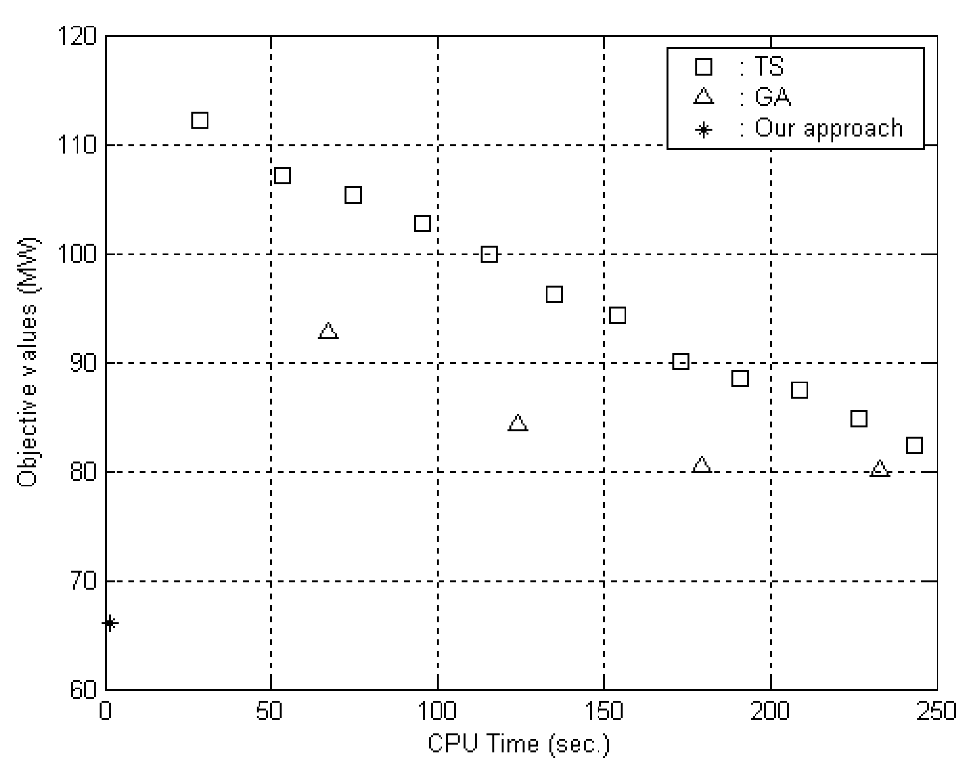
In the GA, a binary coding scheme was used to express the feasible capacitors placement patterns and the related switchable capacitors used in all load cases. The population size was 30. Roulette wheel selection was employed to select parents from mating pool for crossover. A two-point crossover with a crossover rate 0.7 was utilized, and the generated offspring will replace the parents in the mating pool. A mutation with rate 0.02 was performed on each resulted individual in the mating pool [32]. The fitness of each individual was evaluated by the dual-type method for solving the continuous OPF of multiple load cases. The points marked by “Δ” in Figure 5 represent the progression of the best-so-far objective values versus the consumed CPU time for the GA applied to the investment case 1. The point marked by “∗” represents the objective value and the consumed CPU times resulted from the proposed approach. GA consumed about 150 times of the CPU time consumed by the proposed approach, whose corresponding best-so-far objective value was 21% more than our approach. In Figure 5, the points marked by “□” represent the progression of the best-so-far objective value versus the consumed CPU time for the TS. When the TS consumed about 150 times of the CPU time consumed by the proposed approach, its best-so-far objective value is still 32% more than our approach.
The remainder of the four investment cases were also tested using both methods with the dual-type method. They were terminated when they consumed around 150 times of the CPU time consumed by the proposed approach. Experiment results are shown in Table 7 and Table 8, respectively. The percentages of objective value reduction are shown in columns 4 of Table 7 and Table 8. Accordingly, the computational efficiency and objective reduction are significance of the proposed method with respect to the two heuristic methods, GA and TS, which were utilized to solve the IEEE 118-bus system under the same five investment cases.
Finally, with an existing benchmark commercial NL mixed integer programming tool, we compared the International Mathematics and Statistics Library (IMSL) Numerical Libraries [33]. The IMSL C Numerical Library 2016.1 was utilized to solve the same investment cases on the seven IEEE systems, which are the IEEE 6-bus, 9-bus, 11-bus, 30-bus, 57-bus, 118-bus and 244-bus systems. Test results are shown in Table 9. No result is obtained with the IMSL for the IEEE 118-bus and 244-bus system because of the large memory requirement. The proposed approach is 84.21 times faster than IMSL for the IEEE 57-bus system and experiences an exponential growth of speed-up ratio when the system size is increased.
4.3. Multiplicity of Configurations
To test the performance due to outages, the proposed ordinal optimization-based approach was applied for different network configurations of the IEEE 118-bus system. Firstly, we calculated the power flows of all transmission lines in heavily load cases and selected the top four lines (Lines 14-15, 23-32, 62-66 and 101-102) with large power flows, as indicated in Table 10. Secondly, we applied the proposed approach for three network configurations with one outage, two outages and three outages in heavily load cases. The obtained objective values for three different network configurations are shown in Table 10, Table 11 and Table 12. Column 2 of Table 10, Table 11 and Table 12 show the objective values without outage. Columns 3 to 6 in Table 10, Table 11 and Table 12 show the objective values of four cases with one outage, two outages and three outages, respectively. Test results show that the objective values of new network configurations slightly increase for all cases. Actually, the proposed ordinal optimization-based approach for solving (1) can work properly for different network configurations, except for the incremental objective values.
4.4. Discussion About System Losses and Actual Investment
The classical objective function is formulated as
where Ke denotes energy cost per unit ($/Kwh) and actual investment is of the installation costs.
Based on the consideration of the investment budget shown in Table 1, Figure 6 shows the relationship between the system losses and the installation costs (actual investment) of various budget examples of investment on the IEEE 118-bus system. From Figure 6, the system losses are dropping by way of linearity with the increase of the installation costs. More simulations are run for various budgets from M = $30,000 to $150,000. Test results are shown in Figure 7. When the installation costs rise to a certain degree, system losses will not drop continually.
As Ke is large, the optimal design of the classical objective function is located in the turning point of Figure 7, which is the objective value of system losses with the budget M = $80,000. When energy is shortage and the price of electricity is very high, we can disregard the installation costs. Details of the analyses and test results (~M = $90,000) are shown in Table 13, in which “∗” represents the optimal design of classical goal function under constant Ke and different Ke corresponds to different installation costs in the optimal designs of classical objective function. From the above discussions, this work not only obtains the optimal budget efficiently, but also provides the decision maker integrated and circumspect suggestion.
5. Conclusions
Reactive volt-ampere sources planning problems is difficult to solve due to involving integer variables concerning the placement locations and discrete variables on the number of capacitors banks to be installed. An ordinal optimization-based approach is developed to solve the sources planning problem in this work. The proposed approach is efficient in the algorithmic aspects and has some special features: (i) simulation model is from very crude to accurate one within the five ordinal search (OS) stages; (ii) each simulation model is mapping to a continuous-variable OPF; and (iii) the system’s structural information exploited from lower level assists the upper level to determine excellent designs from the candidate-design set. The IEEE 118-bus and IEEE 244-bus systems are adopted as the examples to test the proposed approach. To compare the computational performance and the design quality, the proposed approach is compared with GA, TS and IMSL Numerical Libraries. Experiment results reveal the high computational efficiency and the solid quality of the obtained superior design. However, the disadvantage of the proposed method is that it does not offer an absolute guarantee of the global optimality. The ordinal optimization-based approach is not limited to the two test examples. Indeed, it can apply to extremely complex and very large-scale network systems. In the future works, the parallel processing technique within asynchronous computing can be used to solve the extremely complex and very large-scale network systems. Based on the characteristics of timesharing and partitioned processing, each area has its own load conditions and the corresponding networks for different time period.
Author Contributions
W.-T.L. designed the experiments and performed the simulations; S.-C.H. developed the methodology and wrote the paper; C.-F.L. contributed to the writing and editing of this manuscript.
Funding
This research work is supported in part by the Ministry of Science and Technology in Taiwan, R.O.C., under Grant MOST108-2221-E-324-018.
Conflicts of Interest
The authors declare no conflict of interest.
References
- Shaheen, A.M.; El-Sehiemy, R.A.; Farrag, S.M. A reactive power planning procedure considering iterative identification of VAR candidate buses. Neural Comput. Appl. 2019, 31, 653–674. [Google Scholar] [CrossRef]
- Zhang, H.; Cheng, H.Z.; Liu, L.; Zhang, S.X.; Zhou, Q.; Jiang, L. Coordination of generation, transmission and reactive power sources expansion planning with high penetration of wind power. Int. J. Electr. Power Energy Syst. 2019, 108, 191–203. [Google Scholar] [CrossRef]
- Raj, S.; Bhattacharyya, B. Optimal placement of TCSC and SVC for reactive power planning using Whale optimization algorithm. Swarm Evol. Comput. 2018, 40, 131–143. [Google Scholar] [CrossRef]
- Shen, Y.W.; Shen, F.F.; Chen, Y.L.; Liang, L.Q.; Zhang, B.; Ke, D.P. Reactive power planning for regional power grids based on active and reactive power adjustments of DGS. Energies 2018, 11, 1606. [Google Scholar] [CrossRef]
- Bhattacharyya, B.; Babu, R. Teaching learning based optimization algorithm for reactive power planning. Int. J. Electr. Power Energy Syst. 2016, 81, 48–253. [Google Scholar] [CrossRef]
- Birchfield, A.B.; Xu, T.; Overbye, T.J. Power flow convergence and reactive power planning in the creation of large synthetic grids. IEEE Trans. Power Syst. 2018, 33, 6667–6674. [Google Scholar] [CrossRef]
- Karbalaei, F.; Abbasi, S. L-index based contingency filtering for voltage stability constrained reactive power planning. Turk. J. Electr. Eng. Comput. Sci. 2018, 26, 3156–3167. [Google Scholar] [CrossRef]
- Liu, Z.H.; Yang, J.H.; Zhang, Y.J.; Ji, T.Y.; Zhou, J.H.; Cai, Z.X. Multi-objective coordinated planning of active-reactive power resources for decentralized droop-controlled islanded Microgrids based on probabilistic load flow. IEEE Access 2018, 6, 40267–40280. [Google Scholar] [CrossRef]
- Shaheen, A.M.; Spea, S.R.; Farrag, S.M.; Abido, M.A. A review of meta-heuristic algorithms for reactive power planning problem. AIN Shams Eng. J. 2018, 9, 215–231. [Google Scholar] [CrossRef] [Green Version]
- Bhattacharyya, B.; Raj, S. Swarm intelligence based algorithms for reactive power planning with Flexible AC transmission system devices. Int. J. Electr. Power Energy Syst. 2016, 78, 158–164. [Google Scholar] [CrossRef]
- Huang, W.H.; Sun, K.; Qi, J.J.; Ning, J.X. Optimisation of dynamic reactive power sources using mesh adaptive direct search. IET Gener. Transm. Distrib. 2017, 11, 3675–3682. [Google Scholar] [CrossRef] [Green Version]
- Amaran, S.; Sahinidis, N.V.; Sharda, B.; Bury, S.J. Simulation optimization: A review of algorithms and applications. Ann. Oper. Res. 2016, 240, 351–380. [Google Scholar] [CrossRef]
- De Sousa Junior, W.T.; Montevechi, J.A.B.; Miranda, R.C.; Campos, A.T. Discrete simulation-based optimization methods for industrial engineering problems: A systematic literature review. Comput. Ind. Eng. 2019, 128, 526–540. [Google Scholar] [CrossRef]
- Zhu, Y.L.; Liu, C.X.; Sun, K.; Shi, D.; Wang, Z.W. Optimization of battery energy storage to improve power system oscillation damping. IEEE Trans. Sustain. Energy 2018, in press. [Google Scholar] [CrossRef]
- Abdelaziz, M.; Moradzadeh, M. Monte-Carlo simulation based multi-objective optimum allocation of renewable distributed generation using OpenCL. Electr. Power Syst. Res. 2019, 170, 81–91. [Google Scholar] [CrossRef]
- Roberts, J.J.; Cassula, A.M.; Silveira, J.L.; Bortoni, E.D.; Mendiburu, A.Z. Robust multi-objective optimization of a renewable based hybrid power system. Appl. Energy 2018, 223, 52–68. [Google Scholar] [CrossRef] [Green Version]
- Ebrahimzadeh, E.; Blaabjerg, F.; Wang, X.F.; Bak, C.L. Optimum design of power converter current controllers in large-scale power electronics based power systems. IEEE Trans. Ind. Appl. 2019, 55, 2792–2799. [Google Scholar] [CrossRef]
- Lin, S.S.; Horng, S.C. A more general parallel dual-type method and application to state estimation. Int. J. Electr. Power Energy Syst. 2011, 33, 799–804. [Google Scholar] [CrossRef]
- Lin, S.S.; Lin, C.H.; Horng, S.C. A parallel dual-type algorithm for a class of quadratic programming problems and applications. Expert Syst. Appl. 2009, 36, 5190–5199. [Google Scholar] [CrossRef]
- Lin, S.S. An efficient graph technique based dual-type algorithm for NMNF problems with large capacity constraints. Appl. Math. Comput. 2007, 190, 309–320. [Google Scholar] [CrossRef]
- Yang, D.; Cheng, H.Z.; Ma, Z.L.; Yao, L.Z.; Zhu, Z.L. Dynamic VAR planning methodology to enhance transient voltage stability for failure recovery. J. Mod. Power Syst. Clean Energy 2018, 6, 712–721. [Google Scholar] [CrossRef]
- Yang, D.; Hong, S.Y.; Cheng, H.Z.; Yao, L.Z. A novel dynamic reactive power planning methodology to enhance transient voltage stability. Int. Trans. Electr. Energy Syst. 2017, 27, 2390. [Google Scholar] [CrossRef]
- Ho, Y.C.; Zhao, Q.C.; Jia, Q.S. Ordinal Optimization: Soft Optimization for Hard Problems; Springer: New York, NY, USA, 2007. [Google Scholar]
- Shin, D.W.; Broadie, M.; Zeevi, A. Tractable sampling strategies for ordinal optimization. Oper. Res. 2018, 66, 1693–1712. [Google Scholar] [CrossRef]
- Horng, S.C.; Lin, S.S. Merging crow search into ordinal optimization for solving equality constrained simulation optimization problems. J. Comput. Sci. 2017, 23, 44–57. [Google Scholar] [CrossRef]
- Horng, S.C.; Lin, S.S. Embedding advanced harmony search in ordinal optimization to maximize throughput rate of flow line. Arab. J. Sci. Eng. 2018, 43, 1015–1031. [Google Scholar] [CrossRef]
- Horng, S.C.; Lin, S.S. Ordinal optimization based metaheuristic algorithm for optimal inventory policy of assemble-to-order systems. Appl. Math. Model. 2017, 42, 43–57. [Google Scholar] [CrossRef]
- Horng, S.C.; Lin, S.S. Embedding ordinal optimization into tree–seed algorithm for solving the probabilistic constrained simulation optimization problems. Appl. Sci. 2018, 8, 2153. [Google Scholar] [CrossRef]
- Wu, J.; Han, W.Q.; Chen, T.; Zhao, J.Q.; Li, B.B.; Xu, D.G. Resonance characteristics analysis of grid-connected inverter systems based on sensitivity theory. J. Power Electron. 2018, 18, 746–756. [Google Scholar]
- Pena, I.; Martinez-Anido, C.B.; Hodge, B.M. An extended IEEE 118-Bus test system with high renewable penetration. IEEE Trans. Power Syst. 2018, 33, 281–289. [Google Scholar] [CrossRef]
- Lin, S.S.; Horng, S.C.; Lin, C.H. Distributed quadratic programming problems of power systems with continuous and discrete variables. IEEE Trans. Power Syst. 2013, 28, 472–481. [Google Scholar] [CrossRef]
- Alcayde, A.; Banos, R.; Arrabal-Campos, F.M.; Montoya, F.G. Optimization of the contracted electric power by means of genetic algorithms. Energies 2019, 12, 1270. [Google Scholar] [CrossRef]
- IMSL C Math Library. IMSL C Numerical Libraries 2016.1 for Windows; Rogue Wave Software, Inc.: Louisville, CO, USA, 2016. [Google Scholar]
Figure 1.
The framework of the ordinal optimization-based approach.

Figure 2.
Flow diagram of the ordinal search algorithm.

Figure 3.
The objective values vs. budget on the IEEE 118-bus system for each of these investment examples.
Figure 3.
The objective values vs. budget on the IEEE 118-bus system for each of these investment examples.

Figure 4.
The objective values vs. budget on the IEEE 244-bus system for each of these investment examples.
Figure 4.
The objective values vs. budget on the IEEE 244-bus system for each of these investment examples.

Figure 5.
The progressions of the best-so-far objective values versus the consumed CPU time.

Figure 6.
Relationship between the system losses and installation costs of various budget examples of investment on the IEEE 118-bus system.
Figure 6.
Relationship between the system losses and installation costs of various budget examples of investment on the IEEE 118-bus system.

Figure 7.
Relationship between the system losses and various budget examples of investment on the IEEE 118-bus system.
Figure 7.
Relationship between the system losses and various budget examples of investment on the IEEE 118-bus system.


Table 1.
Results of the proposed approach on the IEEE 118-bus system.
| Budget M ($) | Actual Investment ($) | Objective Values O1 (MW) | CPU Time (seconds) | |
|---|---|---|---|---|
| 40,000 | 37,100 | 66.1228 | 1.65 | 11 |
| 50,000 | 48,200 | 58.8867 | 1.68 | 14 |
| 60,000 | 59,300 | 52.9694 | 1.78 | 17 |
| 70,000 | 64,900 | 49.5524 | 1.79 | 19 |
| 80,000 | 76,000 | 48.1205 | 1.82 | 22 |
Table 2.
Results of the proposed approach on the IEEE 244-bus system.
| Budget M ($) | Actual Investment ($) | Objective Values O1 (MW) | CPU Time (seconds) | |
|---|---|---|---|---|
| 40,000 | 39,800 | 138.3324 | 7.56 | 11 |
| 50,000 | 48,100 | 124.7231 | 7.74 | 13 |
| 60,000 | 59,200 | 114.9530 | 8.22 | 16 |
| 70,000 | 69,500 | 109.0737 | 8.30 | 20 |
| 80,000 | 79,600 | 107.1801 | 8.45 | 22 |
Table 3.
Reactive volt-ampere locations and installed banks of the IEEE 118-Bus system.
| Budget M ($) | 40,000 | 50,000 | 60,000 | 70,000 | 80,000 | |||||
|---|---|---|---|---|---|---|---|---|---|---|
| Location no. | Bus no. | Installed Banks | Bus no. | Installed Banks | Bus no. | Installed Banks | Bus no. | Installed Banks | Bus no. | Installed Banks |
| 1 | 11 | 3 | 11 | 3 | 11 | 3 | 11 | 3 | 11 | 3 |
| 2 | 19 | 2 | 19 | 2 | 19 | 3 | 19 | 3 | 19 | 3 |
| 3 | 23 | 2 | 23 | 3 | 23 | 3 | 23 | 3 | 23 | 3 |
| 4 | 27 | 3 | 27 | 3 | 27 | 3 | 27 | 3 | 27 | 3 |
| 5 | 37 | 3 | 37 | 3 | 37 | 3 | 37 | 3 | 37 | 3 |
| 6 | 56 | 3 | 56 | 3 | 56 | 3 | 56 | 3 | 56 | 3 |
| 7 | 62 | 2 | 62 | 2 | 62 | 2 | 62 | 2 | 62 | 3 |
| 8 | 77 | 3 | 77 | 3 | 77 | 3 | 77 | 3 | 77 | 3 |
| 9 | 92 | 3 | 92 | 3 | 92 | 3 | 92 | 3 | 92 | 3 |
| 10 | 96 | 2 | 96 | 3 | 96 | 3 | 96 | 3 | 96 | 3 |
| 11 | 106 | 3 | 106 | 3 | 106 | 3 | 106 | 3 | 106 | 3 |
| 12 | – | – | 5 | 2 | 5 | 2 | 5 | 2 | 5 | 3 |
| 13 | – | – | 64 | 2 | 64 | 3 | 64 | 3 | 64 | 3 |
| 14 | – | – | 88 | 3 | 88 | 3 | 88 | 3 | 88 | 3 |
| 15 | – | – | – | – | 70 | 2 | 70 | 2 | 70 | 3 |
| 16 | – | – | – | – | 68 | 3 | 68 | 3 | 68 | 3 |
| 17 | – | – | – | – | 105 | 2 | 105 | 2 | 105 | 2 |
| 18 | – | – | – | – | – | – | 12 | 2 | 12 | 2 |
| 19 | – | – | – | – | – | – | 51 | 2 | 51 | 2 |
| 20 | – | – | – | – | – | – | – | – | 48 | 2 |
| 21 | – | – | – | – | – | – | – | – | 75 | 2 |
| 22 | – | – | – | – | – | – | – | – | 110 | 2 |
Table 4.
Reactive volt-ampere locations and installed banks of the IEEE 244-Bus system.
| Budget M ($) | 40,000 | 50,000 | 60,000 | 70,000 | 80,000 | |||||
|---|---|---|---|---|---|---|---|---|---|---|
| Location no. | Bus no. | Installed Banks | Bus no. | Installed Banks | Bus no. | Installed Banks | Bus no. | Installed Banks | Bus no. | Installed Banks |
| 1 | 30 | 3 | 30 | 3 | 30 | 3 | 30 | 3 | 30 | 3 |
| 2 | 51 | 3 | 51 | 3 | 51 | 3 | 51 | 3 | 51 | 3 |
| 3 | 61 | 3 | 61 | 3 | 61 | 3 | 61 | 3 | 61 | 3 |
| 4 | 77 | 3 | 77 | 3 | 77 | 3 | 77 | 3 | 77 | 3 |
| 5 | 91 | 3 | 91 | 3 | 91 | 3 | 91 | 3 | 91 | 3 |
| 6 | 92 | 3 | 92 | 3 | 92 | 3 | 92 | 3 | 92 | 3 |
| 7 | 111 | 3 | 111 | 3 | 111 | 3 | 111 | 3 | 111 | 3 |
| 8 | 166 | 2 | 166 | 3 | 166 | 3 | 166 | 3 | 166 | 3 |
| 9 | 216 | 3 | 216 | 3 | 216 | 3 | 216 | 3 | 216 | 3 |
| 10 | 225 | 3 | 225 | 3 | 225 | 3 | 225 | 3 | 225 | 3 |
| 11 | 227 | 3 | 227 | 3 | 227 | 3 | 227 | 3 | 227 | 3 |
| 12 | – | – | 79 | 3 | 79 | 3 | 79 | 3 | 79 | 3 |
| 13 | – | – | 236 | 2 | 236 | 3 | 236 | 3 | 236 | 3 |
| 14 | – | – | – | – | 1 | 3 | 1 | 3 | 1 | 3 |
| 15 | – | – | – | – | 102 | 3 | 102 | 3 | 102 | 3 |
| 16 | – | – | – | – | 106 | 3 | 106 | 3 | 106 | 3 |
| 17 | – | – | – | – | – | – | 189 | 2 | 189 | 3 |
| 18 | – | – | – | – | – | – | 224 | 1 | 224 | 3 |
| 19 | – | – | – | – | – | – | 53 | 2 | 53 | 3 |
| 20 | – | – | – | – | – | – | 173 | 2 | 173 | 3 |
| 21 | – | – | – | – | – | – | – | – | 130 | 2 |
| 22 | – | – | – | – | – | – | – | – | 209 | 2 |
Table 5.
Results for each candidate matter of M = 80,000 case on the IEEE 118-bus system.
| Methods | Objective Values O1 (MW) | Actual Investment ($) | Power Loss Reduced Rate |
|---|---|---|---|
| Without capacitors | 113.7812 | 0 | – |
| Random selection | 72.8300 | 76,000 | 35.99% |
| Proposed approach | 48.1205 | 76,000 | 57.71% |
Table 6.
Results for each candidate matter of M = 80,000 case on the IEEE 244-bus system.
| Methods | Objective Values O1 (MW) | Actual Investment ($) | Power Loss Reduced Rate |
|---|---|---|---|
| Without capacitors | 227.0201 | 0 | – |
| Random selection | 150.6278 | 79,600 | 33.65% |
| Porposed approach | 107.1801 | 79,600 | 52.79% |
Table 7.
Results on the IEEE 118-bus system using the GA.
| Budget M ($) | Actual Investment ($) | Objective Value OG (MW) | Object. Value red. | CPU Time (Sec.) |
|---|---|---|---|---|
| 40,000 | 25,200 | 80.0159 | 21.01% | 232.73 |
| 50,000 | 28,200 | 80.1924 | 36.18% | 209.50 |
| 60,000 | 31,000 | 78.3342 | 47.89% | 258.92 |
| 70,000 | 34,600 | 75.4880 | 52.34% | 250.65 |
| 80,000 | 33,800 | 77.9135 | 61.91% | 255.84 |
Table 8.
Results on the IEEE 118-bus system using the TS.
| Budget M ($) | Actual Investment ($) | Objective Value OT (MW) | Object. Value red. | CPU Time (Sec.) |
|---|---|---|---|---|
| 40,000 | 18600 | 87.4152 | 32.20% | 209.00 |
| 50,000 | 11200 | 96.6673 | 64.16% | 206.06 |
| 60,000 | 9400 | 99.7849 | 88.38% | 237.86 |
| 70,000 | 7500 | 101.2972 | 104.42% | 202.18 |
| 80,000 | 7500 | 100.0942 | 109.69% | 239.31 |
Table 9.
Comparisons of the proposed approach with the IMSL numerical libraries for various IEEE systems.
Table 9.
Comparisons of the proposed approach with the IMSL numerical libraries for various IEEE systems.
| IEEE Systems | Budget M ($) | Final Obj. Value (MW) | CPU Time (Sec.) | Speed-up Ratio (II/I) | |||
|---|---|---|---|---|---|---|---|
| Our App. | IMSL | Our App. (I) | IMSL (II) | ||||
| 6-bus | 5000 | 2 | 41.95 | 41.95 | 0.04 | 0.13 | 3.25 |
| 9-bus | 7000 | 2 | 33.65 | 33.65 | 0.11 | 0.39 | 3.54 |
| 11-bus | 7000 | 2 | 27.32 | 27.32 | 0.12 | 1.13 | 9.41 |
| 30-bus | 11,000 | 3 | 22.97 | 22.97 | 0.24 | 8.21 | 34.21 |
| 57-bus | 20,000 | 6 | 37.04 | 37.04 | 0.28 | 23.58 | 84.21 |
| 118-bus | 40,000 | 11 | 66.12 | - | 0.83 | - | - |
| 244-bus | 40,000 | 11 | 138.33 | - | 3.78 | - | - |
Table 10.
Results for one outage on the IEEE 118-bus system.
| Budget M ($) | Objective Values O1 (MW) | Case 1 Line 14-15 | Case 2 Line 23-32 | Case 3 Line 62-66 | Case 4 Line 101-102 |
|---|---|---|---|---|---|
| 40,000 | 66.1228 | 67.3026 | 66.4918 | 66.2439 | 67.8421 |
| 50,000 | 58.8867 | 60.7235 | 58.9831 | 60.2090 | 60.4789 |
| 60,000 | 52.9694 | 54.5842 | 53.0359 | 55.5249 | 54.7753 |
Table 11.
Results for two outages on the IEEE 118-bus system.
| Budget M ($) | Objective Values O1 (MW) | Case 1 Line 14-15 Line 23-32 | Case 2 Line 23-32 Line 62-66 | Case 3 Line 62-66 Line 101-102 | Case 4 Line 101-102 Line 14-15 |
|---|---|---|---|---|---|
| 40,000 | 66.1228 | 66.4842 | 66.1123 | 67.8220 | 68.3532 |
| 50,000 | 58.8867 | 59.7301 | 58.9490 | 61.6985 | 62.8257 |
| 60,000 | 52.9694 | 54.5448 | 53.3249 | 54.7271 | 56.2231 |
Table 12.
Results for three outages on the IEEE 118-bus system.
| Budget M ($) | Objective Values O1 (MW) | Case 1 Line 14-15 Line 23-32 Line 62-66 | Case 2 Line 23-32 Line 62-66 Line 101-102 | Case 3 Line 14-15 Line 62-66 Line 101-102 | Case 4 Line 14-15 Line 23-32 Line 101-102 |
|---|---|---|---|---|---|
| 40,000 | 66.1228 | 66.6751 | 68.0312 | 68.0976 | 68.5908 |
| 50,000 | 58.8867 | 60.3298 | 60.8323 | 62.6996 | 63.0502 |
| 60,000 | 52.9694 | 54.3795 | 54.3238 | 56.1794 | 55.2237 |
Table 13.
Transform the test results into the classical objective values on the IEEE 118-bus system.
Table 13.
Transform the test results into the classical objective values on the IEEE 118-bus system.
| Budget M | Actual Investment | Objective Values (System Losses) | The Classical Objective Values (System Losses + (1/Ke) ×Actual Investment) | |||||
|---|---|---|---|---|---|---|---|---|
| Ke = 10,000 | Ke = 2500 | Ke = 1667 | Ke = 1250 | Ke = 833 | Ke = 625 | |||
| 0 | 0 | 113.7812 | 113.7812 | 113.7812 | 113.7812 | 113.7812 | 113.7812 | * 113.7812 |
| 30,000 | 29,600 | 73.75 | 76.71 | 85.59 | 91.51 | 97.43 | * 109.27 | 121.11 |
| 40,000 | 37,100 | 66.1228 | 69.8328 | 80.9628 | 88.3828 | * 95.8028 | 110.6428 | 125.4828 |
| 50,000 | 48,200 | 58.8867 | 63.7067 | 78.1667 | * 87.8067 | 97.4467 | 116.7267 | 136.0067 |
| 60,000 | 59,300 | 52.9694 | 58.8994 | 76.6894 | 88.5494 | 100.4094 | 124.1294 | 147.8494 |
| 70,000 | 64,900 | 49.5524 | 56.0424 | * 75.5124 | 88.4924 | 101.4724 | 127.4324 | 153.3924 |
| 80,000 | 76,000 | 48.1205 | * 55.7205 | 78.5205 | 93.7205 | 108.9205 | 139.3205 | 169.7205 |
| 90,000 | 76,000 | 48.1205 | * 55.7205 | 78.5205 | 93.7205 | 108.9205 | 139.3205 | 169.7205 |
“*” represents the optimal design of classical goal function.
© 2019 by the authors. Licensee MDPI, Basel, Switzerland. This article is an open access article distributed under the terms and conditions of the Creative Commons Attribution (CC BY) license (http://creativecommons.org/licenses/by/4.0/).
Share and Cite
MDPI and ACS Style
Lee, W.-T.; Horng, S.-C.; Lin, C.-F. Application of Ordinal Optimization to Reactive Volt-Ampere Sources Planning Problems. Energies 2019, 12, 2746. https://doi.org/10.3390/en12142746
AMA Style
Lee W-T, Horng S-C, Lin C-F. Application of Ordinal Optimization to Reactive Volt-Ampere Sources Planning Problems. Energies. 2019; 12(14):2746. https://doi.org/10.3390/en12142746
Chicago/Turabian StyleLee, Wen-Tung, Shih-Cheng Horng, and Chi-Fang Lin. 2019. "Application of Ordinal Optimization to Reactive Volt-Ampere Sources Planning Problems" Energies 12, no. 14: 2746. https://doi.org/10.3390/en12142746
Note that from the first issue of 2016, this journal uses article numbers instead of page numbers. See further details here.