Open In App

How to Add and Use an Excel Pivot Table Calculated Field?

Last Updated : 29 Oct, 2022
Improve
Improve
Like Article
Like
Save
Share
Report

Excel pivot tables are one of its most helpful features. They are utilized to summarize or aggregate large quantities of data. The data can be summarized using the average, the count, or other statistical approaches. It summarizes a large amount of data into a few rows and columns. They make it simple to explore the data from various views and angles and are excellent for data exploration.

When you create a Pivot table, you often need to add more data and calculations to your analysis. If you require a new data point that can be obtained by leveraging existing data points in the Pivot Table, you don’t need to go back and add it to the source data. Instead, you can utilize a Pivot Table Calculated Field to accomplish this.

Pivot Table Calculated Field

The “Pivot Table calculated field” option allows you to insert more data or calculations in the pivot table. For our reports, we frequently need to include our own unique calculations that can relate to other fields in the data collection.

Benefits of using a Pivot Table Calculated Field

  1. It is scalable since it will automatically account for any new data added to your Pivot Table. You can utilize a Calculate Field in your Pivot Table just like any other field.
  2. It does not necessitate the use of formulas or the updating of source data.
  3. Easy to update and manage. If the metrics or computation changes, you can do it via the Pivot Table.

Adding a Calculated Field to the Pivot Table

The following are the steps for adding a Pivot Table Calculated Field:

Step 1: Select any cell in the pivot table in your spreadsheet and Click on Analyze from the top ribbon.

Clicking-analyze


Step 2: Navigate to the Calculations tab.

Navigating-calculations-tab


Step 3: Select the option Fields, Items, & Sets.
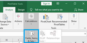
Selecting-fields-items-sets

Adding and Using an Excel Pivot Table Calculated Field

Step 4: Click on Calculated Field from the drop-down menu.

Clicking-calculated-field


The dialog box Insert Calculated Field appears. This is where you will name and create the field.

Step 5: Enter a name and Formula for the calculated field in the Name and Formula fields respectively.

Entering-name-and-formula


Note: Formulas can include standard operational signs and built-in program functions, however, they are incompatible with cell references and array formulas. Select the name of a field from the “Fields” box and click “Insert Field” to use it in your formula.

Step 6: Click on Add, the Calculated Field will appear as one of the fields in the PivotTable Fields list as soon as you add it, then Click on OK:

Clicking-add


How to Modify or Delete a Pivot Table Calculated Field?

After you’ve created a Pivot Table Calculated Field, you can modify or delete the formula by following these steps:

Step 1: Select any cell in the pivot table in your spreadsheet and Click on Analyze from the top ribbon.

Clicking-analyze


Step 2: Navigate to the Calculations tab.

Navigating-calculations-tab


Step 3: Select the option Fields, Items, & Sets.

clicking-fields-items-sets


Step 4: Click on Calculated Field from the drop-down menu.

Clicking-calculated-field


Step 5: Click the drop-down arrow in the Name field (small downward arrow at the end of the field).

clicking-dropdown-arrow


Step 6: Select the calculated field you want to delete or modify from the list.

Selecting-calculated-field-to-delete


Step 7: If you wish to modify the formula, change it, or click Delete if you want to remove it.

clicking-delete-option


How to Get a List of All the Calculated Field Formulas?

Excel makes it simple to generate a list of all the formulas used in the creation of Calculated Fields. The following are the procedures to easily obtain a list of All Calculated Fields formulas:

Step 1: Select any cell in the pivot table in your spreadsheet and Click on Analyze from the top ribbon.

Clicking-analyze


Step 2: Navigate to the Calculations tab.

Navigating-calculations-tab


Step 3: Select the option Fields, Items, & Sets.

clicking-fields-items-sets


Step 4: Click on Calculated Field from the drop-down menu.

Clicking-calculated-field


Step 5: Click on List Formulas.

clicking-list-formulas


Step 6: When you select List Formulas, Excel will automatically create a new worksheet with information about all the calculated fields and items you have used in the pivot table.

new-worksheet-created


Similar Reads

How to Create Excel Pivot Table Calculated Field with Examples
You can add calculated fields to a pivot table using your own unique algorithms that add up to other pivot fields. A calculated field has some restrictions, but it gives the pivot tables in your Excel worksheet a strong tool. What is a Pivot Table Calculated Field in Excel“Pivot Table calculated field” is an option to include more data or calculati
3 min read
How to Create Pivot Chart from Pivot Table in Excel using Java?
A Pivot Chart is used to analyze data of a table with very little effort (and no formulas) and it gives you the big picture of your raw data. It allows you to analyze data using various types of graphs and layouts. It is considered to be the best chart during a business presentation that involves huge data. To add a pivot chart to an Excel workshee
4 min read
How to Create Calculated Columns in Power Pivot in Excel
Power Pivot is an advanced data modeling tool that aims to perform advanced calculations on large datasets. Calculated columns are one of its features that makes it highly popular and help users derive new data by applying custom formulas to existing data columns. So, in this article, we will understand what are calculated columns, how to create th
5 min read
How to Remove Old Row and Column Items from the Pivot Table in Excel?
Pivot table is one of the most efficient tools in excel for data analysis. If you are using pivot tables frequently, then you will find even after deleting the old data from the data source, it remains in the filter drop-down of the pivot table. We will learn, how to remove the old row and column items from the pivot table in excel. Reason for not
4 min read
How to Troubleshoot and Fix Excel Pivot Table Errors?
Power Pivot is an Excel add-in, a data modeling technology that helps the user to create data models, establish relationships, and create calculations. However, it is possible to encounter a few errors during the process. here in this article, we will discuss some of the Excel Pivot Table Errors that may occur and how we can fix them. Usually, Exce
7 min read
Table and Chart Combinations in Excel Power Pivot
For data exploration, visualization, and reporting, Power Pivot offers a variety of Power PivotTable and Power PivotChart combinations. A Power PivotChart is a PivotChart that was made using the Power Pivot window and is based on the Data Model. Despite sharing certain functionality with Excel PivotChart, it offers additional features that give it
3 min read
Pivot Table Slicers in Excel
Slicers are the visual representation of filters. By using a slicer, we can filter our data in the pivot table by just clicking on the type of data we want. Slicers are found in the Analyze tab of the pivot table tools. We have an option called Insert Slicer and on clicking it, we have to select the column on the basis of which we need to filter ou
4 min read
How to Remove Pivot Table But Keep Data in Excel?
In this article, we will look into how to remove the Pivot Table but want to keep the data intact in Excel. To do so follow the below steps: Step 1: Select the Pivot table. To select the table, go to Analyze tabSelect the menu and choose the Entire Pivot Table. Step 2: Now copy the entire Pivot table data by Ctrl+C. Step 3: Select a cell in the wor
1 min read
How to Delete a Pivot Table in Excel?
A pivot table is a tool in Excel that allows you to quickly summarize data in the spreadsheet. When it comes to deleting a Pivot Table, there are a few different ways you can do this. The method you choose will depend on how you want to delete the Pivot Table. 1.Delete the Pivot Table and the Resulting Data. Steps to delete the Pivot table and the
3 min read
Refresh Pivot Table Data in Excel
In the Pivot data table, data can be grouped based on Dates, Numbers, and Text values. In the case of dates, we can group dates by months or year, months by years, etc. At any time, data for the PivotTables in your workbook can be refreshed using the Refresh button. You can also refresh data from a source table in the same or a different workbook.
2 min read
Article Tags :