What I wish someone had told me when I started learning about File System Forensics

 Many of the concepts and the definitions mentioned in this blog post are referenced from [Brian (2005)] File System Forensic Analysis and libfsntfs documentation by Joachim Metz. 

If you’re new to Digital Forensics a first question you might be asking is: why do I need to learn how file systems work as a digital forensics analyst? And how much do I need to know about it?

Why do we need File System Forensics?

Let’s answer that question starting with a very simple definition of digital forensics. Digital forensics is typically used to determine what happened after the fact. Throughout a digital forensics investigation this question will very likely be broken down to multiple smaller questions.

For example an analyst might start their investigation with an alert from a network based intrusion detection system, warning them that a certain host in their network is communicating with a malicious domain attributed to an active threat group, known to be targeting their industry. The analyst may start to craft one question after the other, trying to understand what happened and to progress in their investigation, such as: 

• Which process on the identified host is communicating to the malicious domain? 

• Is the executable file that launched this process still on disk, in memory, or was it deleted? 

• Did the executable open network connections to other hosts on the network?

• What are other related system events around the time of execution?

While answering these questions, different forms of evidence, such as a non-volatile storage device, a memory capture, system logs, etc. are the subject of the investigation.

Non-volatile storage devices

There are different forms of non-volatile storage devices. The most dominant forms of physical storage devices in today’s computers are the (magnetic) hard disk drives (HDDs) or solid-state drives (SSDs). Nowadays these storage devices are often virtualized and utilized as virtual disks in virtualized computing environments, such as Cloud computing. In this article we will use the term storage device and hard disk interchangeably to equally refer to HDD, SSD and virtual storage with disregard to the differences in the underlying technologies utilized by each of them. Non-volatile storage devices typically contain one or more file systems. 

Preserving non-volatile storage devices

To preserve a storage device as evidence we first need to reliably acquire the data from the device. There are several ways to do so, since the data can be accessed on different layers of the technology stack used in modern computers and shown in Fig.1. The evidence we are searching for might be within one of these layers. For example a permanently deleted file can’t be found if we try to read it via the operating system installed on the hard drive, however it might still be present in the unallocated areas of the hard disk.

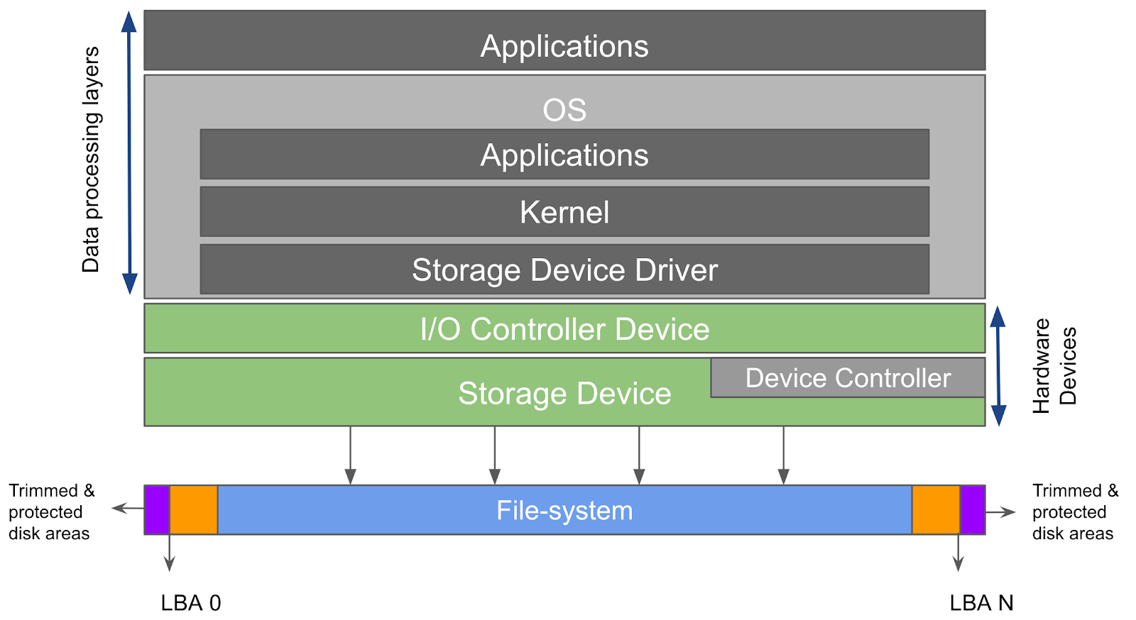
Fig. 1. Data processing layers in OS and different storage device segments

So ideally we need to acquire the data on the lowest possible layer, i.e. closest to the silicon as possible. It is worth mentioning here that, during the acquisition of storage media devices, disk access can happen on multiple layers as well. For example accessing the disk via the computer firmware (BIOS) means that we will access and acquire the data blocks exposed by the Logical Block Addressing (LBA) as shown in Fig. 1, LBA provides a linear address space of the storage device to the host while abstracting the details of physical sector positions, thus we are acquiring on the logical block level rather than physical block level.

The full range of LBAs is what is often acquired when we hear “we made a bit-by-bit copy of the entire hard disk”, however there are other areas on the hard disk outside the LBA space, often referred to as service area or system area, the service area stores several modules necessary for managing the hard disk, such as managing corrupt storage blocks, self-test modules, etc.

The service area of a disk is accessible via sending vendor specific commands directly to the hard drive’s IO ports. These commands are specific to every vendor and are not necessarily publicly disclosed, although hard drive vendors release tools for manipulating hard drive’s management functionalities. The service area can theoretically be used, via vendor specific commands, to read and write data that are otherwise inaccessible. This should not be confused with protected disk areas such as Device Configuration Overlay (DCO) or Host Protected Area (HPA) in ATA disks as shown in Fig. 1, which can be accessed via standard ATA commands and used to hide data.

Long story short, typical forensics tools used for image acquisition commonly utilize one of two different methods, first is to access the disk as a block device via the computer firmware and acquire the blocks of data on a hard disk (the LBA space), second is to acquire protected disk areas, such as HPA and DCO in ATA disks or other areas in disks that use different interfaces, via direct disk access. SSD disks need to be put into a special mode (factory mode) in order to acquire the protected and trimmed disk areas.

There can be multiple interpretations of what people mean by “we acquired a raw disk image” or “we made a forensics copy of the disk”, thus you have to be careful with understanding how acquisition happened. For example, in cloud storage all data is logical, however there are still different layers, e.g base and differential images, to consider while acquiring disks. For more information regarding the procedures of disk acquisition in the Cloud, also see  blog post about Libcloudforensics.

In this section, we discussed the different types of storage devices and some caveats about preserving non-volatile storage devices. In the next section of this blog post we will start digging into the file system structures, with focus on different data types, data storage procedures and forensics artifacts of a file system.

File Systems

A file system can be seen as a hierarchical set of data structures, consisting of data and metadata, and procedures to update these data structures. The raw data that forms the file system structures typically reside on a storage device. In a digital forensics investigation we may decide to examine and interpret file system structures stored in a volume. Via interpreting these file system structures, according to the predefined rules in the file system specification, the analyst can list files and directories on the system, recover deleted content, find timestamps for file system events, such as file/folder creation, deletion, access or modification operations, etc.

It is also worth mentioning here that, similarly, forensics tools access data on different layers of the technology stack. For example, some tools directly access the raw bytes of data on a storage device or a disk image, such as Linux Strings, while other tools interpret the file system structures, such as Plaso. It is important to understand how different tools work and how they access data, in order to determine the most suitable tool to use in your specific case.

File System Data Organization

To get your head around the main concepts of file system data organization, let’s start with the main data categories of a file system (Brian 2005). These data categories are not tied to a specific file system and can be used as a basic reference model to compare different file systems. This model is adopted by some of the computer forensics tools to analyze file systems, such as The Sleuth Kit (TSK). 

Data Categories

1. File system data category (aka file system metadata): think of the site map of a very large website, similarly the data in this category, which are typically independent values, represents the layout information of the file system on disk, such as; the location of the boot code, the location of the allocation-bitmap (an array of ones and zeros that tells which data unit (ex: block or cluster), of the file system is free and which data unit is allocated to a file or a folder). If the file system structures are corrupt and you are left in a situation, where you have to start recovering data by hand, the information in the file system metadata will be very useful. 

2. Content data category: this category refers to the storage locations that are allocated to files, directories, symbolic links and their content data. The data in this category are typically organized into equal sized groups, which have different names in different file systems such as cluster or block, in general this can be referred to as a data unit. A data unit is either allocated or unallocated. There is typically some type of data structure that keeps track of the allocation status of each data unit (e.g. bitmaps). 

3. Metadata data category: metadata is data that describes data (content), such as the last accessed time and the addresses of the data units allocated to a file. This category does not contain the content of the file itself, and it may or may not not contain the name of the file. Most forensics tools typically merge the metadata category with the filename data category. However they might come from different sources, depending on the file system analyzed.

4. Filename data category: includes the names of files, and it allows the user to refer to a file by its name instead of its metadata address. At its core, this category of data includes only a file's name and its metadata address. Some file systems may also include file type information or temporal information, but that is not standard. In most file systems, these data are located in the contents of a directory and are a list of file names with the corresponding metadata addresses.

5. Application data category: data in this category are not essential to the file system, the only reason they exist as special file system data instead of inside a normal file, is because this is more efficient. One of the most common file system structures that falls in this category is the file system Journaling; a crash can occur while a system is writing data to the disk, this can leave the system in a bad state next time it starts, for example: new metadata entry is created which points to a content that doesn’t yet exist on disk. Journaling solves this problem, before any metadata changes are made to the file system, an entry is made in the journal that describes the changes that will occur. After the changes are made, another entry is made in the journal to show that the changes occurred. If the system crashes, a scanning program reads the journal and locates the entries that were not completed.

NTFS File System

Let’s explore the New Technologies File system (NTFS) with the previously mentioned data categories of a file system in mind. NTFS is the most common Windows file system and most other file systems will follow similar principles. Learning about all the details of NTFS is beyond the scope of this article, however we will cover the basic principles. If you want to learn more about the specifics of NTFS file system, refer to the libfsntfs or equivalent documentation.

As mentioned before; a file system has a data-unit, NTFS refers to its file system blocks as clusters (or cluster blocks). Note that these are not the same as the physical clusters of a hard disk. Typically the cluster block is 4096 bytes of size (historically 8 sectors of 512 bytes). In NTFS everything is a file, including the data of the file system data category. Therefore the entire file system is considered a data area. 

“The Master File Table (MFT) is the heart of NTFS because it contains the information about all files and directories. The MFT is a file in itself named $MFT. Every file and directory has at least one entry in the table, and the entries by themselves are very simple. They are typically 1024 bytes in size. The first 42 bytes of an MFT entry have a defined purpose, while the remaining bytes store attributes, which are small data structures that have a very specific purpose. For example, one attribute is used to store the file's name, and another is used to store the file's content. Fig. 2. shows the basic layout of an MFT entry” (Brian 2005).

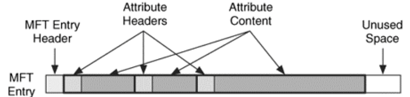
Fig. 2. MFT entry layout
[Brian (2005)] File System Forensic Analysis, chapter 11

Each MFT entry has one or more attributes, the attribute properties, i.e. type, size and name are defined in the header field. The content of an attribute has no defined format or size, if the content fits within the MFT entry, it will be stored there as a resident attribute. If the content doesn’t fit into the MFT entry it will be stored into an external cluster block in the file system and referenced in the attribute content, in that case it is called a non-resident attribute. The attribute header will have a flag specifying if the attribute is resident or non-resident. There is a long list of attribute types used in NTFS, a full list can be found in libfsntfs documentation.

Back to the file system data category or the file system metadata files, the first 16 MFT entries are reserved for the file system metadata files. Each of the file system metadata files, referenced within the first 16 entries of the MFT, is located in the root directory of the file system. Table 1 shows a list of the first 16 entries of the MFT table (file system metadata files) and their description.

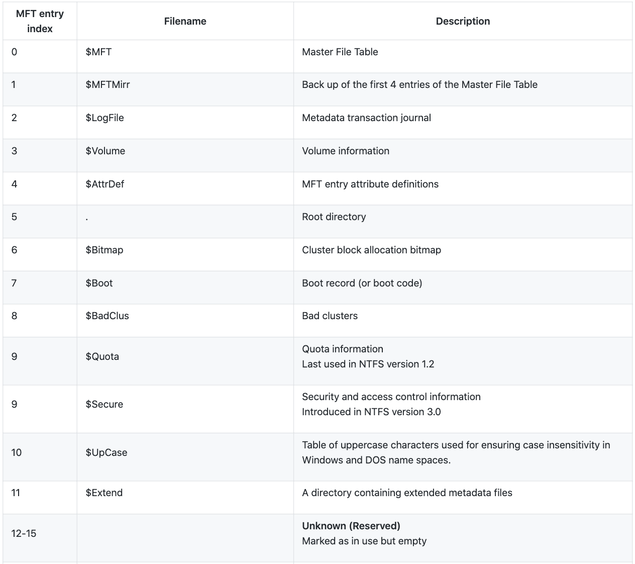
Table 1. The first 16 MFT entries and their description as per libfsntfs documentation.

The content data category is stored, either as resident $DATA attributes in $MFT entries or as allocated clusters on the storage device, in the case of a non-resident $DATA attribute in $MFT, the $MFT attribute will only store the offset of the cluster storing the data and the data length, while the data itself will be stored in the allocated disk clusters. It is worth mentioning that the data can be stored in fragments; where partial fragments of the file are stored at different clusters, data runs will hold the range of clusters storing the data. Data runs are stored as attributes in $MFT entries. Data fragmentation, and how it is realized in a file system, can be a decisive factor when you choose your data carving tool/algorithm.

The content metadata category of the file system is stored as attributes in the $MFT entries representing the data (files or directories). Most important is: 

• $STANDARD_INFORMATION attribute which holds 4 timestamps recording; the content modification time (M), access time (A), metadata (MFT entry) modification (or change) time (C), and creation (or birth) time of a file (B), these timestamps are typically referred to as MACB.

• $FILE_NAME attribute which holds 4 other timestamps (MACB). The $FILE_NAME attribute also holds the filename data category; including the parent MFT entry and the filename. The attribute is stored as a resident MFT attribute. It is important to understand the effect of different file system events on those timestamps, note that these changes differ with different NTFS implementations. For example mkntfs might behave differently than Windows XP or later versions of  Windows. Examples of some of the timestamp behavior observed for Windows 10 NTFS implementation, can be found on the Cyber Forensicator poster.

The $FILE_NAME attribute in NTFS can also be found in directories ($I30 index). Directories in NTFS are indexes of filenames and are realized via B-Tree structures, to realize the hierarchical architecture of directories and files. 

NTFS file system is a (metadata) journaling file system, the file system metadata journal falls under the application data category and is realized via the metadata file named $LogFile. This file contains the metadata transaction journal. Parsing a file system metadata journal can provide information about recent file system changes. This can be a valuable source of data in some investigations; for example, you might be able to prove the existence of a file, before being deleted with no metadata left behind in $MFT.

Conclusion

In case of a forensics analysis of a file system, understanding how the file system was acquired, the data structures of that file system and how different tools access and parse these structures, is in many cases the key to solve the outstanding forensics questions.

For example in some cases the attackers may manipulate timestamps to make the creation of a malicious file less obvious in a timeline. This can be achieved in several ways and via multiple tools, such as Timestomp, SetMACE, and nTimestomp. These tools mostly rely on Windows API functions (NtSetInformationFile, SetFileTime) to manipulate the timestamps of a file, although they utilize different techniques to make detection harder. These API functions allow a caller to set any of the $STANDARD_INFORMATION MACB values to a 64-bit value of their choice, however they can’t be used to alter the $FILE_NAME MACB timestamps.

With the understanding of NTFS previously described we know that the timestamps in the $FILE_NAME mirror those of the $STANDARD_INFORMATION timestamps. The $FILE_NAME timestamps are typically set when the file is created and cannot be altered directly using the previously mentioned API functions. Detecting timestamps manipulation, in some cases, can be done via identifying inconsistencies between the values of the $FILE_NAME timestamps and the values of the $STANDARD_INFORMATION timestamps.

This is one of the many examples on how an analyst's knowledge about the specifics of a file system can help them solve a forensics riddle!