The number of trees growing in a forest at any point in time shapes the look and character of a woodland and determines the benefits woodland owners may reap from it. A thorough look at competition and stand density can help landowners get the most out of their woods.
Family forest landowners have many aims and expectations for their property. The objectives of small woodland owners are generally quite different from those of their neighbors who manage industry or government land.
Many people want an attractive, peaceful place to live or play in privacy, as well as a place that is diverse and welcoming to wildlife and human visitors. They view it as a personal and economic investment, and a legacy that they hope to leave for heirs. Although timber production is not a primary motivation for most family landowners, it is important for some, and periodic income from property is often seen as a way to help pay the bills or make desired improvements.
The main strategy for meeting many family landowners’ objectives is to grow older forests. Both stand age and disturbances, such as thinning to reduce density and competition, can enhance development of many desired stand characteristics.
Relative density as an indicator of competition
RD is our best measure of crowding and competition in a stand of trees. It relates well to other common indicators such as tree growth rates, crown depth, and self-thinning. Those other indicators are useful in the present but less helpful predicting the future. Because we can quantify and predict future RDs, we can use RD to anticipate future competition and determine when to take future management actions.
How this applies to your woods
Competition among trees has a powerful effect on the growth, health, resiliency, and character of a woodland. It affects trees individually, but also as a group or “stand” of which each is a part. Therefore, it is important for woodland owners to be aware of the degree of competition influencing trees within a stand.
Competition affects an individual tree’s growth rate, and therefore diameter, taper, maximum branch size, and the width of annual growth rings. Competition also affects a tree’s vigor and its ability to tolerate or resist insects, diseases, and storms.
Competition shapes the development of a stand and of stand-level characteristics, including the size of trees, the size of the green crown (crown length or depth), the forest structure (for example, size variability), stand volume, and both the type and amount of other plants growing on the forest floor and beneath the main forest canopy (the understory).
Stand density management is not just academic. These different tree and stand characteristics that result from changes in stand density are important in determining how well a stand meets a landowner’s specific management objective, such as habitat diversity or optimal timber quality or yield. It is up to landowners to choose the right degree of competition during the life of the stand to get the results they want.
Stages of competition
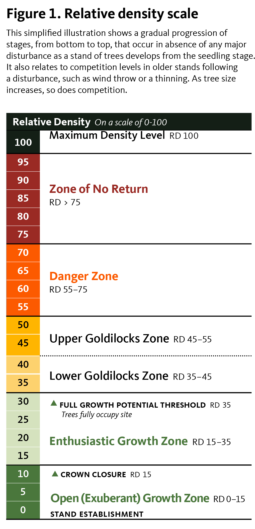
As trees grow from uncrowded seedlings toward a group of larger trees approaching maximum density level (RD 100) without a major disturbance, the stand passes through certain stages along the way. These stages correspond with predictable levels of competition at anticipated RDs that have been identified through years of forestry research. It is important to be familiar with these stages, the amount of competition occurring, and its impact on tree and stand characteristics. See Figure 1.
Let’s look at the key stages of competition, including approximate RDs at which they occur. These descriptions apply best to development in undisturbed, even-aged stands of a single species, but can also reflect competition levels following a disturbance or give insight into competition pressure when managing mixed species. Disturbances that kill trees may be natural occurences (such as wind throw) or intentional human activities (such as harvesting trees in a thinning or when creating an opening).
Either type of disturbance temporarily frees up growing space, lowers stand RD, and delays progression to the next stage. Large disturbances may change the RD enough to shift a stand back into an earlier and less intense stage of competition.
By lowering the RD and the level of competition, the disturbance changes not just the timeline but also the look and character of the stand and the trees within it.
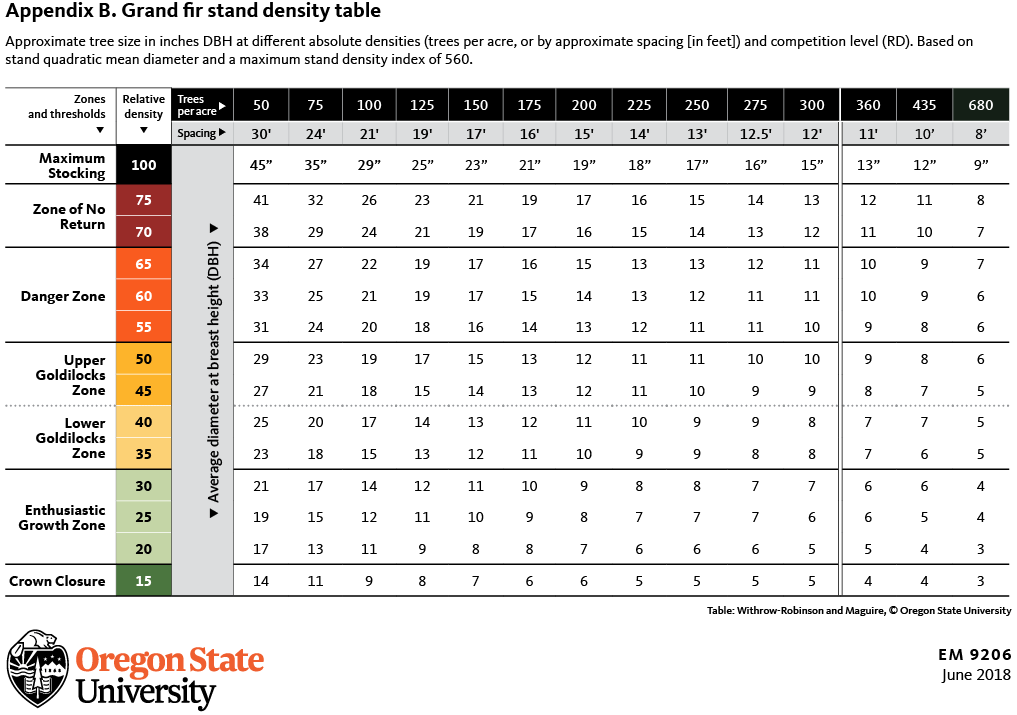
Stand density tables
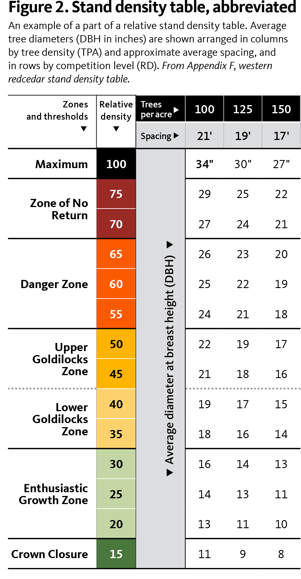
Woodland owners can learn to visualize and apply these competitive forces and biological limitations with the use of relative stand density tables. These tables provide information about three interdependent factors: stand density (trees per acre, or TPA), tree size (average diameter at breast height, or DBH) and level of competition (RD). We use these tables to estimate current levels or predict future levels of one of these factors, based on the other two.
Stand density tables come in a variety of configurations. We have arranged our tables in a new way, according to stand density and competition level to reveal tree size. In Figure 2, columns are arranged by increasing density (TPA)—from a few trees to many trees—from left to right. The rows are arranged by increasing competition and RD (see the second column), from less competition to more competition, from bottom to top, as illustrated in Figure 1 (page 3).
The intersection of a column and a row reveals the average size of tree (in inches DBH) at that number of trees per acre and level of completion (RD).
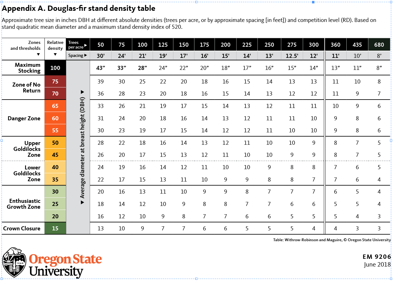
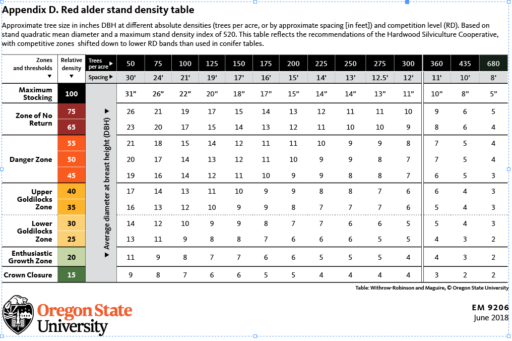
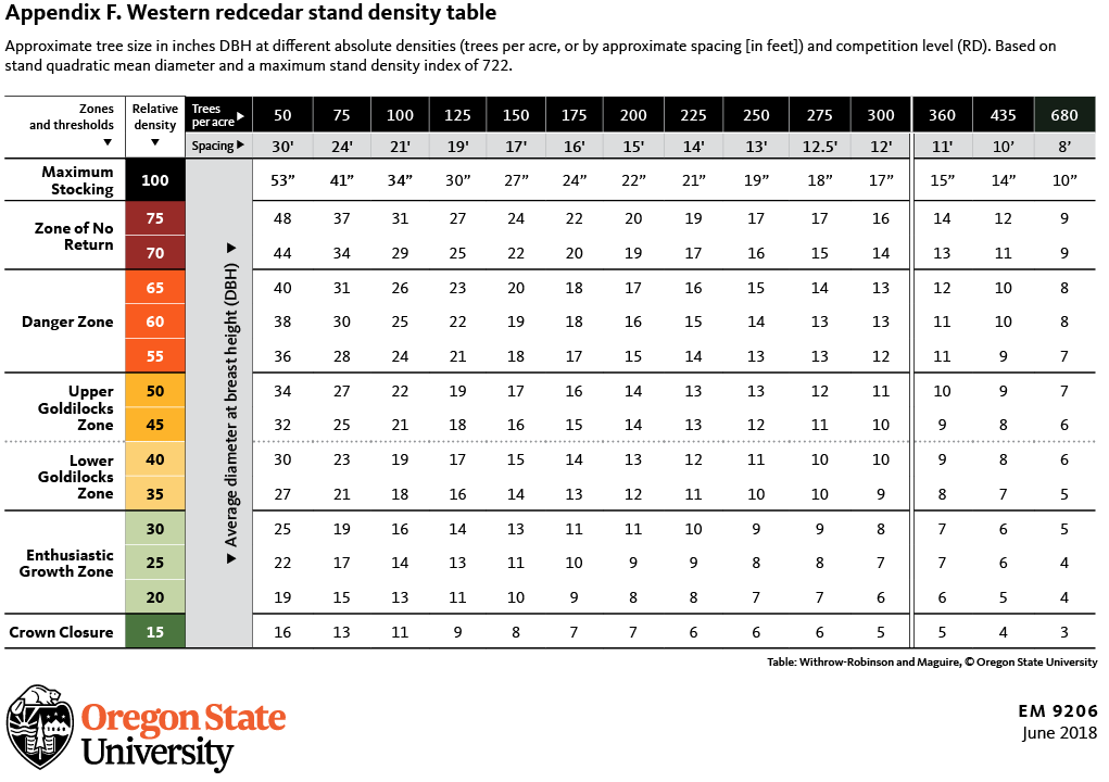
This configuration of a relative stand density table allows a woodland owner to visualize and anticipate how a stand progresses through competitive stages as it develops over time, and helps predict future levels of competition that will arise in the stand as the trees grow. See the Appendices (starting at page 11) for relative stand density tables for several different species, each with density and DBH values appropriate for that species.
Understanding the stand density table
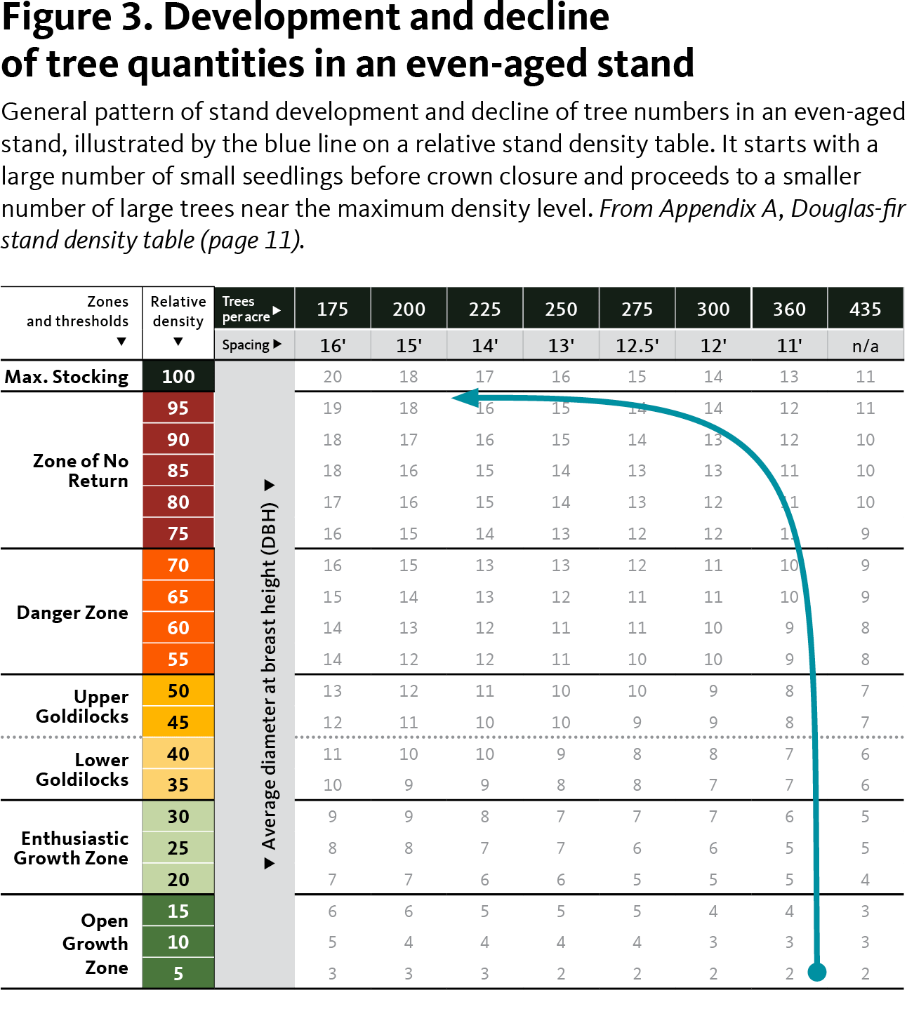
Let’s look at how this table illustrates competition and stand development. Imagine a new (even-aged) stand starting off with a given number of seedling trees, about 360 trees per acre, as represented by a blue dot in Figure 3. The trees begin growing without much competition, and so survival is good and few trees die initially. As the trees grow, they gradually and increasingly crowd and compete with each other. Tree growth gradually slows. In the absence of a major disturbance, the number of trees holds steady through the green Open and Enthusiastic Growth zones and the yellow Goldilocks zones. The straight vertical portion of the dotted line in Figure 3 illustrates this period of growth. When the trees eventually become so crowded that some begin to die (or self-thin), the number of trees declines in the orange Danger Zone. This decline is illustrated by the curved section of the growth line that turns to the left in Figure 3.
As stressed trees die, the growing space vacated by the dying trees can be used by the surviving trees, allowing them to grow larger. Thus, the line representing the number and size of trees in the stand continues to drift left as the number of trees decreases and upward as the surviving trees grow gradually larger. This continues through the red Danger Zone before flattening out in the brown Zone of No Return, just below the maximum density level.
Using a stand density table to guide your actions
A stand density table can help you make important decisions about your woodland. A density table can tell you when and how much to thin (at what stand diameter and to what new density). This lets you keep a stand growing within a desired range of competition, which helps to develop the conditions you want. You can also use the table to decide if a young stand thinning (also called pre-commercial thinning) is needed to allow room for trees to reach a target diameter and prevent overcrowding and stress.
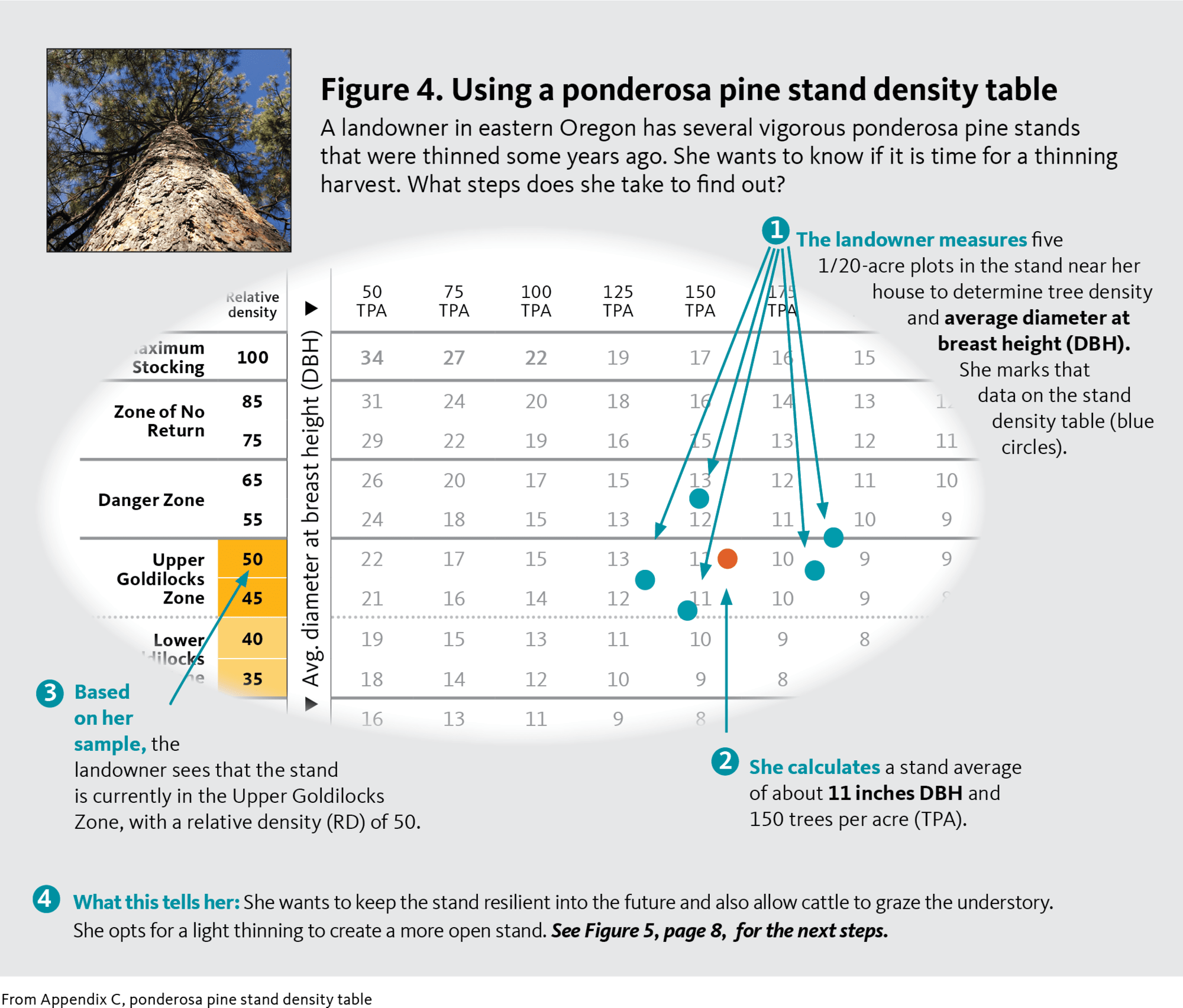
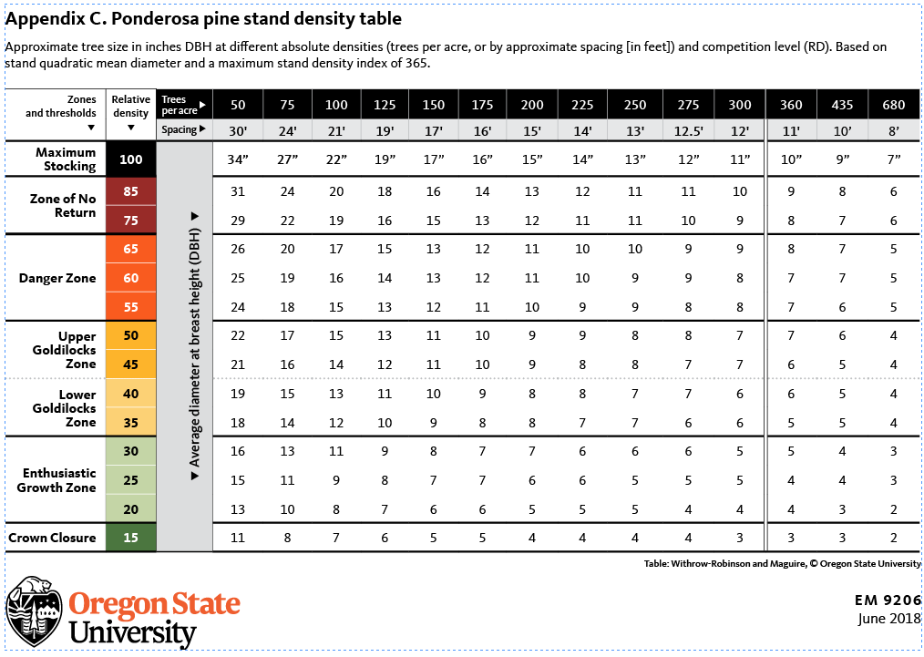
Let’s take an example of a landowner in eastern Oregon who has several vigorous ponderosa pine stands that were thinned some years ago. She is concerned about keeping the trees vigorous and resilient to drought and insect threats, and she also seeks to produce some forage for grazing. She wants to know if it is time for a thinning harvest.
To get an idea, she goes out to the small stand nearest her house to get current information. Referring to Measuring Your Trees (EM 9058), she measures a sample of five ¹/₂₀-acre plots to determine tree density and average DBH for each. She then marks the data on a copy of the stand density table (blue circles, Figure 4). The plot average for tree density and DBH varies among the samples, but she calculates a stand average of about 11 inches DBH and 150 TPA (red circle A, Figure 4). Based on her sample, she sees that the stand currently has an RD around 45–50, in the Upper Goldilocks Zone.
She now needs to figure out what this information means to her. The stand’s RD is below the point generally seen as the upper limit a stand should be allowed to reach before thinning (RD 55), so she can consider allowing it to grow longer. However, she knows that too much competition can predispose trees to damage from insects and other problems, especially in times of drought. She hopes to avoid that risk by keeping the stand vigorous and resilient to stress, and is willing to sacrifice some potential stand growth to gain that. She would also like to allow some light cattle grazing of the understory, which would benefit from a more open stand. She decides that keeping the stand’s densities between RD 35 and RD 50 would best meet her objectives. This means that if her sample is representative of the rest of her stands, it is time to plan a thinning.
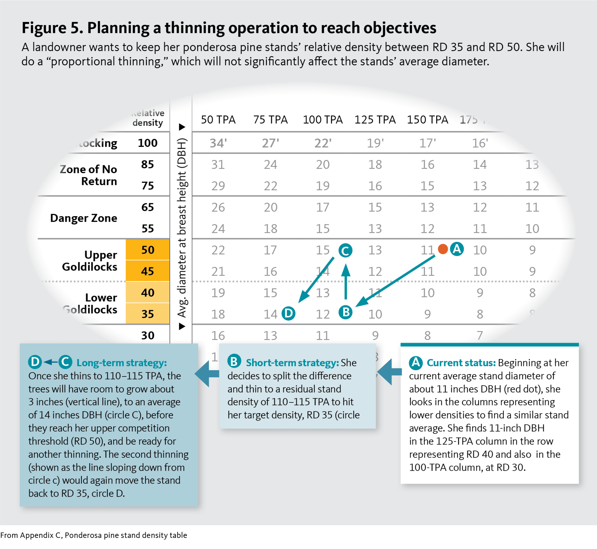
Now she can use the stand density table to help (Figure 5). She anticipates a “proportional thinning.” This means she will take trees from across the size range, meaning the thinning will not significantly affect the stands’ average diameter. Beginning at the point representing her current stand average in the discussion above (Figure 5, circle A), she looks to the columns representing lower densities to the left to find a similar average tree size (11-inch DBH). She finds this under the 125-TPA column, in the row representing RD 40 (in the yellow Lower Goldilocks Zone). She also finds 11-inch DBH in the 100-TPA column, in the row representing RD 30 (in the green Enthusiastic Growth Zone). She decides to split the difference and thin to a residual stand density of about 110–115 TPA for a RD of about 35, at the bottom of the Lower Goldilocks Zone (Figure 5, circle B).
The table also lets her look ahead. She sees that if she thins to the target 110–115 TPA, the trees in the stands will then have room to grow about 3 inches (Figure 5, vertical line [page 8]) to an average of around 14 inches DBH (Figure 5, circle C [page 8]), before they reach her upper threshold (RD 50) at the top of her chosen target range. They would then be ready for a second thinning harvest, which would again move the stand back to the lower target density (RD 35) at Figure 5, circle D (page 8).
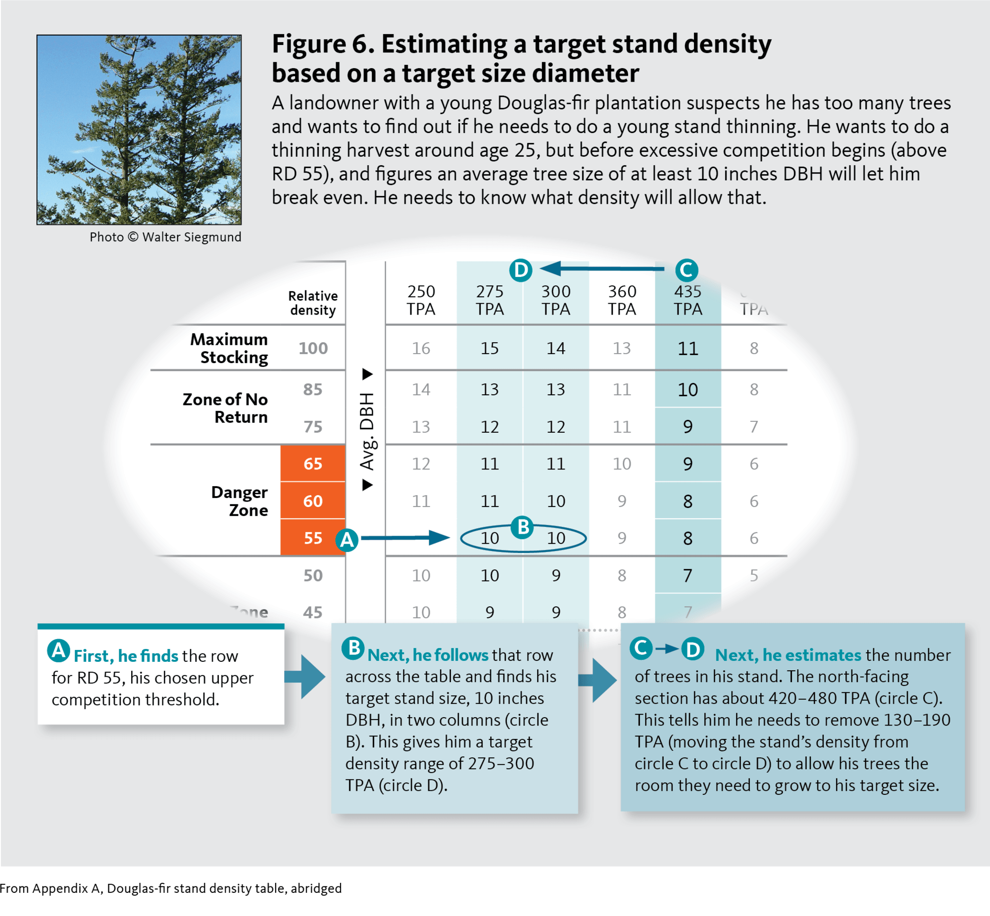
For our next example, a landowner with a 12-year-old Douglas-fir plantation in western Oregon had good survival at planting and is now concerned that he has too many trees and that they will become too crowded before they are large enough to be ready for a first thinning harvest at age 25 or so. He wants to cover the costs of the operation by selling the logs he thins. Based on the markets in his area, he figures he needs a stand with an average tree size of at least 10 inches DBH at the time of the first thinning harvest to “break even.” He knows he wants the stand to reach that target size before excessive competition begins (avoiding the danger zone above RD 55) and needs to estimate the stand density (TPA) that will allow that. He can use the Douglas-fir stand density table to figure this out.
He starts by finding the row for RD 55, his chosen upper competition threshold (Figure 6, circle A) and then follows that row across the columns to the right until reaching a column with his target stand size, 10 inches DBH. He finds that in two columns (Figure 6, circle B). This gives him a target density range of 275 TPA and 300 TPA (Figure 6, circle C).
Next, he needs to know the density of trees (TPA) he has in his young stand. He estimates that with plots as described in Measuring Your Trees (EM 9058) and compares it to his target density to decide if he needs to do a young stand thinning (also known as PCT). He finds a lot of variation in his measurements, especially on the two different sides of a draw that runs through the stand. On the south-facing side, his plots range from 240 TPA to 340 TPA, but were generally around 300 TPA. Survival is higher on the north-facing side of the draw. There his plots range from around 420 TPA to 480 TPA, which is sometimes more trees than he planted due to natural seeding from the adjacent mature stand.
So what does this mean? Since his young stand on the south-facing slope generally has a similar number of trees per acre as his target density, he is on track to reach the desired average tree diameter. But the north-facing part of the stand (Figure 6, circle D [page 9]) generally has significantly more trees per acre than his target density, so he is NOT on track. He needs to consider a young stand thinning (YST) to correct that.
With this information in hand, he decides to leave the south-facing section alone and pursue a young stand thinning in the north-facing section. He will need to remove 130–190 TPA in various parts of the planting to bring the stand density down to 290 TPA, the midpoint of his target range (Figure 6, circle D to circle C ([page 9]). This will allow his trees to reach the desired average tree diameter before experiencing significant harmful competition.
Conclusion
Understanding the effects of competition on how trees grow and how forest stands develop is critical to shaping the conditions you want on your property. Managing for or restoring desired conditions is easier if you understand that competition develops in a predictable manner and that a developing forest moves predictably through zones of increasing competition.
Relative stand density (RD) is an important tool for estimating the competition within stands and understanding where a stand falls in the progression of competitive stages. Stand density tables use relative stand density to help landowners understand and manage the competition in their forest stands and shape the future of their woodland property. It is up to the landowner to control competition during the life of the stand to achieve desired goals.
Resources
OSU Extension publications
Find these and other Oregon State University Extension Service publications online at catalog.extension.oregonstate.edu/
- Tools for Measuring Your Forest (EC 1129), catalog.extension.oregonstate.edu/ec1129
- Measuring Your Trees (EM 9058), catalog.extension.oregonstate.edu/em9058
- Basic Forest Inventory Techniques for Family Forest Owners (PNW 630), catalog.extension.oregonstate.edu/pnw630
- Thinning: An Important Timber Management Tool (PNW 184), catalog.extension.oregonstate.edu/pnw184
Other resources
Management by Objective http://blogs.oregonstate.edu/treetopics/2015/02/10/management-objective/
Brad Withrow-Robinson, Forestry & Natural Resources Extension; and Doug Maguire, Giustina professor of forest management and director, Center for Intensive Planted-forest Silviculture, Oregon State University
Defining some terms
- Competition occurs among trees because the amount of resources needed to support plant growth (light, moisture, or nutrients) is limited. Each tree needs more of those resources as it grows larger. This increasing demand means that as the trees grow, resources will eventually run short. Competition increases among trees as they struggle to get what they need from the site.
- Stand density is a measure of the number of trees and how fully the trees occupy a site. We can think about density in either absolute or relative terms.
- Absolute stand density is the number of trees per unit area (typically the number of trees per acre, or TPA).
- Relative stand density (RD) indicates how fully the trees occupy a site. Relative stand density is a measure of the number and average size of trees growing in a stand compared to the maximum possible number of trees of the same average size that the site could support (a biological limitation). It tells us how crowded the trees are and measures the intensity of competition. RD is expressed on a scale of 0–100 percent, where 0 is an unoccupied site and 100 represents the potential maximum density for that species. Maximum density levels vary dramatically between species, but only slightly by location and site for a given species. Both absolute and relative stand density can change dramatically over time. Absolute density changes when the number of trees changes, for example, as new trees seed in or as established trees die. Relative density increases or decreases along with corresponding changes in absolute density, and also when a fixed number of live trees grow bigger.
Stages of increasing stand competition
Open (Exuberant) Growth Zone RD 0–15
Although seedlings or young trees may compete with leafy (herbaceous) or woody (shrub and tree) vegetation during the establishment stage, they are not yet competing with each other and should have lots of room to grow. Crown closure occurs for a young stand around RD 15.
Enthusiastic Growth Zone RD 15-35
Usually seen in young stands following crown closure when trees still have plenty of room and resources (water, nutrients and light) but are beginning to compete with each other and with any other woody plants in the stand. Lower branches begin to decline and die as they become increasingly shaded (a process called “self-pruning”). The bottom of the live crown begins to move up the stem in what is called “crown lift” or “crown recession.” The understory becomes sparse. Understory plants shift to shade-tolerant species. Full growth potential threshold is reached as trees fully capture the site (around RD 35).
The Goldilocks Zone RD 35–55
Traditionally thought of as the “optimum growth zone” by foresters, we call this the Goldilocks Zone because it is seen as “just right”: not too open, not too crowded. It is a zone of robust growth and the zone in which many managers often try to maintain stands for decades with repeated thinning. Individual trees are generally robust, so stands are vigorous and resilient to stress and pests. Stands in this zone are conducive to thinning. Trees typically respond well in growth and remain stable afterwards. Thinning intensity is geared for a return to the pre-thinning RD within 10 or so years. Managers can achieve many different objectives—ecological, economic and social—from stands in this zone.
Lower Goldilocks Zone RD 35–45
In young stands, trees fully control the site and most of its resources. Competition between trees intensifies. The trees begin to separate into different into “crown classes” (See Thinning: An Important Timber Management Tool, PNW 184), but crowns are generally deep enough (40 to 60 percent crown ratio) to support robust tree growth. With repeated thinning, older stands can be maintained to meet non-timber objectives without too adversely reducing stand growth. Stands are spaced widely (open) enough to allow light to penetrate the canopy. This helps maintain deep crowns and supports understory growth, which is important to providing habitat for many species. To meet certain habitat objectives, it may be desirable to reduce competition below the Goldilocks Zone for some period, perhaps to as low as RD 25.
Upper Goldilocks Zone RD 45–55
Competition is more intense in the upper parts of the Goldilocks Zone. Here we see continued crown lift and further differentiation of individual trees into crown classes in young stands. Average crown depth decreases (30 to 50 percent). This keeps maximum branch size small and stem-form more cylindrical (meaning, less taper). Dense shade limits the type and growth of understory vegetation. Individual tree growth is strong, although decreasing, especially among lower crown classes, but volume growth of the stand is high. The Upper Goldilocks Zone is generally seen as “just right” when it comes to optimizing timber quality and quantity.
Danger Zone RD 55–75
Trees compete intensely for resources. We see rapid and continued crown lift and wider differentiation into crown classes. This means the average crown lengths become dangerously small—especially the smallest overtopped trees. Some trees fail to get the resources needed. Weaker trees die, freeing up resources that allow surviving trees to grow. When trees die because of competition, we say the stand is “self-thinning.” Foresters call this “competition mortality,” or “suppression mortality” and call the area above RD 55 the “Zone of Imminent Competition Mortality.”
Trees in the Danger Zone tend to be skinny for their height, with small, narrow crowns. The proportion of the tree length with live branches continues to decline, and trees become steadily more stressed. They tend to have little taper, small branches and tight growth rings. Stand-level volume growth can remain high. The understory tends to be sparse. This is an acceptable condition near the end of a rotation prior to final harvest. But it is not a good condition if the landowner wants to keep the stand longer, to harvest some trees in late thinnings, or to develop different stand conditions.
We call this the Danger Zone to highlight the rapid loss of options, rather than the natural loss of trees. The longer a stand remains in this zone, the more poorly it will respond to thinning with renewed growth, and the more likely the stand will be unstable and easily damaged by wind or wet snow. The window of opportunity to thin the stand narrows, depending on how much the crowns have differentiated. If the stand stays in this zone for long, the landowner has, in many cases, missed the opportunity to manage for different stand conditions.
Zone of No Return RD 75
This zone is characterized by many small, skinny, and stressed trees with small crowns and active self-thinning. Even the dominant trees may have small, weak crowns. For many stands arriving at this point, it is too late to thin. Stability of residual trees is frequently poor if the stand is opened up. Once a stand reaches this stage, the best option is often to leave it alone until the time arrives for a regeneration harvest (a clearcut or shelterwood cut) to start a new stand.
Taking stock of stand diameter
An individual tree’s diameter is measured at breast height (DBH), or 4.5 feet above the ground on the uphill side of the tree. But there are several ways to calculate the average diameter of the trees in a stand, or stand diameter.
Foresters generally use the Quadratic Mean Diameter (QMD) to calculate stand diameter. The QMD is the diameter of the tree of average basal area (BA) for a stand. Growth models, density management diagrams, and stand density tables are developed based on the QMD.
The QMD is used for calculating stand density because it accounts for variability in a stand better than the average DBH does, and it is readily converted into stand basal area. This is important because there is sometimes a great deal of variation in the size of individual trees within a stand. A simple average tends to underestimate the effect of the larger trees in those situations.
Most people would rather calculate the average stand DBH to make their decisions. Although this creates some room for error, it is probably a reasonable practice for family landowners in many circumstances.
For instance, the difference between the average DBH and QMD tends to be quite small in uniform stands, with small differences in tree sizes. For many young, planted forests growing on private lands, particularly in western Oregon, the difference between the two measures would probably be unimportant for most management decisions.
The difference between the two measures becomes greater as the stands become less uniform. A simple stand average DBH would become less accurate (underestimating the larger trees) in older or uneven aged stands, as is more typical of managed stands in central and eastern Oregon. In these situations, it may be prudent to calculate the stand QMD, or perhaps hire a consulting forester to cruise your stand.
See Measuring Your Trees (EM 9058) for information on forest inventory measurements and calculations. This publication covers plot layout, measurements and calculation of QMD.
© 2018 Oregon State University.
Extension work is a cooperative program of Oregon State University, the U.S. Department of Agriculture, and Oregon counties. Oregon State University Extension Service offers educational programs, activities, and materials without discrimination on the basis of race, color, national origin, religion, sex, gender identity (including gender expression), sexual orientation, disability, age, marital status, familial/parental status, income derived from a public assistance program, political beliefs, genetic information, veteran’s status, reprisal or retaliation for prior civil rights activity. (Not all prohibited bases apply to all programs.) Oregon State University Extension Service is an AA/EOE/Veterans/Disabled.