Hydrostatic and Geostrophic Balances
In the previous lecture, we obtained the local-tangent-plane form of the Boussinesq equations of motion. We repeat the final equations, in component form, below:
In this lecture, we ask what are the dominant balances in these equations under common oceanographic conditions.
Hydrostatic Balance
We already saw hydrostatic balance for the background pressure and density field. For the large-scale flow, the dynamic pressure is also in hydrostatic balance:
To remind ourselves of the underlying physics, we can write out \(\phi\) and \(b\) explicitly and drop the common factor of \(1/\rho_0\):
Hydrostatic balance can be used to define \(\phi\) at any point. In order to do so, however, we must think a bit more about sea-surface height and its relation to pressure.
Sea Surface Height, Dynamic Height, and Pressure
What is the dynamic pressure \(\phi\) at an arbitrary depth \(z\) for a flow in hydrostatic balance? The dynamc sea-surface \(\eta\) is defined relative to the mean geoid (i.e. a surface of constant geopotential) at \(z=0\).

We go back to the full hydrostatic balance with both backround and dynamic pressure:
We now integrate this equation in the vertical from an arbitrary \(z\) up to the sea surface \(\eta\):
\(p(\eta)\) is the pressure right at the sea surface, which is given by the atmospheric pressure. Although atmospheric pressure loading can have a small effect on ocean circulation, it is generally negligible compared to the huge pressures generated internally by the ocean. We will now take \(p(\eta)=0\) to simplify the bookkeeping, this gives.
Now let’s subtract the reference pressure. It given integrating the hydrostatic balance for the background density up to \(z=0\). This upper limit is important: the reference pressure is defined for a flat sea surface.
Subtracting the two equations, we obtain
We see there is a contribution from the density fluctuations in the interior (second term), plus the variations in the sea-surface height (first term). We can, to the usual precision of the Boussinesq approximation, neglect the density fluctuations within the depths 0 to \(\eta\). Dividing through by \(\rho_0\), we obtain
It is common in oceanography to define a quanity known as dynamic height, which expresses dynamic pressure variations in terms of their effective sea-surface height. In our notation, with the Boussinesq approximation, dynamic height is defined as
The dynamic pressure at the ocean bottom is given by
The first term is related to fluctuations in the total ocean volume at each point. The second term is called the steric component.
Rossby Number
Let’s estimate the relative size of the acceleration to Coriolis terms on the left-hand side of the horizontal momentum equations.
The ratio of these terms defines the Rossby number.
The magnitude of the acceleration term can be estimated as \(U^2 / L\), where \(U\) is a representitive velocity scale of the flow and \(L\) is a representative length scale. So we can estimate the Rossby number as
What are representative values? For the large-scale ocean circulation, U = 0.01 m/s, L = 1000 km, and f = 10\(^{-4}\) s\(^{-1}\). This gives \(R_O = 10^{-4}\). So the acceleration terms are often totally negligible!
For low Rossby number conditions, we can neglect the acceleration and write the horizontal momentum equations as
The geostrophic flow is defined as the flow determined by the balance between the Coriolis term and and the pressure gradient:
while the ageostrophic flow is defined via the balance between the Coriolis term and the friction term:
The total flow is given by the sum of the geostrophic and ageostrophic components:
Geostrophic Flow
Away from the boundaries, Friction is weak, and the flow is, to a good approximation geostrophic. Geostrophic (or “balanced”) flow is a ubiquitous feature of flows in the ocean and atmosphere. Geostrophic flow is characterized by flow along the pressure contours (i.e. isobars), as illustrated below.

Rotational flow around pressure minimum is called cyclonic. Cyclonc flow is counterclockwise in the northern hemisphere and (due to the change of sign of \(f\)) clockwise in the southern hemisphere.
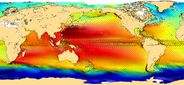
_ AVISO mean dynamic topography _
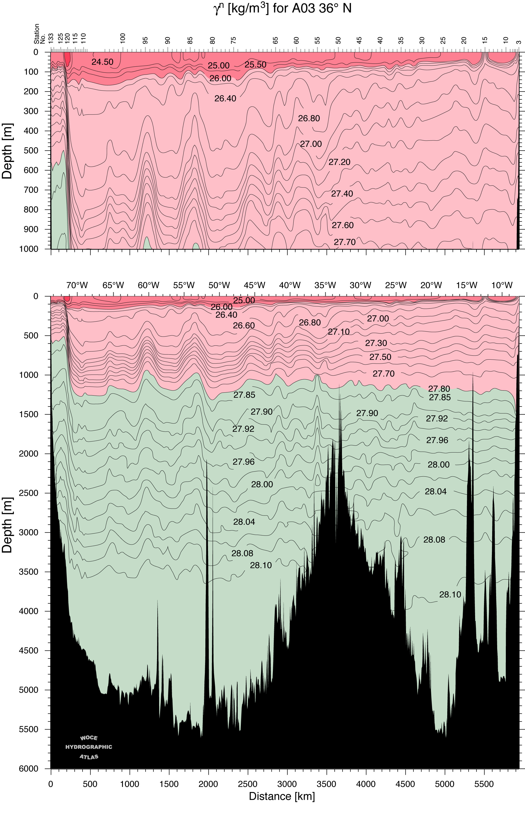
Thermal Wind
The geostrophic flow is determined by the pressure and the pressure is determined by the density (via hydrostatic balance). We can see this relationship more clearly if we take the derivative in \(z\) of the geostrophic equations:
These equations, called thermal wind relate the vertical shear of the geostrophic flow to the horizontal gradients of buoyancy. They are very useful for interpreting hydrographic data.
import pooch
import xarray as xr
from matplotlib import pyplot as plt

url = "ftp://ftp.spacecenter.dk/pub/DTU10/2_MIN/DTU10MDT_2min.nc"
fname = pooch.retrieve(url, known_hash="5d8eb0782514ca5f061eecc5a726f05b34a6ca34281cd644ad19c059ea8b528f")
ds = xr.open_dataset(fname)
ds
Downloading data from 'ftp://ftp.spacecenter.dk/pub/DTU10/2_MIN/DTU10MDT_2min.nc' to file '/home/jovyan/.cache/pooch/cd1481012b784d34e848db69c19b022f-DTU10MDT_2min.nc'.
SHA256 hash of downloaded file: 5d8eb0782514ca5f061eecc5a726f05b34a6ca34281cd644ad19c059ea8b528f
Use this value as the 'known_hash' argument of 'pooch.retrieve' to ensure that the file hasn't changed if it is downloaded again in the future.
<xarray.Dataset>
Dimensions:  (lon: 10801, lat: 5400)
Coordinates:
  * lon      (lon) float64 0.0 0.03333 0.06667 0.1 ... 359.9 359.9 360.0 360.0
  * lat      (lat) float64 -89.98 -89.95 -89.92 -89.88 ... 89.92 89.95 89.98
Data variables:
    mdt      (lat, lon) float32 ...
Attributes:
    Conventions:  COARDS/CF-1.0
    title:        DTU10MDT_2min.mdt.nc
    source:       Danish National Space Center
node_offset: 1- lon: 10801
- lat: 5400
- lon(lon)float640.0 0.03333 0.06667 ... 360.0 360.0
- long_name :
- longitude
- units :
- degrees_east
- actual_range :
- [-1.66666667e-02 3.60016667e+02]
array([0.000000e+00, 3.333333e-02, 6.666667e-02, ..., 3.599333e+02, 3.599667e+02, 3.600000e+02]) - lat(lat)float64-89.98 -89.95 ... 89.95 89.98
- long_name :
- latitude
- units :
- degrees_north
- actual_range :
- [-90. 90.]
array([-89.983333, -89.95    , -89.916667, ...,  89.916667,  89.95    ,
        89.983333])
- mdt(lat, lon)float32...
- long_name :
- mean ocean dynamic topography
- units :
- m
- actual_range :
- [-2.26 2.155]
[58325400 values with dtype=float32]
- Conventions :
- COARDS/CF-1.0
- title :
- DTU10MDT_2min.mdt.nc
- source :
- Danish National Space Center
- node_offset :
- 1
mdt = ds.mdt.coarsen(lon=10, lat=10, boundary='pad').mean()
import cartopy.crs as ccrs
proj = ccrs.Robinson(central_longitude=180)

fig = plt.figure(figsize=(16, 6))
ax = plt.axes(projection=proj, facecolor='0.8')
mdt.plot(ax=ax, transform=ccrs.PlateCarree())
ax.coastlines()
<cartopy.mpl.feature_artist.FeatureArtist at 0x7f424f265790>
